HIV 1 coreceptor usage prediction without multiple alignments: an application of string kernels

Open Access

Research

HIV-1 coreceptor usage prediction without multiple alignments: an

application of string kernels

Sébastien Boisvert

_{, Mario Marchand}

_{, François Laviolette}

_and

Jacques Corbeil*

Address: 1_{Centre de recherche du centre hospitalier de l'Université Laval, Québec (QC), Canada and} 2_{Département d'informatique et de génie} logiciel, Université Laval, Québec (QC), Canada

Email: Sébastien Boisvert - [email protected]; Mario Marchand - [email protected]; François Laviolette - [email protected]; Jacques Corbeil* - [email protected] * Corresponding author

Abstract

Background: Human immunodeficiency virus type 1 (HIV-1) infects cells by means of ligand-receptor interactions. This lentivirus uses the CD4 ligand-receptor in conjunction with a chemokine coreceptor, either CXCR4 or CCR5, to enter a target cell. HIV-1 is characterized by high sequence variability. Nonetheless, within this extensive variability, certain features must be conserved to define functions and phenotypes. The determination of coreceptor usage of HIV-1, from its protein envelope sequence, falls into a well-studied machine learning problem known as classification. The support vector machine (SVM), with string kernels, has proven to be very efficient for dealing with a wide class of classification problems ranging from text categorization to protein homology detection. In this paper, we investigate how the SVM can predict HIV-1 coreceptor usage when it is equipped with an appropriate string kernel.

Results: Three string kernels were compared. Accuracies of 96.35% (CCR5) 94.80% (CXCR4) and 95.15% (CCR5 and CXCR4) were achieved with the SVM equipped with the distant segments kernel on a test set of 1425 examples with a classifier built on a training set of 1425 examples. Our datasets are built with Los Alamos National Laboratory HIV Databases sequences. A web server is available at http://genome.ulaval.ca/hiv-dskernel.

Conclusion: We examined string kernels that have been used successfully for protein homology detection and propose a new one that we call the distant segments kernel. We also show how to extract the most relevant features for HIV-1 coreceptor usage. The SVM with the distant segments kernel is currently the best method described.

Background

The HIV-1 genome contains 9 genes. One of the genes, the

env gene, codes for 2 envelope proteins named gp41 and gp120. The gp120 envelope protein must bind to a CD4 receptor and a coreceptor prior to cell infection by HIV-1.

Two coreceptors can be used by HIV-1: the CCR5 (chem-okine receptor 5) and the CXCR4 (chem(chem-okine receptor 4). Some viruses are only capable of using the CCR5 corecep-tor. Other viruses can only use the CXCR4 corecepcorecep-tor. Finally, some HIV-1 viruses are capable of using both of Published: 4 December 2008

Retrovirology 2008, 5:110 doi:10.1186/1742-4690-5-110

Received: 14 July 2008 Accepted: 4 December 2008

This article is available from: http://www.retrovirology.com/content/5/1/110

© 2008 Boisvert et al; licensee BioMed Central Ltd.

these coreceptors. The pathology of a strain of HIV-1 is partly a function of the coreceptor usage [1]. The faster CD4+ cell depletion caused by CXCR4-using viruses [2] makes the accurate prediction of coreceptor usage medi-cally warranted. Specific regions of the HIV-1 external envelope protein, named hypervariable regions, contrib-ute to the turnover of variants from a phenotype to another [3]. HIV-1 tropisms (R5, X4, R5X4) are often (but not always) defined in the following way. R5 viruses are those that can use only the CCR5 coreceptor and X4 viruses are those that can use only the CXCR4 coreceptor. R5X4 viruses, called dual-tropic viruses, can use both core-ceptors. Tropism switch occurs during progression towards AIDS. Recently, it has been shown that R5 and X4 viruses modulate differentially host gene expression [4].

Computer-aided prediction

The simplest method used for HIV-1 coreceptor usage pre-diction is known as the charge rule [5,6]. It relies only on the charge of residues at positions 11 and 25 within the V3 loop aligned against a consensus. The V3 loop is the third highly variable loop in the retroviral envelope protein gp120. Nonetheless, other positions are also important since the removal of these positions gave predictors with comparable (but weaker) performance to those that were trained with these positions present [1]. Other studies [7-12] also outlined the importance of other positions and proposed machine learning algorithms, such as the ran-dom forest [11] and the support vector machine (SVM) with structural descriptors [10], to built better predictors (than the charge rule). Available predictors (through web-servers) of HIV-1 coreceptor usage are enumerated in [13].

An accuracy of 91.56% for the task of predicting the CXCR4 usage was obtained by [10]. Their method, based on structural descriptors of the V3 loop, employed a single dataset containing 432 sequences without indels and required the multiple alignment of all V3 sequences. However, such a prior alignment before learning might remove information present in the sequences which is rel-evant to the coreceptor usage task. Furthermore, a prior multiple alignment done on all the data invalidates the cross-validation method since the testing set in each fold has been used for the construction of the tested classifier. Another drawback of having an alignment-based method is that sequences having too many indels (when com-pared to a consensus sequence) are discarded to prevent the multiple alignment from yielding an unacceptable amount of gaps. In this paper, we present a method for predicting the coreceptor usage of HIV-1 which does not perform any multiple alignment prior to learning.

The SVM [14] has proven to be very effective at generating classifiers having good generalization (i.e., having high predicting accuracy). In particular, [1] have obtained a

sig-nificantly improved predictor (in comparison with the charge rule) with an SVM equipped with a linear kernel. However, the linear kernel is not suited for sequence clas-sification since it does not provide a natural measure of dissimilarity between sequences. Moreover, a SVM with a linear kernel can only use sequences that are exactly of the same length. Consequently, [1] aligned all HIV-1 V3 loop sequences with respect to a consensus. No such alignment was performed in our experiments. In contrast, string ker-nels [15] do not suffer from these deficiencies and have been explicitly designed to deal with strings and sequences of varying lengths. Furthermore, they have been successfully used for protein homology detection [16] – a classification problem which is closely related to the one treated in this paper.

Consequently, we have investigated the performance of the SVM, equipped with the appropriate string kernel, at predicting the coreceptor used by HIV-1 as a function of its protein envelope sequence (the V3 loop). We have compared two string kernels used for protein homology detection, namely the blended spectrum kernel [15,17] and the local alignment kernel [16], to a newly proposed string kernel, that we called the distant segments (DS) ker-nel.

Applications

Bioinformatic methods for predicting HIV phenotypes have been tested in different situations and the concord-ance is high [18-21].

As described in [18], current bioinformatics programs are underestimating the use of CXCR4 by dual-tropic viruses in the brain. In [19], a concordance rate of 91% was obtained between genotypic and phenotypic assays in a clinical setting of 103 patients. In [20], the authors showed that the SVM with a linear kernel achieves a con-cordance of 86.5% with the Trofile assay and a concord-ance of 79.7% with the TRT assay. Recombinant assays (Trofile and TRT) are described in [20].

Further improvements in available HIV classifiers could presumably allow the replacement of in vitro phenotypic assays by a combination of sequencing and machine learning to determine the coreceptor usage. DNA sequenc-ing is cheap, machine learnsequenc-ing technologies are very accu-rate whereas phenotypic assays are labor-intensive and take weeks to produce readouts [13]. Thus, the next gener-ation of bioinformatics programs for the prediction of coreceptor usage promises major improvements in clini-cal settings.

Methods

a discriminative learning algorithm used for binary classi-fication problems. For these problems, we are given a

training set of examples, where each example is labelled as being either positive or negative. In our case, each example is a string s of amino acids. When the binary classification task consists of predicting the usage of CCR5, the label of string s is +1 if s is the V3 loop of the protein envelope sequence of a HIV-1 virion that uses the CCR5 coreceptor, and -1 otherwise. The same method applies for the predic-tion of the CXCR4 coreceptor usage. When the binary clas-sification task consists of predicting the capability of utilizing CCR5 and CXCR4 coreceptors, the label of string

s is +1 if s is the V3 loop of the protein envelope sequence of a HIV-1 virion that uses both the CCR5 and CXCR4 coreceptors, and -1 if it is a virion that does not use CCR5 or does not use CXCR4.

Given a training set of binary labelled examples, each gen-erated according to a fixed (but unknown) distribution D, the task of the learning algorithm is to produce a classifier

f which will be as accurate as possible at predicting the correct class y of a test string s generated according to D

(i.e., the same distribution that generated the training set). More precisely, if f (s) denotes the output of classifier f on input string s, then the task of the learner is to find f that minimizes the probability of error . A

clas-sifier f achieving a low probability of error is said to gener-alize well (on examples that are not in the training set).

To achieve its task, the learning algorithm (or learner) does not have access to the unknown distribution D, but only to a limited set of training examples, each generated according to D. It is still unknown exactly what is best for the learner to optimize on the training set, but the learn-ing strategy used by the SVM currently provides the best empirical results for many practical binary classification tasks. Given a training set of labelled examples, the learn-ing strategy used by the SVM consists at findlearn-ing a soft-margin hyperplane [14,22], in a feature space of high dimensionality, that achieves the appropriate trade-off between the number of training errors and the magnitude of the separating margin realized on the training examples that are correctly classified (see, for example, [15]).

In our case, the SVM is used to classify strings of amino acids. The feature space, upon which the separating hyper-plane is built, is defined by a mapping from each possible string s to a high-dimensional vector ϕ(s). For example, in the case of the blended spectrum kernel [15], each compo-nent ϕα(s) is the frequency of occurrence in s of a specific substring αthat we call a segment. The whole vector ϕ(s) is the collection of all these frequencies for each possible

segment of at most p symbols. Consequently, vector ϕ(s) has components for an alphabet Σ containing

|Σ| symbols. If w denotes the normal vector of the separat-ing hyperplane, and b its bias (which is related to the dis-tance that the hyperplane has from the origin), then the output f (s) of the SVM classifier, on input string s, is given by

f (s) = sgn (冬w, ϕ(s)冭 + b),

where sgn(a) = +1 if a > 0 and -1 otherwise, and where 冬w,

ϕ(s)冭 denotes the inner product between vectors w and ϕ

(s). We have 冬w, ϕ (s)冭 = for d -dimensional vectors. The normal vector w is often called the discriminant or the weight vector.

Learning in spaces of large dimensionality

Constructing a separating hyperplane in spaces of very large dimensionality has potentially two serious draw-backs. The first drawback concerns the obvious danger of

overfitting. Indeed, with so many degrees of freedom for a vector w having more components than the number of training examples, there may exist many different w hav-ing a high probability of error while makhav-ing very few training errors. However, several theoretical results [15,22] indicate that overfitting is unlikely to occur when a large separating margin is found on the (numerous) cor-rectly classified examples – thus giving theoretical support to the learning strategy used by the SVM.

The second potential drawback concerns the computa-tional cost of using very high dimensional feature vectors

ϕ(s₁), ϕ (s₂),..., ϕ(s_m) of training examples. As we now demonstrate, this drawback can elegantly be avoided by using kernels instead of feature vectors. The basic idea con-sists of representing the discriminant w as a linear combi-nation of the feature vectors of the training examples. More precisely, given a training set {(s₁, y₁), (s₂, y₂),..., (s_m,

ym)} and a mapping ϕ(·), we write . The set {α₁,..., α_m} is called the dual representation of the (primal) weight vector w. Consequently, the inner prod-uct 冬w, ϕ(s)冭, used for computing the output of an SVM classifier, becomes

Pr ( ( ) ) ( , )~s y D f s ≠y

| |Σ i i p

=

∑

〈w s〉 =

∑

d

, ( )φ ₁ φ( )

w _{i i}y s_i

i m

=

∑

1

〈 〉 = 〈 〉 =

= =

∑

∑

w s _{i i}y s_i s y k s s

i m

i i i i

m

, ( )φ α φ( ), ( )φ α ( , ),

where defines the kernel function

asso-ciated with the feature map ϕ(·). With the dual represen-tation, the SVM classifier is entirely described in terms of the training examples s_i having a non-zero value for α_i. These examples are called support vectors. The so-called "kernel trick" consists of using k (s, t) without explicitly computing 冬ϕ(s), ϕ(t)冭 – a computationally prohibitive task for feature vectors of very large dimensionality. This is possible for many feature maps ϕ(·). Consider again, for example, the blended spectrum (BS) kernel where each component ϕα(s) is the frequency of occurrence of a seg-ment αin string s (for all words of at most p characters of an alphabet Σ). In this case, instead of performing

multiplications to compute explicitly 冬ϕ(s), ϕ (t)冭, we can compute, for each position i in string s and each position j in string t, the number of consecutive sym-bols that matches in s and t. We use the big-Oh notation to provide an upper bound to the running time of algo-rithms. Let T (n) denote the execution time of an algo-rithm on an input of size n. We say that T (n) is in O (g

(n)) if and only if there exists a constant c and a critical n₀

such that T (n) ≤cg (n) for all n ≥n₀. The blended spec-trum kernel requires at most O (p·|s|·|t|) time for each string pair (s, t) – an enormous improvement over the Ω (|Σ|p_{) time required for the explicit computation of the} inner product between a pair of feature vectors. In fact, there exists an algorithm [15] for computing the blended spectrum kernel in O (p·max (|s|, |t|)) time.

The distant segments kernel

The blended spectrum kernel is interesting because it con-tains all the information concerning the population of segments that are present in a string of symbols without considering their relative positions. Here, we propose the

distant segments (DS) kernel that, in some sense, extends the BS kernel to include (relative) positional information of segments in a string of symbols.

If one considers the frequencies of all possible segment distances inside a string as its features, then a precise com-parison can be done between any pair of strings. Remote protein homology can be detected using distances between polypeptide segments [23]. For any string s of amino acids, these authors used explicitly a feature vector

ϕ (s) where each component ϕ_{d, α, α'} (s) denotes the number of times the (polypeptide) segment α' is located at distance d (in units of symbols) following the (polypep-tide) segment α. They have restricted themselves to the

case where α and α' have the same length p, with p ≤ 3. Since the distance d is measured from the first symbol in

αto the first symbol in α', the d = 0 components of ϕ(s),

i.e., ϕ_0,α,α' (s), are non-zero only for α= α' and represent the number of occurrences of segment αin string s. Con-sequently, this feature vector strictly includes all the com-ponents of the feature vector associated with the BS kernel but is limited to segments of size p (for p ≤ 3). By working with the explicit feature vectors, these authors were able to obtain easily the components of the discriminant vector w

that are largest in magnitude and, consequently, are the most relevant for the binary classification task. However, the memory requirement of their algorithm increases exponentialy in p. Not surprisingly, only the results for p ≤

3 were reported by [23].

Despite these limitations, the results of [23] clearly show the relevance of having features representing the fre-quency of occurrences of pairs of segments that are sepa-rated by some distance for protein remote homology detection. Hence, we propose in this section the distance segments (DS) kernel that potentially includes all the fea-tures considered by [23] without limiting ourselves to p ≤

3 and to the case where the words (or segments) have to be of the same length. Indeed, we find no obvious biolog-ical motivation for these restrictions. Also, as we will show, there is no loss of interpretability of the results by using a kernel instead of the feature vectors. In particular, we can easily obtain the most significant components of the discriminant w by using a kernel. We will show that the time and space required for computing the kernel matrix and obtaining the most significant components of the discriminant w are bounded polynomially in terms of all the relevant parameters.

Consider a protein as a string of symbols from the alpha-bet Σ of amino acids. Σ* represents the set of all finite strings (including the empty string). For μ ∈ Σ*, |μ| denotes the length of the string μ. Throughout the paper,

s, t, α, μand νwill denote strings of Σ*, whereas θand δ will be lengths of such strings. Moreover, μνwill denote the concatenation of μand ν. The DS kernel is based on the following set. Given a string s, let be the set

of all the occurrences of substrings of length δ that are beginning by segment αand ending by segment α'. More precisely,

Note that the substring length δis related to the distance

d of [23] by δ= d + |α'| where d = |α| + |ν| when |α| and

k s t( , )def= 〈φ( ), ( )s φ t 〉

| |Σ i i p

=

∑

α αδ, ′( )s

δ_{α α},′( )s ={( , , ,μ α ν α μ′ ′, ) :s=μανα μ′ ′ ∧ ≤|α|∧ ≤ ′ ∧ ≤|α| | |ν ∧δ def

1 1 0 ==| | |s − μ| |− μ′|}.

|α'| do not overlap. Note also that, in contrast with [23], we may have |α| ≠ |α'|. Moreover, the segments αand α'

never overlap since μανα' μ' equals to the whole string s

and 0 ≤ |ν|. We have made this choice because it appeared biologically more plausible to have a distance ranging from the end of the first segment to the beginning of the second segment. Nevertheless, we will see shortly that we can include the possibility of overlap between segments with a very minor modification of the kernel.

The DS kernel is defined by the following inner product

where is the feature vector

Hence, the kernel is computed for a fixed maximum value

θ_m of segment sizes and a fixed maximum value δ_m of sub-string length. Note that, the number of sub-strings of size θof

Σ* grows exponentially with respect to θ. Fortunately, we are able to avoid this potentially devastating

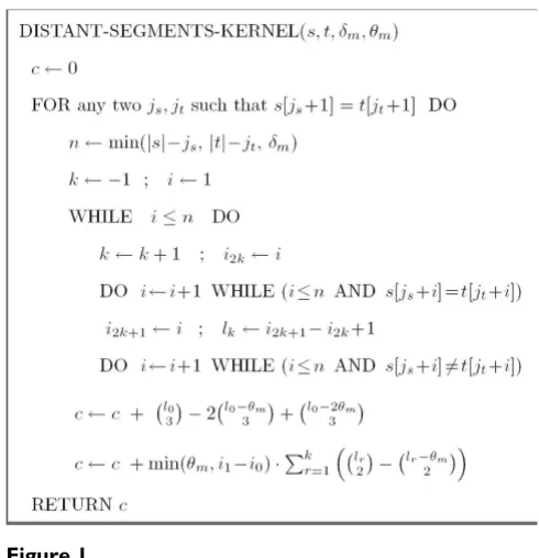
combinato-rial explosion in our computation of . Figure 1 shows the code of the algorithm. In the pseudo-code, s [i] denotes the symbol located at position i in the string s (with i ∈ {1, 2,..., |s|}). Moreover, for any integers

i, j, denotes if 0 ≤ i ≤ j, and 0 otherwise.

Admittedly, it is certainly not clear that the algorithm of

Figure 1 actually computes the value of given

by Equation 2. Hence, a proof of correctness of this algo-rithm is presented at the appendix (located after the con-clusion). The worst-case running time is easy to obtain because the algorithm is essentially composed of three imbricated loops: one for j_s ∈ {0,..., |s|-1}, one for j_t ∈

{0,..., |t|-1}, and one for i ∈ {1,..., min(|s|, |t|, δ_m)}. The time complexity is therefore in O (|s|·|t|·min(|s|, |t|,

δ_m)).

Note that the definition of the DS-kernel can be easily modified in order to accept overlaps between α and α'. Indeed, when overlaps are permitted, they can only occur when both αand α' start and end in {j_s + i₀,..., j_s + i₁-1}. The number of elements of for which i2r ≤δ<i2r+1 is thus the same for all values of r, including r = 0.

Conse-quently, the algorithm to compute the DS kernel, when overlaps are permitted, is the same as the one in Figure 1 except that we need the replace the last two lines of the FOR loop, involved in the computation of c, by the single line:

Similar simple modifications can be performed for the more restrictive case of |α| = |α'|.

Extracting the discriminant vector with the distant segments kernel

We now show how to extract (with reasonable time and space resources) the components of the discriminant w

that are non-zero. Recall that when the

SVM contains l support vectors {(s₁, y₁),..., (s_l, y_l)}. Recall

also that each feature ϕδ, α, α' (si) is identified by a triplet (δ,

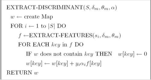
α, α'), with δ≥ |α| + |α'|. Hence, to obtain the non-zero valued components of w, we first obtain the non-zero val-ued features ϕ_{δ, α, α'} (s_i) from each support vector (with Algorithm EXTRACT-FEATURES of Figure 2) and then col-lect and merge every feature of each support vector by multiplying each of them by αiyi (with Algorithm EXTRACT-DISCRIMINANT of Figure 3).

k_DSδ θm,m_{( , )}s t = 〈φ_DSδ θm, m_{( ),}s φ_DSδ θm, m_{( ) ,}t 〉 def

(2)

φ_DSδ θm,m_{( )s}

φδ θ

α α δ

δ α α α θ α θ α

DSm m

m m

s s

,

,

{( , , ): | | | | | | ( ) =

(

)

′ ≤ ≤ ∧ ≤ ′ ≤ ∧

def



1 1 ++ ′ ≤ ≤| |α δ δm}.

k_DSδ θm, m_{( , )}s t

j i ⎛ ⎝ ⎜ ⎞

⎠

⎟ _{i!(j i}j₋! _)!

k_DSδ θm,m_{( , )}s t

_{( , )j j}

s t

c c _m i i lr lr m

r k

← + − ⋅ ⎛

⎝

⎜ ⎞

⎠

⎟ −⎛ −

⎝

⎜ ⎞

⎠ ⎟ ⎛

⎝

⎜⎜ ⎞_⎠⎟⎟

=

∑

min(θ , _{1 0}) θ .

0 2 2

w _i i iy si l

=

∑

The algorithm for computing

Figure 1

We transform each support vector ϕ(s_i) into a Map of fea-tures. Each Map key is an identifier for a (δ, α, α') having

ϕδ, α, α' (si) > 0. The Map value is given by ϕδ, α, α'(si) for each key.

The worst-case access time for an AVL-tree-Map of n ele-ments is O (log n). Hence, from Figure 2, the time com-plexity of extracting all the (non-zero valued) features of a

support vector is in .

Moreo-ver, since the total number of features inserted to the Map by the algorithm EXTRACT-DISCRIMINANT is at most

, the time complexity of extracting all the

non-zero valued components of w is in

.

SVM

We have used a publicly available SVM software, named SVMlight _{[24], for predicting the coreceptor usage. Learning} SVM classifier requires to choose the right trade-off between training accuracy and the magnitude of the sepa-rating margin on the correctly classified examples. This trade-off is generally captured by a so-called soft-margin hyperparameter C.

The learner must choose the value of C from the training set only – the testing set must be used only for estimating the performance of the final classifier. We have used the (well-known) 10-fold cross-validation method (on the training set) to determine the best value of C and the best values of the kernel hyperparameters (that we describe below). Once the values of all the hyperparameters were found, we used these values to train the final SVM classi-fier on the whole training set.

Selected metrics

The testing of the final SVM classifier was done according to several metrics. Let P and N denote, respectively, the number of positive examples and the number of negative examples in the test set. Let TP, the number of "true posi-tives", denote the number of positive testing examples that are classified (by the SVM) as positive. A similar defi-nition applies to TN, the number of "true negatives". Let FP, the number of "false positives", denote the number of negative testing examples that are classified as positive. A similar definition applied to FN, the number of "false neg-atives". To quantify the "fitness" of the final SVM classi-fier, we have computed the accuracy, which is (TP+TN)/ (P+T), the sensitivity, which is TP/P, and the specificity, which is TN/N. Finally, for those who cannot decide how much to weight the cost of a false positive, in comparison

O s(| |θ δ_{m m}2 ⋅log(| |s θ δ_{m m}2 ))

l s⋅| |⋅θ δ_{m m}2

O l s( | |θ δ_{m m}2 ⋅log( | |l s θ δ_{m m}2 ))

The algorithm for extracting the features of a string s into a Map

Figure 2

with a false negative, we have computed the "area under the ROC curve" as described by [25].

Unlike the other metrics, the accuracy (which is 1 – the testing error) has the advantage of having very tight confi-dence intervals that can be computed straightforwardly from the binomial tail inversion, as described by [26]. We have used this method to find if whether or not the observed difference of testing accuracy (between two clas-sifiers) was statistically significant. We have reported the results only when a statistically significant difference was observed with a 90% confidence level.

Selected string kernels

One of the kernel used was the blended spectrum (BS) kernel that we have described above. Recall that the fea-ture space, for this kernel, is the count of all k-mers with 1

≤k ≤p. Hence p is the sole hyperparameter of this kernel.

We have also used the local alignment (LA) kernel [16] which can be thought of as a soft-max version of the Smith-Waterman local alignment algorithm for pair of sequences. Indeed, instead of considering the alignment that maximizes the Smith-Waterman (SW) score, the LA kernel considers every local alignment with a Gibbs distri-bution that depends on its SW score. Unfortunately, the LA kernel has too many hyperparameters precluding their

optimization by cross-validation. Hence, a number of choices were made based on the results of [16]. Namely, the alignment parameters were set to (BLOSUM 62, e = 11, d = 1) and the empirical kernel map of the LA kernel was used. The hyperparameter βwas the only one that was adjusted by cross-validation.

Of course, the proposed distant segments (DS) kernel was also tested. The θ_m hyperparameter was set to δ_m to avoid the limitation of segment length. Hence, δ_m was the sole hyperparameter for this kernel that was optimized by cross-validation.

Other interesting kernels, not considered here because they yielded inferior results (according to [16], and [23]) on the remote protein homology detection problem, include the mismatch kernel [27] and the pairwise kernel [28].

Datasets

The V3 loop sequence and coreceptor usage of HIV-1 sam-ples were retrieved from Los Alamos National Laboratory HIV Databases http://www.hiv.lanl.gov/ through availa-ble online forms.

Every sample had a unique GENBANK identifier. Sequences containing #, $ or * were eliminated from the

The algorithm for merging every feature from the set S = {(s₁, y₁), (s₂, y₂),

Figure 3

dataset. The signification of these symbols was reported by Brian Foley of Los Alamos National Laboratory (per-sonal communication). The # character indicates that the codon could not be translated, either because it had a gap character in it (a frame-shifting deletion in the virus RNA), or an ambiguity code (such as R for purine). The $ and * symbols represent a stop codon in the RNA sequence. TAA, TGA or TAG are stop codons. The dataset was first shuffled and then splitted half-half, yielding a training and a testing set. The decision to shuffle the dataset was made to increase the probability that both the training and testing examples are obtained from the same distribu-tion. The decision to use half of the dataset for testing was made in order to obtain tight confidence intervals for accuracy.

Samples having the same V3 loop sequence and a differ-ent coreceptor usage label are called contradictions. Contra-dictions were kept in the datasets to have prediction performances that take into account the biological reality of dual tropism for which frontiers are not well defined.

Statistics were compiled for the coreceptor usage distribu-tion, the count of contradictions, the amount of samples in each clades and the distribution of the V3 loop length.

Results

Here we report statistics on our datasets, namely the dis-tribution, contradictions, subtypes and the varying lengths. We also show the results of our classifiers on the HIV-1 coreceptor usage prediction task, a brief summary of existing methods and an analysis of the discriminant vector with the distant segments kernel.

Statistics

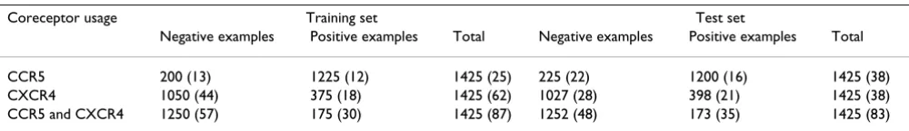
In Table 1 is reported the distribution of coreceptor usages in the datasets created from Los Alamos National Labora-tory HIV Databases data. In the training set, there are 1225 CCR5-utilizing samples (85.9%), 375 CXCR4-utilizing samples (26.3%) and 175 CCR5-and-CXCR4-utilizing samples (12.2%). The distribution is approximatly the same in the test set. There are contradictions (entries with the same V3 sequence and a different coreceptor usage) in all classes of our datasets. A majority of viruses can use CCR5 in our datasets.

In Table 2, the count is reported regarding HIV-1 subtypes, also known as genetic clades. HIV-1 subtype B is the most numerous in our datasets. The clade information is not an attribute that we provided to our classifiers, we only built our method on the primary structure of the V3 loop. Therefore, our method is independant of the clades.

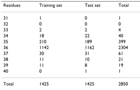
The V3 loops have variable lengths among the virions of a population. In our dataset (Table 3), the majority of sequences has exactly 36 residues, although the length ranges from 31 to 40.

Coreceptor usage predictions

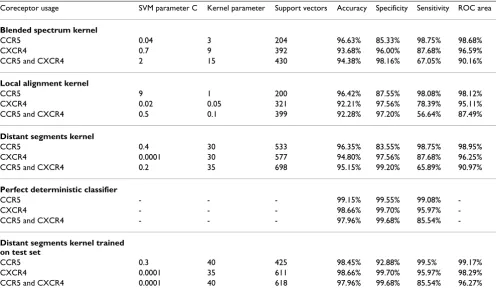
Classification results on the three different tasks (CCR5, CXCR4, CCR5-and-CXCR4) are presented in Table 4 for three different kernels.

For the CCR5-usage prediction task, the SVM classifier achieved a testing accuracy of 96.63%, 96.42%, and 96.35%, respectively, for the BS, LA, and DS kernels. By using the binomial tail inversion method of [26], we find no statistically significant difference, with 90% confi-dence, between kernels.

For the CXCR4-usage prediction task, the SVM classifier achieved a testing accuracy of 93.68%, 92.21%, and 94.80%, respectively, for the BS, LA, and DS kernels. By using the binomial tail inversion method of [26], we find that the difference is statistically significant, with 90% confidence, for the DS versus the LA kernel.

For the CCR5-and-CXCR4-usage task, the SVM classifier achieved a testing accuracy of 94.38%, 92.28 %, and 95.15%, respectively, for the BS, LA, and DS kernels. Again, we find that the difference is statistically signifi-cant, with 90% confidence, for the DS versus the LA ker-nel.

Overall, all the tested string kernels perform well on the CCR5 task, but the DS kernel is significantly better than the LA kernel (with 90% confidence) for the CXCR4 and CCR5-and-CXCR4 tasks. For these two prediction tasks, the performance of the BS kernel was closer to the one obtained for the DS kernel than the one obtained for the LA kernel.

Table 1: Datasets. Contradictions are in parenthesis.

Coreceptor usage Training set Test set

Negative examples Positive examples Total Negative examples Positive examples Total

CCR5 200 (13) 1225 (12) 1425 (25) 225 (22) 1200 (16) 1425 (38)

CXCR4 1050 (44) 375 (18) 1425 (62) 1027 (28) 398 (21) 1425 (38)

Classification with the perfect deterministic classifier Also present in Table 4 are the results of the perfect deter-ministic classifier. This classifier is the deterministic classi-fier achieving the highest possible accuracy on the test set. For any input string s in a testing set T, the perfect deter-minist classifier (h*) returns the most frequently encoun-tered class label for string s in T. Hence, the accuracy on T

of h* is an overall measure of the amount of contradic-tions that are present in T. There are no contradictions in

T if and only if the testing accuracy of h* is 100%. As shown in Table 4, there is a significant amount of contra-dictions in the test set T. These results indicate that any deterministic classifier cannot achieve an accuracy greater than 99.15%, 98.66% and 97.96%, respectively for the CCR5, CXCR4, and CCR5-and-CXCR4 coreceptor usage tasks.

Discriminative power

To determine if a SVM classifier equipped with the distant segments (DS) kernel had enough discriminative power to achieve the accuracy of perfect determinist classifier, we trained the SVM, equipped with the DS kernel, on the test-ing set. From the results of Table 4, we conclude that the SVM equipped with the DS kernel possess sufficient dis-criminative power since it achieved (almost) the same accuracy as the perfect deterministic classifier for all three tasks. Hence, the fact that the SVM with the DS kernel does not achieve the same accuracy as the perfect deter-minist classifier when it is obtained from the training set (as indicated in Table 4) is not due to a lack of discrimina-tive power from the part of the learner.

Discriminant vectors

The discriminant vector that maximizes the soft-margin has (almost always) many non-zero valued components which can be extracted by the algorithm of Figure 3. We examine which components of the discriminant vector have the largest absolute magnitude. These components

give weight to the most relevant features for a given classi-fication task. In Figure 4, we describe the most relevant features for each tasks. Only the 20 most significant fea-tures are shown.

A subset of positive-weighted features shown for CCR5-utilizing viruses are also in the negative-weighted features shown for CXCR4-utilizing viruses. Furthermore, a subset of positive-weighted features shown for CXCR4-utilizing viruses are also in the negative-weighted features reported for CCR5-utilizing viruses. Thus, CCR5 and CXCR4 discri-minant models are complementary. However, since 3 tro-pisms exist (R5, X4 and R5X4), features contributing to CCR5-and-CXCR4 should also include some of the fea-tures contributing to CCR5 and some of the feafea-tures con-tributing to CXCR4. Among shown positive-weighted features for CCR5-and-CXCR4, there are features that also contribute to CXCR4 ([8, R, R], [13, R, T], [9, R, R]). On another hand, this is not the case for CCR5. However, only the twenty most relevant features have been shown and there are many more features, with similar weights, that contribute to the discriminant vector. In fact, the clas-sifiers that we have obtained depend on a very large number of features (instead of a very small subset of rele-vant features).

Discussion

The proposed HIV-1 coreceptor-usage prediction tool achieved very high accuracy in comparison with other existing prediction methods. In view of the results of Pillai et al, we have shown that the SVM classification accuracy can be greatly improved with the usage of a string kernel. Surprisingly, the local alignment (LA) kernel, which makes an explicit use of biologically-motivated scoring matrices (such as BLOSUM 62), turns out to be outper-formed by the blended spectrum (BS) and the distant seg-ments (DS) kernels which do not try to exploit any concept of similarity between residues but rely, instead, on a very large set of easily-interpretable features. Thus, a Table 2: HIV-1 subtypes.

Subtype Training set Test set Total

A 39 46 85

B 955 943 1898

C 168 149 317

02_AG 12 15 27

O 11 11 22

D 69 95 164

A1 25 18 43

AG 5 5 10

01_AE 97 106 203

G 7 7 14

Others 37 30 67

Total 1425 1425 2850

Table 3: Sequence length distribution. The minimum length is 31 residues and the maximum length is 40 residues.

Residues Training set Test set Total

31 1 0 1

32 0 0 0

33 2 2 4

34 18 22 40

35 210 189 399

36 1142 1162 2304

37 30 31 61

38 11 10 21

39 11 8 19

40 0 1 1

weighted-majority vote over a very high number of simple features constitutes a very productive approach, that is both sensitive and specific to what it is trained for, and applies well in the field of viral phenotype prediction.

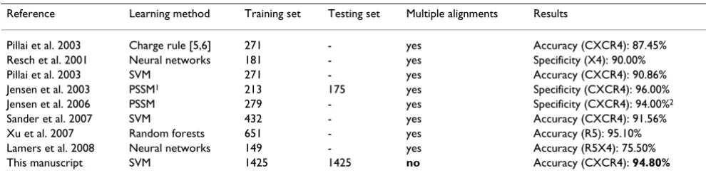
Comparison with available bioinformatic methods In Table 5, we show a summary of the available methods. The simplest method (the charge rule) has an accuracy of 87.45%. Thus, the charge rule is the worst method pre-sented in table 5. The SVM with string kernels is the only approach without multiple alignments. Therefore, V3 sequences with many indels can be used with our method, but not with the other. These other methods were not directly tested here with our datasets because they all rely on multiple alignments. The purpose of those alignments is to produce a consensus and to yield transformed sequences having all the same length. As indicated by the size of the training set in those methods, sequences having larger indels were discarded, thus making these datasets smaller. Most of the methods rely on cross-validation to perform quality assessment but, as we have mentioned, this is problematic when multiple alignments are per-formed prior to learning, since, in these cases, the testing set in each fold is used for the construction of the tested classifier. It is also important to mention that the various methods presented in Table 5 do not produce predictors

for the same coreceptor usage task. Indeed, the definition of X4 viruses is not always the same: some authors refer to it as CXCR4-only while other use it as CXCR4-utilizing. It is thus unfeasible to assess the fitness of these approaches, which are twisted by cross-validation, multiple align-ments and heterogeneous dataset composition.

The work by Lamers and colleagues [12] is the first devel-opment in HIV-1 coreceptor usage prediction regarding dual-tropic viruses. Using evolved neural networks, an accuracy of 75.50% was achieved on a training set of 149 sequences with the cross-validation method. However, the SVM equipped with the distant segments kernel reached an accuracy of 95.15% on a large test set (1425 sequences) in our experiments. Thus, our SVM outper-forms the neural network described by Lamers and col-leagues [12] for the prediction of dual-tropic viruses.

Los Alamos National Laboratory HIV Databases

Although we used only the Los Alamos National Labora-tory HIV Databases as our source of sequence informa-tion, it is notable that this data provider represents a meta-resource, fetching bioinformation from databases around the planet, namely GenBank (USA, http:// www.ncbi.nlm.nih.gov/Genbank/), EMBL (Europe, http:/ /www.ebi.ac.uk/embl/) and DDBJ (Japan, http:// Table 4: Classification results on the test sets. Accuracy, specificity and sensitivity are defined in Methods. See [25] for a description of the ROC area.

Coreceptor usage SVM parameter C Kernel parameter Support vectors Accuracy Specificity Sensitivity ROC area

Blended spectrum kernel

CCR5 0.04 3 204 96.63% 85.33% 98.75% 98.68%

CXCR4 0.7 9 392 93.68% 96.00% 87.68% 96.59%

CCR5 and CXCR4 2 15 430 94.38% 98.16% 67.05% 90.16%

Local alignment kernel

CCR5 9 1 200 96.42% 87.55% 98.08% 98.12%

CXCR4 0.02 0.05 321 92.21% 97.56% 78.39% 95.11%

CCR5 and CXCR4 0.5 0.1 399 92.28% 97.20% 56.64% 87.49%

Distant segments kernel

CCR5 0.4 30 533 96.35% 83.55% 98.75% 98.95%

CXCR4 0.0001 30 577 94.80% 97.56% 87.68% 96.25%

CCR5 and CXCR4 0.2 35 698 95.15% 99.20% 65.89% 90.97%

Perfect deterministic classifier

CCR5 - - - 99.15% 99.55% 99.08%

-CXCR4 - - - 98.66% 99.70% 95.97%

-CCR5 and CXCR4 - - - 97.96% 99.68% 85.54%

-Distant segments kernel trained on test set

CCR5 0.3 40 425 98.45% 92.88% 99.5% 99.17%

CXCR4 0.0001 35 611 98.66% 99.70% 95.97% 98.29%

www.ddbj.nig.ac.jp/). Researchers cannot directly send their HIV sequences to LANL, but it is clear that this approach makes this database less likely to contain errors.

Noise

The primary cause of contradictions (e.g. a sequence hav-ing two or more phenotypes) remains uncharacterized. It may be due to a particular mix, to some extent, of virion envelope attributes (regions other than the V3) and of the host cell receptor counterparts. As genotypic assays, based on bioinformatics prediction software, rely on sequencing technologies, they are likely to play a more important role in clinical settings as sequencing cost drops. Next-genera-tion sequencing platforms promise a radical improve-ment on the throughput and more affordable prices. Meanwhile, effective algorithmic methods with proven statistical significance must be developed. Bioinformatics practitioners have to innovate by creating new algorithms to deal with large datasets and need to take into consider-ation sequencing errors and noise in phenotypic assay rea-douts. Consequently, we investigated the use of statistical machine learning algorithms, such as the SVM, whose robustness against noise has been observed in many clas-sification tasks. The high accuracy results we have obtained here indicate that this is also the case for the task of predicting the coreceptor usage of HIV-1. While it remains uncertain whether or not other components of the HIV-1 envelope contribute to the predictability of the viral phenotype, we have shown that the V3 loop alone produces very acceptable outputs despite the presence of a small amount of noise.

Web server

To allow HIV researchers to test our method on the web, we have implemented a web server for the HIV-1 corecep-tor usage prediction. The address of this web server is http://genome.ulaval.ca/hiv-dskernel. In this setting, one has to submit fasta-formatted V3 sequences in a web form. Then, using the dual representation of the SVM with the distant segments kernel, the software predicts the corecep-tor usage of each submitted viral sequence. Those predic-tions are characterized by high accuracy (according to results in Table 4). Source codes for the web server and for a command-line back-end are available in additional file 1.

Conclusion

To our knowledge, this is the first paper that investigates the use of string kernels for predicting the coreceptor usage of HIV-1. Our contributions include a novel string kernel (the distant segments kernel), a SVM predictor for HIV-1 coreceptor usage with the identification of the most relevant features and state-of-the-art results on accuracy, specificity, sensitivity and receiver operating characteris-tic. As suggested, string kernels outperform all published Features (20 are shown) with highest and lowest weights for

each coreceptor usage prediction task

Figure 4

Features (20 are shown) with highest and lowest weights for each coreceptor usage prediction task.

7,R,G 8,R,Q 10,T,R 11,R,Y3,R,Y 5,R,G 20,R,I 6,R,I 9,R,R 14,R,G 10,N,P 11,NNT,P 11,NN,P 6,NT,I 10,T,G 22,NN,I 10,NT,P 2,N,N 21,N,I 5,T,I

A) CCR5 most relevant features

Weight

−6e−04 −4e−04 −2e−04 0e+00 2e−04 4e−04 6e−04

21,N,I 10,NT,P 17,NT,T 10,N,P 5,NT,S 5,N,S 11,NN,P 4,T,S 13,SI,T 12,C,SI8,P,R 18,R,G 13,R,T 11,R,Y 7,R,G 20,R,I 9,R,R 8,R,R 5,R,G 10,T,R

B) CXCR4 most relevant features

Weight

−5e−04 0e+00 5e−04

6,S,P 6,S,GP 7,S,PG 13,S,T 7,S,GPG 23,T,TG 24,CT,TG 14,SI,G 14,SI,TG 23,TR,TG4,R,H 21,R,IGDIR 7,G,H 2,R,I 9,R,R 5,N,R 20,R,IGDI 13,R,T 17,R,I 8,R,R

C) CCR5 and CXCR4 most relevant features

Weight

algorithms for HIV-1 coreceptor usage prediction. Large margin classifiers and string kernels promise improve-ments in drug selection, namely CCR5 coreceptor inhibi-tors and CXCR4 coreceptor inhibiinhibi-tors, in clinical settings. Since the binding of an envelope protein to a receptor/ coreceptor prior to infection is not specific to HIV-1, one could extend this work to other diseases. Furthermore, most ligand interactions could be analyzed in such a fash-ion. Detailed features in primary structures (DNA or pro-tein sequences) can be elucidated with the proposed bioinformatic method. Although we have exposed that even the perfect algorithm (entitled "Perfect determinist classifier") can not reach faultless outcomes, we have also empirically demonstrated that our algorithms are very competitive (more than 96% with distant segments for CCR5). It is thus feasible to apply kernel methods based on features in primary structures to compare sequence information in the perspective of predicting a phenotype. The distant segments kernel has broad applicability in HIV research such as drug resistance, coreceptor usage (as shown in this paper), immune escape, and other viral phenotypes.

Appendix

Proof of the correctness of the distant segments kernel We now prove that the algorithm

DISTANT-SEGMENTS-KERNEL (s, t, δ_m, θ_m) does, indeed, compute as defined by Equation 2.

Proof. For each pair (js, jt) such that s [js + 1] = t [jt + 1] and

each δ≥ 2, let us define to be the set of all triples (δ, (μ_s, α, ν_s, α', ), (μ_t, α, ν_t, α', )) such that

Clearly, is the sum of all the values of

| | over all the possible pairs (j_s, j_t). Moreover, it is

easy to see that | | can be computed only from the

knowledge of the set of indices i ∈ {1,..., n} satisfying property P (i) : = s [j_s + i] = t [j_t + i]. Note that when the test of the first WHILE loop is performed, the value of i is such that P (i) is valid but not P (i - 1). Moreover, in the second WHILE loop, P (i) remains valid, except for the last test. Thus, s [js + i] = t [jt + i] if and only if i2r ≤i <i2r+1 for some r ∈ {0,..., k}. This, in turn, implies that each element of must be such that i_2r ≤ δ <i_2r+1 for some r. To obtain the result, it is therefore sufficient to prove that both of theses properties hold.

P1 The number of elements of , for which i₀ <δ<i₁, is given by

P2 For r ∈ {1,..., k}, the number of elements of ,

for which i_2r ≤δ<i_2r+1, is given by

To prove these properties, we will use the fact that, if 1 ≤i

≤k, then counts the number of sequences 冬a₁,..., a_i冭

satisfying 1 ≤a₁ <a₂ < 傼 <a_i ≤k where {a₁, a₂, ..., a_i} are i

string positions. Moreover, for any substring u of s, let us denote by b_u the starting position of u in s, and by e_u the

k_DSδ θm,m_{( , )}s t

( , )j js t

′

μ_s μ′_t

− ≤

− ≤ ′ ≤

− ′ ′ ∈ ′

δ δ

α θ α θ

μ α ν α μ _{α α}δ m

m m

u u u u u

;

| | | | ;

( , , , , ) , ( )

and

for

 == =

− = =

s u t

j j

s s t t

and for and

;

|μ | |μ | .

k_DSδ θm,m_{( , )}s t

_{( , )j js t}

_{( , )j j}

s t

_{( , )j j}

s t

( , )j js t

l0 l0 m l0 m

3 2 3

2 3

⎛ ⎝

⎜ ⎞

⎠

⎟ − ⎛ −

⎝

⎜ ⎞

⎠

⎟ +⎛ −

⎝

⎜ ⎞

⎠ ⎟

θ θ

.

_{( , )j j}

s t

min(θ_m,i₁ i₀) lr l0 θm .

2 2

− ⋅ ⎛

⎝

⎜ ⎞

⎠

⎟ −⎛ −

⎝

⎜ ⎞

⎠ ⎟ ⎛

⎝

⎜⎜ ⎞_⎠⎟⎟

k i ⎛ ⎝ ⎜ ⎞

⎠ ⎟

Table 5: Available methods. The results column contains the metric and what the classifier is predicting.

Reference Learning method Training set Testing set Multiple alignments Results

Pillai et al. 2003 Charge rule [5,6] 271 - yes Accuracy (CXCR4): 87.45%

Resch et al. 2001 Neural networks 181 - yes Specificity (X4): 90.00%

Pillai et al. 2003 SVM 271 - yes Accuracy (CXCR4): 90.86%

Jensen et al. 2003 PSSM1 _{213 175 yes Specificity (CXCR4): 96.00%}

Jensen et al. 2006 PSSM 279 - yes Specificity (CXCR4): 94.00%2

Sander et al. 2007 SVM 432 - yes Accuracy (CXCR4): 91.56%

Xu et al. 2007 Random forests 651 - yes Accuracy (R5): 95.10%

Lamers et al. 2008 Neural networks 149 - yes Accuracy (R5X4): 75.50%

This manuscript SVM 1425 1425 no Accuracy (CXCR4): 94.80%

first position of s after the substring u (if s ends with u, choose e_u = |s| + 1).

We first prove P2. Fix an r. Since i₀ = 1, we have that any s -substring α of length ≤θ_m with bα= js + i0 and eα≤js + i1 together with any s-substring α' of length ≤θm such that

j_s + i_2r ≤bα' <eα' ≤js + i2r+1,

will give rise to exactly one element of with i_2r ≤δ

<i_2r+1. Conversely, each element such that i_2r ≤δ

<i_2r+1 will have an αand an α' with these properties. Since

αhas to start at j_s + i₀, it is easy to see that the number of such possible αis exactly min(θ_m, i₁ - i₀). Thus let us show

that the number of possible α' is exactly .

Since l_r gives the number of positions from j_s + i_2r to j_s +

i2r+1 inclusively, counts all the possible, choices of bα'

and eα' with js + i2r ≤bα' <eα' ≤js + i2r+1. Thus counts the

number of possible strings α' of all possible lengths (including lengths > θ_m). On another hand, the number of

α' having a length > θ_m. is equal to . Indeed, if l_r

-θm < 2, = 0 as wanted, and otherwise, there is a

one-to-one correspondence between the set of all sequences 冬a₁, a2冭 such that 1 ≤a₁ <a₂ ≤l_r - θ_m and the set of all α' of length > θ_m. The correspondence is obtained by putting b_α' = i_2r + a₁ - 1 and e_α' = i_2r + θ_m + a₂ - 1.

The proof for P1 is similar to the one for P2 except that we have to consider the fact that both αand α' start and end in {j_s + i₀,..., j_s + i₁ - 1}. Since no overlap is allowed and b_α

= j_s + i₀, we must have

j_s + i₀ ≤eα- 1 <bα' <eα' ≤js + i1.

Since l0 gives the number of positions from js + i0 to js + i1

inclusively, counts all the possible choices of αand

α' for all possible lengths. Recall that if l₀ < 3, which can

only occur if i₁ = i₀ + 1, we have that , as wanted.

On another hand, counts all the possible

choices of α of length > θ_m and of α' of arbitrary length. This set of possible choices is non empty only if l₀ - θ_m ≥ 3 and, then, the one-to-one correspondence between a sequence 冬a₁, a₂, a₃冭 such that 1 ≤a₁ <a₂ <a₃ ≤l₀ - θ_m and the values of 冬e_α, b_α', e_α'冭 is

eα- 1 = js + θm + a1, bα' = js + θm + a2 and eα' = js + θm + a3.

Similarly, counts all the possible choices of α' of

length > θ_m and of αof arbitrary length, the correspond-ence being eα- 1 = js + a1, bα' = js + a2 and eα' = js + θm + a3.

Finally, counts all the possible choices of αand

α', both of length > θ_m. In the cases where such possible choices exist (i.e., if l₀ - 2θ_m ≥ 3), the correspondence is eα - 1 = j_s + θ_m + a₁, bα' = js + θm + a2 and eα' = js + 2θm + a3. Then, property P1 immediately follows from the inclusion-exclusion argument.

Competing interests

The authors declare that they have no competing interests.

Authors' contributions

SB, MM, FL and JC drafted the manuscript. FL wrote the proof for the distant segments kernel. SB performed exper-iments. SB, MM, FL and JC approved the manuscript.

Additional material

Acknowledgements

This project was funded by the Canadian Institutes of Health Research and by the Natural Sciences and Engineering Research Council of Canada (MM, 122405 and FL, 262067). JC is the holder of Canada Research Chair in Med-ical Genomics.

References

1. Pillai S, Good B, Richman D, Corbeil J: A new perspective on V3 phenotype prediction. AIDS Res Hum Retroviruses 2003,

19:145-149. _{( , )j j}

s t

( , )j js t

lr lr m

2 2 ⎛ ⎝ ⎜ ⎞ ⎠ ⎟ −⎛ − ⎝ ⎜ ⎞ ⎠ ⎟ θ lr 2 ⎛ ⎝ ⎜ ⎞ ⎠ ⎟ lr 2 ⎛ ⎝ ⎜ ⎞ ⎠ ⎟

lr− m ⎛ ⎝ ⎜ ⎞ ⎠ ⎟ θ 2

lr− m ⎛ ⎝ ⎜ ⎞ ⎠ ⎟ θ 2 l₀ 3 ⎛ ⎝ ⎜ ⎞ ⎠ ⎟ l₀ 3 ⎛ ⎝ ⎜ ⎞ ⎠ ⎟

Additional file 1

Source code and data. Web server, classifiers, discriminant vectors and data sets.

Click here for file

[http://www.biomedcentral.com/content/supplementary/1742-4690-5-110-S1.zip]

l_{0 m}

3 − ⎛ ⎝ ⎜ ⎞ ⎠ ⎟ θ

l_{0 m}

3 − ⎛ ⎝ ⎜ ⎞ ⎠ ⎟ θ

l_{0 2 m}

Publish with BioMed Central and every scientist can read your work free of charge "BioMed Central will be the most significant development for disseminating the results of biomedical researc h in our lifetime."

Sir Paul Nurse, Cancer Research UK

Your research papers will be:

available free of charge to the entire biomedical community peer reviewed and published immediately upon acceptance cited in PubMed and archived on PubMed Central yours — you keep the copyright

Submit your manuscript here:

http://www.biomedcentral.com/info/publishing_adv.asp

BioMedcentral

2. Richman D, Bozzette S: The impact of the syncytium-inducing phenotype of human immunodeficiency virus on disease pro-gression. J Infect Dis 1994, 169:968-974.

3. Zhang L, Robertson P, Holmes EC, Cleland A, Leigh Brown A, Sim-monds P: Selection for specific V3 sequences on transmission of human immunodeficiency virus. J Virol 1993, 67:3345-56. 4. Sirois M, Robitaille L, Sasik R, Estaquier J, Fortin J, Corbeil J: R5 and

X4 HIV viruses differentially modulate host gene expression in resting CD4+ T cells. AIDS Res Hum Retroviruses 2008,

24:485-493.

5. Milich L, Margolin B, Swanstrom R: V3 loop of the human immu-nodeficiency virus type 1 Env protein: interpreting sequence variability. J Virol 1993, 67:5623-5634.

6. Fouchier R, Groenink M, Kootstra N, Tersmette M, Huisman H, Mie-dema F, Schuitemaker H: Phenotype-associated sequence varia-tion in the third variable domain of the human immunodeficiency virus type 1 gp120 molecule. J Virol 1992,

66:3183-3187.

7. Resch W, Hoffman N, Swanstrom R: Improved success of pheno-type prediction of the human immunodeficiency virus pheno-type 1 from envelope variable loop 3 sequence using neural net-works. Virology 2001, 288:51-62.

8. Jensen M, Li F, van 't Wout A, Nickle D, Shriner D, He H, McLaughlin S, Shankarappa R, Margolick J, Mullins J: Improved coreceptor usage prediction and genotypic monitoring of R5-to-X4 tran-sition by motif analysis of human immunodeficiency virus type 1 env V3 loop sequences. J Virol 2003, 77:13376-13388. 9. Jensen M, Coetzer M, van 't Wout A, Morris L, Mullins J: A reliable

phenotype predictor for human immunodeficiency virus type 1 subtype C based on envelope V3 sequences. J Virol

2006, 80:4698-4704.

10. Sander O, Sing T, Sommer I, Low A, Cheung P, Harrigan P, Lengauer T, Domingues F: Structural descriptors of gp120 V3 loop for the prediction of HIV-1 coreceptor usage. PLoS Comput Biol

2007, 3:e58.

11. Xu S, Huang X, Xu H, Zhang C: Improved prediction of corecep-tor usage and phenotype of HIV-1 based on combined fea-tures of V3 loop sequence using random forest. J Microbiol

2007, 45:441-446.

12. Lamers S, Salemi M, McGrath M, Fogel G: Prediction of R5, X4, and R5X4 HIV-1 coreceptor usage with evolved neural net-works. IEEE/ACM Trans Comput Biol Bioinform 2008, 5:291-300. 13. Lengauer T, Sander O, Sierra S, Thielen A, Kaiser R: Bioinformatics

prediction of HIV coreceptor usage. Nat Biotechnol 2007,

25:1407-1410.

14. Cortes C, Vapnik V: Support-Vector Networks. Machine Learning

1995, 20:273-297.

15. Shawe-Taylor J, Cristianini N: Kernel Methods for Pattern Analysis Cam-bridge University Press; 2004.

16. Saigo H, Vert J, Ueda N, Akutsu T: Protein homology detection using string alignment kernels. Bioinformatics 2004,

20:1682-1689.

17. Leslie C, Eskin E, Noble W: The spectrum kernel: a string kernel for SVM protein classification. Pac Symp Biocomput

2002:564-575.

18. Mefford M, Gorry P, Kunstman K, Wolinsky S, Gabuzda D: Bioinfor-matic prediction programs underestimate the frequency of CXCR4 usage by R5X4 HIV type 1 in brain and other tissues. AIDS Res Hum Retroviruses 2008, 24:1215-1220.

19. Raymond S, Delobel P, Mavigner M, Cazabat M, Souyris C, Sandres-Sauné K, Cuzin L, Marchou B, Massip P, Izopet J: Correlation between genotypic predictions based on V3 sequences and phenotypic determination of HIV-1 tropism. AIDS 2008,

22:F11-16.

20. Skrabal K, Low A, Dong W, Sing T, Cheung P, Mammano F, Harrigan P: Determining human immunodeficiency virus coreceptor use in a clinical setting: degree of correlation between two phenotypic assays and a bioinformatic model. J Clin Microbiol

2007, 45:279-284.

21. Sing T, Low A, Beerenwinkel N, Sander O, Cheung P, Domingues F, Büch J, Däumer M, Kaiser R, Lengauer T, Harrigan P: Predicting HIV coreceptor usage on the basis of genetic and clinical cov-ariates. Antivir Ther (Lond) 2007, 12:1097-1106.

22. Vapnik V: Statistical learning Theory New York: Wiley; 1998. 23. Lingner T, Meinicke P: Remote homology detection based on

oligomer distances. Bioinformatics 2006, 22:2224-2231.

24. Joachims T: Making large-Scale SVM Learning Practical. In

Advances in Kernel Methods – Support Vector Learning Edited by: Scholkopf B, Burges C, Smola A. MIT Press; 1999.

25. Gribskov M, Robinson N: Use of receiver operating character-istic (ROC) analysis to evaluate sequence matching. Comput Chem 1996, 20:25-33.

26. Langford J: Tutorial on practical prediction theory for classifi-cation. Journal of Machine Learning Research 2005, 6:273-306. 27. Leslie C, Eskin E, Cohen A, Weston J, Noble W: Mismatch string

kernels for discriminative protein classification. Bioinformatics

2004, 20:467-476.