Multiple imputation of multiple multi item scales when a full imputation model is infeasible

RESEARCH ARTICLE

Multiple imputation of multiple

multi-item scales when a full imputation model

is infeasible

Catrin O. Plumpton

_{, Tim Morris}

_{, Dyfrig A. Hughes}

_{and Ian R. White}

Abstract

Background: Missing data in a large scale survey presents major challenges. We focus on performing multiple impu-tation by chained equations when data contain multiple incomplete multi-item scales. Recent authors have proposed imputing such data at the level of the individual item, but this can lead to infeasibly large imputation models.

Methods: We use data gathered from a large multinational survey, where analysis uses separate logistic regression models in each of nine country-specific data sets. In these data, applying multiple imputation by chained equa-tions to the individual scale items is computationally infeasible. We propose an adaptation of multiple imputation by chained equations which imputes the individual scale items but reduces the number of variables in the imputa-tion models by replacing most scale items with scale summary scores. We evaluate the feasibility of the proposed approach and compare it with a complete case analysis. We perform a simulation study to compare the proposed method with alternative approaches: we do this in a simplified setting to allow comparison with the full imputation model.

Results: For the case study, the proposed approach reduces the size of the prediction models from 134 predictors to a maximum of 72 and makes multiple imputation by chained equations computationally feasible. Distributions of imputed data are seen to be consistent with observed data. Results from the regression analysis with multiple imputa-tion are similar to, but more precise than, results for complete case analysis; for the same regression models a 39 % reduction in the standard error is observed. The simulation shows that our proposed method can perform compara-bly against the alternatives.

Conclusions: By substantially reducing imputation model sizes, our adaptation makes multiple imputation feasible for large scale survey data with multiple multi-item scales. For the data considered, analysis of the multiply imputed data shows greater power and efficiency than complete case analysis. The adaptation of multiple imputation makes better use of available data and can yield substantively different results from simpler techniques.

Keywords: Missing data, Multiple imputation, Multi-item scale, Survey data

© 2016 Plumpton et al. This article is distributed under the terms of the Creative Commons Attribution 4.0 International License (http://creativecommons.org/licenses/by/4.0/), which permits unrestricted use, distribution, and reproduction in any medium, provided you give appropriate credit to the original author(s) and the source, provide a link to the Creative Commons license, and indicate if changes were made. The Creative Commons Public Domain Dedication waiver (http://creativecommons.org/ publicdomain/zero/1.0/) applies to the data made available in this article, unless otherwise stated.

Background

Missing data is ubiquitous in research, and survey data is particularly prone to incomplete responses. One prob-lem arising from missing data is a loss of precision and

statistical power. However, poor handling of the missing data during analysis can lead to biased results.

When handling missing data, assumptions must be made about the mechanism of missingness; no analysis with missing data is free of such assumptions. Data may be missing completely at random (MCAR), where the probability of missing data is not dependent on either the observed or unobserved data. When data is miss-ing at random (MAR), the probability of the data bemiss-ing missing does not depend upon the unobserved data, but

Open Access

*Correspondence: [email protected]

1 _{Centre for Health Economics and Medicines Evaluation, Bangor} University, Ardudwy, Normal Site, Holyhead Road, Bangor, Gwynedd LL57 2PZ, UK

missingness may be related to the observed data. Alter-natively, data may be missing not at random (MNAR), whereby missingness is dependent upon the values of the unobserved data, conditional on the observed data [1–3].

Roth, in 1994, stated that despite its importance, conspicuously little research on missing data analysis appeared within the social sciences literature [4]. It is acknowledged that a gap still exists between techniques recommended by methodological literature and those employed in practice; traditional ad-hoc techniques such as deletion and single imputation techniques are still applied routinely [3, 5, 6].

Complete case (CC) analysis is commonly used, and is efficient and valid under MAR, provided missing data occurs only in the outcome. Once missing data occurs in covariates, or in parts of a composite outcome, com-plete case analyses are inefficient. Also, when the MCAR assumption does not hold, the data is no longer repre-sentative of the target population, compromising external generalisability [7].

Modern missing data methodologies include max-imum-likelihood estimation (MLE) methods such as expectation–maximisation (EM) and multiple imputa-tion (MI), both recommended for data which is MAR [3]. MI has been shown to be robust under departures from normality, in cases of low sample size, and when the proportion of missing data is high [2]. With complete outcome variables, MI is typically less computationally expensive than MLE, and MLE tends to be problem-spe-cific with a different model being required for each analy-sis [8].

Whilst many theoretical works suggest MI to be an appropriate method, it has only recently been widely applied in practice [9]. Reviews on handling missing data across different fields indicate that it is relatively rare that missing data, and how it is handled, are reported explic-itly: in cost-effectiveness analysis 22 % of studies did not explicitly report missing data [10]; in education the cor-responding figure is 31 % [11]; in cohort studies 16 % of studies did not report how much data was missing whilst 14 % of studies did not report how missingness was han-dled [12]; in epidemiology 46 % of studies were unclear about the type of missing data [13]; and in applied educa-tion and psychology 66 % of studies where the presence of missing data could be inferred did not mention miss-ing data explicitly [6]. A review of randomised controlled trials identified 77 articles from the latter half of 2013, of which 73 reported missing data. Of these articles, 45 % performed complete case analysis, 27 % performed sim-ple imputation (linear interpolation, worst case imputa-tion or last observaimputa-tion carried forward) and only 8  % used multiple imputation [14]. Whilst MI and MLE are gaining popularity, ad-hoc techniques still appear in the

applied literature, with complete case analysis remaining as the most popular approach.

Large scale survey data presents a number of chal-lenges to imputation: a high number of variables; complexity of the data set; categorical (non-Normal) variables; categories with low observed frequency (spar-sity in responses); questions which are conditional upon previous responses; and multiple multi-item scales, which are summed (either directly or weighted) during analysis. Such challenges reduce the use of sophisticated imputation techniques. As missing data in a single item of a multi-item scale leads to a missing total, the rate of missing data in scale totals can be very high. Imputing at the level of scale total whilst ignoring individual items may therefore introduce unnecessary bias. The widely-used EQ 5D-3L is one such scale, consisting of 5 items. A recent study considered imputing at item level rather than imputing scale totals [15]. When the pattern of missingness tended towards all items being missing for a respondent, little difference was seen between methods. When the pattern of missingness tended towards indi-vidual items being missing, for sample sizes of n > 100, imputing at item level was shown to be more accurate.

Another study proposed methods for handling multi-item scales at the multi-item score level [16], and further emphasised how mean imputation or single imputation leads to bias and underestimation of standard errors. The study concludes that missing data should be handled by applying multiple imputation to the individual items. However, the size and complexity of large survey data can cause complete MI prediction models to fail to converge when the model is specified at item level, rendering the ideal method computationally infeasible.

The present study aims to develop an imputation method which addresses the challenges presented by large scale survey data, reducing the size of the predic-tion model whilst allowing for item level imputapredic-tion. A simulation study presents a comparison of our proposed method with alternative imputation approaches, and the proposed method is illustrated further using data from a large multinational survey as a case study.

Methods

Multiple imputation by chained equations

Multiple imputation for a single incomplete variable works by constructing an imputation model relating the incomplete variable to other variables and drawing from the posterior predictive distribution of the missing data conditional on the observed data [1]. The approach allows for uncertainty in the missing data values by intro-ducing variability in the imputed items.

different variable types (continuous, nominal, ordered categorical) to be handled within the same data set [1].

In MICE, variables are initially ordered by level of miss-ingness. Missing values are initially replaced for each variable, for example by drawing at random from the observed values of that variable. Imputation is then con-ducted on each variable sequentially using the observed and currently imputed values of all other variables in the imputation model. In order to stabilise, this imputation step (known as a cycle) is repeated (typically 10 times) to produce one imputed data set. The process is repeated until the desired number of imputed data sets is reached [1, 17].

Imputation using subscale totals

Often, survey data contains responses to multiple multi-item scales. Imputing every multi-item individually may lead to an unwieldy imputation model, which in extreme cases may fail to converge. In order to reduce the size of the imputation models yet retain item level imputation (and not discard data), we propose to impute responses to individual scale items, using the scale totals within pre-diction equations. In addition, when imputing responses to an item which forms part of a multiple multi-item scale, responses to other items from the scale should also be included.

As a simple example, suppose we have primary out-come measure p, n demographic variables (d1 … dn),

a multi-item scale S made up of 7 items (s1… s7), and a

multi-item scale T made up of 17 items (t1… t17).

The forms of the imputation models are:

• d1 is imputed using the observed and current imputed values of p, d2 … dn, s and t, where s and t are the summed scale scores of S and T.

• s1 is imputed using the observed and current imputed values of p, d1 … dn, s2 … s7 and t.

• s2 is imputed using the observed and current imputed values of p, d1 … dn, s1, s3 … s7, and t.

• t1 is imputed using the observed and current imputed values of p, d1 … dn, s and t2 … t17.

• t2 is imputed using the observed and current imputed values of p, d1 … dn, s, t1 and t3 … t17.

with similar imputation models for d2… dn, s2… s7 and

t3… t17. The proposed approach condenses information

from other scales to reduce the number of predictors in each equation. Subscale totals are recalculated after each cycle of imputation.

Categorical variables

Survey data typically contains categorical variables, which may be either nominal or ordered. Ordered

categorical variables, often in the form of Likert scales, can be imputed using ordinal logistic regression, whilst nominal categorical variables may be imputed using multinomial logistic regression. Sparsity may cause non-convergence errors during multinomial logistic regres-sion, a recognised problem [1, 18]. On occasion, this may require response categories to be collapsed prior to imputation.

Conditional imputation

Survey design may contain some conditional questions. For example a question on experience of a specific drug will only be relevant to someone who has taken it. Within the statistical package, Stata, multiple imputation has options for conditional imputation within the -ice- rou-tine [19]. Responses to the second part of the question are only imputed, given a certain answer to the first part of the question.

Analysing multiply imputed data

During analysis, each of the M imputed data sets are ana-lysed individually. Imputation-specific coefficients are then pooled using Rubin’s rules, to produce a single result [20]. Rubin’s rules allow the incorporation of both within imputation variance (accounting for uncertainty if the data were complete), and between imputation variance (accounting for uncertainty about the missing data) [1].

Case study

Our data comes from an online survey, designed to investigate associations between putative predictors of adherence to antihypertensive medication, and patients’ self-reported adherence. Detailed methods of the sur-vey and the main findings are published elsewhere [21]. Briefly, cross-sectional survey data from 2595 respond-ents from nine European countries (Poland, Wales, England, Hungary, Austria, Germany, Greece, the Neth-erlands and Belgium) was collected using the online tool SurveyMonkey®. The target population was adult hyper-tensive patients who have been prescribed antihyperten-sive medication.

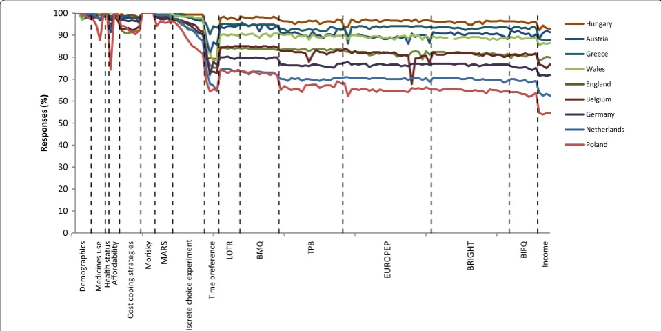
enabling ‘forced answer’ settings within SurveyMonkey. Figure 1 presents the percentage of complete responses by question, and in the order the questions were asked. A dip is seen at the open ended time preference meas-ure, which may be perceived as cognitively challenging [23]. The sensitivity of information requested on income explains the final dip in the plot. Missing data was assumed to be MAR. We consider the impact of possible departures from MAR in the discussion.

We chose to impute each country-specific data set sep-arately, as associations between variables were expected to differ between countries.

A complete MI prediction equation results in 134 pre-dictors for each incomplete variable. Some categorical variables had categories with low observed frequency which presented additional challenges. These were han-dled by collapsing response categories. Taking education as an example, in Greece, 52.3 % received primary educa-tion as a highest educaeduca-tional attainment, 29.0 % second-ary education and 18.7 % higher education. For England the corresponding figures were 0.3, 33.7 and 65.3  % respectively. We collapsed the lower two categories, conducting the final analysis on ‘up to secondary educa-tion’ and ‘higher educaeduca-tion’. Collapsing of categories was applied to all data sets, and was maintained for analysis.

Within the income section of the survey, questions had an ‘opt out’ response if respondents were unwilling to provide the information. Additional file 1: Table S1 sum-marises these responses across the nine countries. Ques-tions in this section took an ordered categorical format, which we were keen to preserve (rather than impute as nominal variables). This was achieved by generating two separate variables for each income item. An initial binary variable reflected whether the respondent was willing to provide a response. An ordinal variable then reflected the response, conditional on the respondent being willing to provide the information.

The number of imputations, M, was chosen based upon analysis of the Polish data set, which was received 3 months prior to data from other countries. For this data set 26 % of response values were missing, so the number of imputations was set at M = 25, closely reflecting the suggestion of one imputation per percent missing data [1]. For subsequent country-level data sets the amount of missing data was in fact lower, 5–22 %, but M = 25 was maintained for consistency.

Initially a full imputation model was attempted for this data, but failed to converge for all imputations. Apply-ing our proposed approach, model size depended on the number of items within each subscale (range, 56–72).

Demographics Medicines use Health statu

s

Affordabilit

y

Cost coping strategies

Morisky MARS

Discrete choice experiment

Time preferenc

e

LOT

R

BM

Q

TP

B

EUROPE

P

BRIGHT

BIPQ

Income

0 10 20 30 40 50 60 70 80 90 100

Responses

(%

)

Hungary Austria Greece Wales England Belgium Germany Netherlands Poland

Fig. 1 Responses rate by question and country. Questions not-applicable due differences in healthcare systems appear as breaks in the plot. MARS

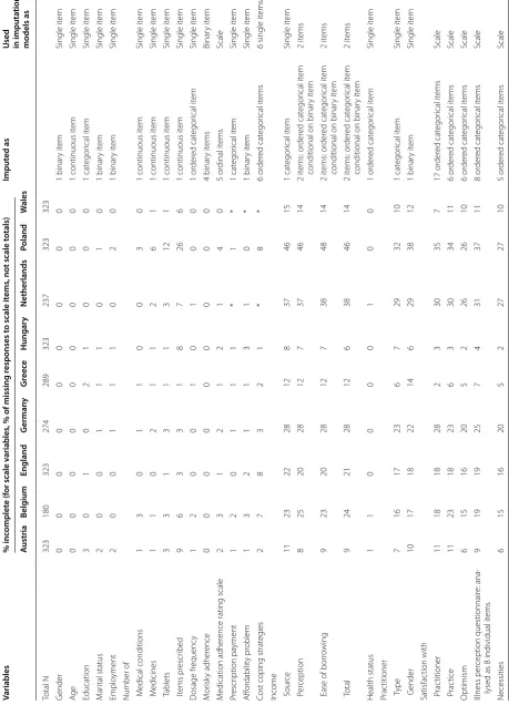
Each prediction equation included the demographic vari-ables and the primary outcome measure. MI was con-ducted using the -ice- routine in Stata 10 [19, 24, 25]. Categorical variables were handled using -mlogit- and -ologit- [25]. Subscale totals were calculated following each cycle of the imputation using the passive option of the -ice- routine. The final imputation methods and mod-els used to impute different parts of the survey are sum-marised in Table 1, with an extract of Stata code provided in Additional file 2: Appendix S1.

Data analysis

Primary analysis was to be conducted by country, and the survey was powered as such. The primary analy-sis was a logistic regression with Morisky score as out-come, aiming to identify predictors of non-adherence to medication. There were deemed to be too many pre-dictors to enter into the model, N = 42 (Table 1), there-fore an initial variable selection step was employed. For the regression results presented here, we have used the same pragmatic variable selection as in the main analysis [21]: continuous variables were selected using univari-ate tests, pooled using Rubin’s rules; cunivari-ategorical variables were selected using Chi squared tests and ANOVA on complete case data; and variables relating to numbers of medicines were selected using t-tests controlling for age on complete case data. Variables showing univariate sig-nificance with the outcome measure were entered into the regression model.

We also compared variable selection using complete case data with variable selection procedure using Rubin’s rules in the pooled MI data, using unadjusted or age-adjusted analyses as described above [20, 26].

Simulation

We devised a simulation study to impartially assess the performance of the new method against some alterna-tives in a realistic setting—based on the case study.

We invoked a simpler set up than the case study, to allow comparison of the proposed strategy with a full imputa-tion model, which is not possible on the full data set. The variables included were Morisky score (fully observed), age in years (fully observed), attitude (partially observed, the sum of seven items, scored as integers from 1 to 5) and

practitioner satisfaction (partially observed, the sum of 17

items, also integers from 1 to 5). We estimated four quan-tities: the means of attitude and practitioner satisfaction, and their coefficients in a logistic regression of Morisky score on age, attitude and practitioner satisfaction.

Simulation procedure

The simulation procedure was as follows for 1000 replications:

• 323 observations of the 26 variables (Morisky score, age, 7 items of attitude, 17 items of practitioner sat-isfaction) were simulated from a multivariate normal distribution based on the observed vectors of means and standard deviations and the observed correlation matrix.

• Morisky score was rounded to the nearest of 0 or 1. Items making up attitude and practitioner satisfac-tion were rounded to take values of 1–5.

• Missing values were introduced for items of the atti-tude and practitioner satisfaction scales. The prob-ability of missing data depended on Morisky score and age, based on the real dataset (MAR). Each observation was assigned to one of three categories: all items observed, some items observed, or no items observed. Three scenarios are simulated:

– _{Base case: 35 % had all items missing for a scale;} 8 % had one or two items missing.

– _{More incomplete observations with partial data:} 18 % had all items missing for a scale; 25 % had one or two items missing.

– _{Fewer observations with complete data: 55 % had} all items missing for a scale; 15 % had just one or two missing.

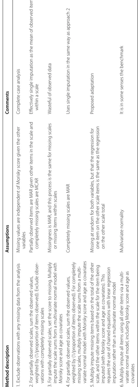
For each simulated dataset six methods were con-sidered for dealing with the missing data, presented in Table 2. Ten imputations were used for all MI-based approaches.

Outcomes

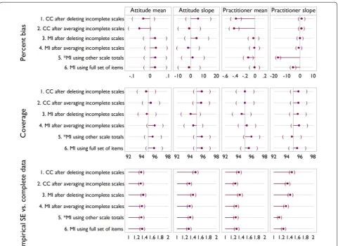
For each parameter of interest we summarise percent bias (compared to analysis of complete data), coverage, and efficiency (through the empirical standard error, expressed by comparison to method 1) over the 1000 replications for that scenario. Estimates are accompanied by Monte-Carlo 95 % confidence intervals.

Results Case study

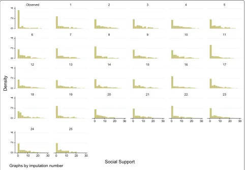
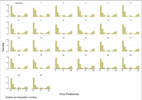
To compare the performance and fit of the MI models, we plot complete case data versus imputed data, overall and by imputation. Figures 2 and 3 illustrate such com-parisons for the individual item and scale total which dis-played the highest proportion of missing data. These are one of the time preference variables (36 % missing data), and the support scale (70 % of scale totals missing, 43 % individual items missing), both from the Polish data set. On inspection, in both cases, the imputed data is similar but not identical to the complete case data.

Table 1 M issing da ta b y c oun tr y, and ho

w it w

as handled in imputa

tion mo dels Variables % inc omplet e (f

or scale v

ariables

, % of missing r

esponses t

o scale it

ems

, not scale t

otals)

Imput

ed as

U

sed _in imputa

tion models as A ustria Belg ium England G erman y G re ece Hungar y Netherlands Poland W ales Total N 323 180 323 274 289 323 237 323 323 G ender 0 0 0 0 0 0 0 0 0 1 binar y it em Single it em Ag e 0 0 0 0 0 0 0 0 0

1 continuous it

em Single it em Education 3 0 1 0 2 1 0 0 0 1 cat egor ical it em Single it em M ar ital status 2 0 0 1 1 1 0 1 0 1 binar y it em Single it em Emplo yment 2 0 0 1 1 1 0 2 0 1 binar y it em Single it em

Number of M

edical conditions 1 3 0 1 1 0 0 3 0

1 continuous it

em Single it em M edicines 1 1 0 2 1 1 2 6 1

1 continuous it

em Single it em T ablets 3 3 1 3 1 1 3 12 1

1 continuous it

em Single it em I tems pr escr ibed 9 6 3 3 1 8 7 26 6

1 continuous it

em Single it em D osage fr equenc y 1 2 0 0 1 0 1 0 0 1 or der ed cat egor ical it em Single it em M or isk y adher ence 0 0 0 0 0 0 0 0 0 4 binar y it ems Binar y it em M edication adher

ence rating scale

2 3 1 2 1 2 1 4 0 5 or dinal it ems Scale Pr escr iption pa yment 1 2 0 1 1 1 * 1 * 1 cat egor ical it em Single it em A ffor dabilit y pr oblem 1 3 2 1 1 3 1 0 * 1 binar y it em Single it em

Cost coping strat

eg ies 2 7 8 3 2 1 * 8 * 6 or der ed cat egor ical it ems

6 single it

ems

Income Sour

ce 11 23 22 28 12 8 37 46 15 1 cat egor ical it em Single it em P er ception 8 25 20 28 12 7 37 46 14 2 it ems: or der ed cat egor ical it em

conditional on binar

y it

em

2 it

ems

Ease of bor

ro wing 9 23 20 28 12 7 38 48 14 2 it ems: or der ed cat egor ical it em

conditional on binar

y it em 2 it ems T otal 9 24 21 28 12 6 38 46 14 2 it ems: or der ed cat egor ical it em

conditional on binar

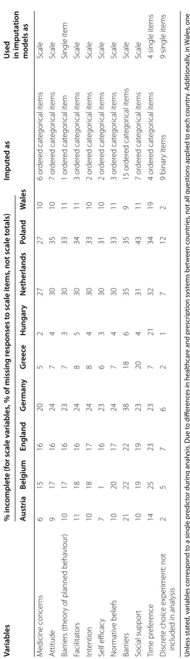
y it em 2 it ems Health status 1 1 0 0 0 0 1 0 0 1 or der ed cat egor ical it em Single it em Prac titioner T ype 7 16 17 23 6 7 29 32 10 1 cat egor ical it em Single it em G ender 10 17 18 22 14 6 29 38 12 1 binar y it em Single it em Satisfac tion with P rac titioner 11 18 18 28 2 3 30 35 7 17 or der ed cat egor ical it ems Scale P rac tice 11 23 18 23 6 3 30 34 11 6 or der ed cat egor ical it ems Scale Optimism 6 15 16 20 5 2 26 26 10 6 or der ed cat egor ical it ems Scale Illness per ception questionnair e: ana

-lysed as 8 individual it

Table 1 c on tinued Variables % inc omplet e (f

or scale v

ariables

, % of missing r

esponses t

o scale it

ems

, not scale t

otals)

Imput

ed as

U

sed _in imputa

tion models as A ustria Belg ium England G erman y G re ece Hungar y Netherlands Poland W ales M edicine concer ns 6 15 16 20 5 2 27 27 10 6 or der ed cat egor ical it ems Scale A ttitude 9 17 16 24 7 4 30 35 10 7 or der ed cat egor ical it ems Scale Bar riers (theor

y of planned beha

viour) 10 17 16 23 7 3 30 33 11 1 or der ed cat egor ical it em Single it em Facilitat ors 11 18 16 24 8 5 30 34 11 3 or der ed cat egor ical it ems Scale Int ention 10 18 17 24 8 4 30 33 10 2 or der ed cat egor ical it ems Scale Self efficac y 7 1 16 23 6 3 30 31 10 2 or der ed cat egor ical it ems Scale Nor mativ e belief s 10 20 17 24 7 4 30 33 11 3 or der ed cat egor ical it ems Scale Bar riers 21 22 22 38 18 6 35 35 9 15 or der ed cat egor ical it ems Scale Social suppor t 10 19 19 23 20 4 31 43 11 7 or der ed cat egor ical it ems Scale Time pr ef er ence 14 25 23 23 7 21 32 34 19 4 or der ed cat egor ical it ems

4 single it

ems

Discr

et

e choice exper

iment: not

included in analysis

2 5 7 6 2 1 7 12 2 9 binar y it ems

9 single it

ems Unless sta ted , v ar iables c or respond t

o a single pr

edic tor dur ing analy sis . D ue t o diff er enc

es in healthcar

e and pr

escr iption sy st ems bet w een c oun tr ies

, not all questions applied t

o each c

oun tr y. A dditionally , in W ales , one question fr

om the bar

riers scale w

as not applicable

, thus this scale has only 14 it

ems

. W

hilst illness per

ception questions w

er

e imput

ed as scale it

ems

, they w

er

e analy

sed individually

* V

ar

iables not analy

sed due t

o diff

er

enc

es in pr

escr

Table 2 Summar y of metho ds c ompar ed in simula tion M ethod description A ssumptions Commen ts 1. Ex clude obser

vations with an

y missing data fr

om the analysis

M

issing values ar

e independent of M

or

isk

y scor

e g

iv

en the other

var

iables

Complet

e case analysis

2. F

or par

tially obser

ved scales

, sum the obser

ved values , w eight ed b y (1/pr opor

tion of it

ems obser

ved). Ex

clude obser

-vations with complet

ely missing scales

Par tially obser ved it ems ar e M AR g iv

en other it

ems in the scale and

complet

ely missing scales ar

e MCAR

Eff

ec

tiv

ely single imputation as the mean of obser

ved it

ems

within a scale

3. F

or par

tially obser

ved scales

, set the scor

e t

o missing

. M

ultiply

imput

e the scale sums fr

om a multivar

iat

e nor

mal model with

M

or

isk

y scor

e and age as co

var

iat

es

M

issing

ness is M

AR, and this pr

ocess is the same f

or missing scales

or missing it

ems within scales

W

ast

eful of obser

ved data

4. F

or par

tially obser

ved scales

, sum the obser

ved values , w eight ed b y (1/pr opor

tion of it

ems obser

ved). F

or complet

ely

missing scales

, multiply imput

e the scale sums fr

om a multi

-var

iat

e nor

mal model with M

or

isk

y scor

e and age as co

var

iat

es

Complet

ely missing scales ar

e M

AR

Uses single imputation in the same wa

y as appr

oach 2

5. M

ultiply imput

e missing it

ems based on the t

otal of the other

scale

, and the other it

ems within the scale f

or the it

em being

imput

ed (with M

or

isk

y scor

e and age as co

var

iat

es).

This

requir

es the use of chained equations with linear r

eg

ression

imputation rather than a multivar

iat

e nor

mal model

M

issing at random f

or both var

iables

, but that the r

eg

ression f

or

one it

em on the other scale it

ems is the same as the r

eg

ression

on the other scale t

otal

Pr

oposed adaptation

6. M

ultiply imput

e all it

ems using all other it

ems via a multi

-var

iat

e nor

mal model

, including M

or

isk

y scor

e and age as

co var iat es M ultivar iat e nor malit y

It is in some senses the benchmar

results are illustrated as odds ratios with 95  % confi-dence intervals in Fig. 4. Differences in the significance of results are observed between data analysed using MI and CC for age, barriers and personal control in Aus-tria, barriers and self-efficacy in England, barriers and employment in Poland and age in Wales. The majority of differences (except barriers in Austria and Poland) are attributable to narrower confidence intervals in the MI analysis, thus illustrating the higher power and efficiency which the MI approach offers. Whilst differences in the standard errors alter the significance of the results, there are no substantial differences in the point estimates of the β-coefficients.

Table 3 presents the proportional reduction in stand-ard error for MI compared to CC analysis, summarised for all variables entered in the country level regression analyses. From the table, it can be seen that on average, standard error is reduced by 39 % when an MI approach is adopted over CC analysis. Standard errors are smaller for MI than CC analysis for all variables other than ill-ness coherence in Belgium (where there was no change in standard error between MI and CC). To ensure that

reduction in standard error was not biased by variable selection method, reduction was also compared for ables selected using CC and MI approaches. For vari-ables selected using the CC method, mean standard error reduction was 45 % (95 % CI: 12, 78 %; range 15–99.9 %). For variables selected using the MI method, mean stand-ard error reduction was 34 % (95 % CI: 11, 58 %; range 2–57 %).

For the univariate variable selection, disparity between which variables were selected using either the MI or CC approach is summarised in Table 4. Chi squared tests indicate that the disparity was significant, (χ2 _{=  250,}

p  <  0.001), with agreement (sum of the main diagonal) achieved for only 92.5 % of variables. Lower agreement is observed in the variables with more missing data: at <20 % missing data agreement was 94 %, compared to 88 % when missing data was > 20%.

Simulation

Figures 5, 6 and 7 show the results of the simulation for the three scenarios. In the base case Fig. 5, signifi-cant downward bias is seen for the mean of practitioner

0

.2

.4

0

.2

.4

0

.2

.4

0

.2

.4

0

.2

.4

0 10 20 30 0 10 20 30 0 10 20 30 0 10 20 30

0 10 20 30 0 10 20 30

Observed 1 2 3 4 5

6 7 8 9 10 11

12 13 14 15 16 17

18 19 20 21 22 23

24 25

De

ns

ity

Social Support Graphs by imputation number

satisfaction, for methods 1, 2 and 5, with methods 5 and 6 showing significant bias on the slope. In terms of cov-erage, there are no significant differences between meth-ods. Empirical standard error also shows little variability between methods, except that it is lower for method 5 on slope for practitioner satisfaction. This reflects the down-ward bias.

Increasing the number of incomplete observations with partial data, as in scenario 2 (Fig. 6) or increasing the number of incomplete observations (Fig. 7) indicate a similar story. Methods 1 and 2 show an increase in bias compared to the base case, with method 4 showing sig-nificant downward bias and reduced coverage for TPB slope in both scenarios. In both scenarios the empiri-cal standard error appears lower than for the base case, reflecting downward bias.

Overall, method 6 is seen to be the best, broadly exhib-iting the least bias and the most efficiency, and we regard it as a benchmark. This method is not always feasible however, for example in the case study described above. Method 1 often displays a large amount of bias, and like method 3, is inefficient and wasteful of observed data.

Method 2 indicates bias in all bar the base case, and may artificially reduce variability due to being effectively sin-gle imputation.

It appears therefore from the simulations and assump-tions that in terms of bias, coverage and empirical stand-ard error that method 4 or 5 would be best in cases where method 6 is not feasible. At this point it is unclear which of the two methods is most appropriate, method 4, sim-ilar to method 2 is akin to a single imputation, and for method 5 whilst the assumptions seem more appropriate, the simulation evidence suggests it can introduce bias when these are violated.

Discussion

Our proposed method for handling multiple multi-item scales allows imputation of individual items by using scale totals within the imputation models, such that given primary outcome p, scale T and demographics d1

… dn, item s1 from scale S, is imputed using p, d1 … dn,

s2 … sn and summary score t. The use of summed scale

scores within the predictor equations reduces both the number of predictors in each equation and the sparsity

0

.2

.4

0

.2

.4

0

.2

.4

0

.2

.4

0

.2

.4

0 5 10 0 5 10 0 5 10 0 5 10

0 5 10 0 5 10

Observed 1 2 3 4 5

6 7 8 9 10 11

12 13 14 15 16 17

18 19 20 21 22 23

24 25

Densit

y

Time Preference

Graphs by imputation number

in the data set. This approach facilitates the efficient use of MI in large survey data sets with multiple multi-item scales. Using MICE allows preservation of the structure of the data, in terms of point estimates and variance or variables, and covariance. Should the approach presented here still result in overly complex prediction equations, a

further simplification would be to replace s2 … sn in the

prediction equation by their sum or average.

For subscales of the health psychology measures, rather than to impute every individual item, one simplifica-tion of our method would be to impute only the totals of the subscales. For our data this would reduce the size of the model from 134 to 56 predictors per variable. A disadvantage of this approach, however, is that it would restrict analysis to summed scales, leaving no scope for exploring individual items.

Forming scale totals prior to imputation, and then imputing missing totals is a further simplification, but comes with an additional disadvantage: for those respondents who have completed some, but not all, of the items in a subscale, those responses are discarded, or imputed by an ad-hoc method such as using the mean of observed items. Taking as an example the 17-item practitioner satisfaction scale in the Austrian data set, 262 respondents (from 323) completed all items. The response rate to individual items ranged from 278 to 292 responses, and the above approach would discard a total of 437 responses, collected from 31 respondents, from this scale.

Our simulation study compares these alternatives with a benchmark ‘complete’ MI analysis, and complete case Austria

Belgium England Germany Netherlands Poland Wales

.9 1 1.1

Age

Austria

England

Greece

Hungary

Poland

Wales

1 1.1 1.2 1.3

Barriers

Austria

England

Germany

Hungary

Poland

Wales

5 10 20

Employment

Austria

England

Greece

Hungary

Wales

.5 .7 .9 1.1

Personal Control

Austria Belgium England Germany Greece Hungary Netherlands Poland Wales

.4 .8 1.2

Self Efficacy

MI CC

Fig. 4 Forest plots illustrating odds ratios from the logistic regression

Table 3 Summary of  proportional decrease in  standard error, between  complete case and  multiple imputation analyses

Mean (%) Min (%) Max (%) Median

(%) Standard deviation

(%)

Overall 39 0 100 38 19

Austria 38 22 55 38 8

Belgium 5 0 13 4 5

England 58 33 100 45 27

Germany 21 12 26 22 5

Greece 50 43 58 50 4

Hungary 23 14 27 23 4

Nether-lands 29 24 36 29 4

Poland 41 14 59 42 12

alternatives. Results from the simulation indicate that simplification by averaging incomplete scales and our proposed method perform comparably, with the simpli-fication reducing model complexity, compromised with a slight loss of efficiency. Complete case methods were seen to perform poorly, with an increase in bias, par-ticularly when the amount of missingness was increased. This result is consistent with a previous study on multi-item imputation, where mean imputation and single

imputation were shown to have larger bias and worse coverage than item level multiple imputation, and com-plete case analysis was shown to overestimate standard error and reduce power [16].

Certain limitations are acknowledged. Typically, analy-sis with MI relies on an assumption of data being MAR. This assumption cannot be proven, but for large well-conducted surveys, the assumption of MAR is often con-sidered a reasonable starting point for statistical analysis. Table 4 Disparity in variable selection between CC and MI, over 42 variables in 9 countries

χ2_{= 250, p < 0.001}

Complete case method

Included n (%) Excluded n (%) Total

Multiple imputation Included n (%) 86 (23) 3 (1) 89

Excluded n (%) 25 (7) 259 (69) 284

Total 111 262 373

Rubin et  al. conclude that whilst assuming MAR may be inadequate if there are high levels of missingness or insufficient relevant covariates, “the evidence seems to be that at least in some carefully designed survey contexts, modelling observed data under MAR can provide accept-able answers” [27].

A further limitation of the proposed method for han-dling multiple multi-item scales is the assumption that items from different scales are only correlated via the scale totals. The majority of scales and measures used in this survey are validated, and were tested during analysis for internal consistency. Additionally, as the survey was structured such that each measure was presented in its entirety, independently, this a plausible assumption for our data.

During data analysis, significant univariate differ-ences were observed between CC and MI which indi-cate that performing variable selection on different data sets would result in the entry of different variables into

the regression model. In comparison with CC, using the same variables for both approaches, regression results from MI show standard error to be reduced by an average of 39  %, with no cases where standard error increases, thus resulting in more precise conclusions.

Data collection will almost always result in missing data. It is the duty of researchers and analysts to firstly minimise the extent of missing data by ensuring appro-priate methods for enhancing data capture are imple-mented, but also to handle missingness in a way best suited to the data and research question. Poor handling and reporting of missing data may result in misleading conclusions and are one of the main reasons for publica-tion rejecpublica-tions [28, 29]. With the advent of MI routines in SPSS, R, SAS and Stata, MI is now readily accessible to analysts as a robust method for handling missing data, which can be applied in a number of contexts [4].

Alongside our proposed adaptation for imputing multi-ple multi-item scales, ordinal regression and conditional

imputation are also powerful tools which, in this study, have allowed us to address the challenges presented by large scale survey data. Our proposed adaptation makes MI practical for large scale survey data, where a full pre-diction model may be infeasible, and we have shown that the use of MI in this way makes better use of available data and can yield substantively different results from simpler techniques.

Authors’ contributions

DH conceived the research. CP, IW contributed to the design, analysis and interpretation of data. TM designed and implemented the simulation study, CP drafted the article and all authors revised it critically for important Additional files

Additional file1. Stata code.

Additional file 2. Responses to income questions.

intellectual content, and gave their final approval of the version to be pub-lished. All authors read and approved the final manuscript.

Author details

1 _{Centre for Health Economics and Medicines Evaluation, Bangor University,} Ardudwy, Normal Site, Holyhead Road, Bangor, Gwynedd LL57 2PZ, UK. 2 _MRC Clinical Trials Unit at UCL, Institute of Clinical Trials and Methodology, Aviation House, 125 Kingsway, London WC2B 6NH, UK. 3 _{London School of Hygiene} and Tropical Medicine, Keppel Street, London WC1E 7HT, UK. 4 _MRC Biostatis-tics Unit, Cambridge Institute of Public Health, Robinson Way, Cambridge CB2 0SR, UK.

Acknowledgements

We are grateful to Emily Fargher, Dr Valerie Morrison, Dr Sahdia Parveen and other members of the ABC Project Team for their support on this project. Competing interests

The authors declare that they have no competing interests. Funding

• We accept pre-submission inquiries

• Our selector tool helps you to find the most relevant journal

• We provide round the clock customer support

• Convenient online submission

• Thorough peer review

• Inclusion in PubMed and all major indexing services

• Maximum visibility for your research

Submit your manuscript at www.biomedcentral.com/submit

Submit your next manuscript to BioMed Central

and we will help you at every step:

number G0800792. IW was supported by the Medical Research Council [Unit Programme number U105260558].

Role of the funder

The funder had no role in the study design; in the collection, analysis, and interpretation of data; in the writing of the report; or in the decision to submit the paper for publication.

Received: 17 December 2015 Accepted: 12 January 2016

References

1. White IR, Royston P, Wood AM. Multiple imputation using chained equa-tions: issues and guidance for practice. Stat Med. 2011;30(4):377–99. 2. Wayman JC. Multiple imputation for missing data: What is it and how can

I use it? In Proceedings of the Annual meeting of the American Educa-tional Research Association Chicago, Il. 2003.

3. Baraldi AN, Enders CK. An introduction to modern missing data analyses. J Sch Psychol. 2010;48:5–37.

4. Roth PL. Missing Data: a conceptual review for applied psychologists. Personnel Psychology. 1994;41(3):537–60.

5. Wood A, White IR, Thompson SG. Are missing outcome data adequately handled? a review of published randomized controlled trials in major medical journals. Clin Trials. 2004;1:368–76.

6. Peugh JL, Enders CK. Missing data in educational research: a review of reporting practices and suggestions for improvement. Rev Educ Res. 2004;74(4):525–56.

7. Little RJA. Missing-data adjustments in large surveys. J Bus Econ Stat. 1988;6(3):287–96.

8. Sinharay S, Stern HS, Russell D. The use of multiple imputation for the analysis of missing data. Psychol Methods. 2001;6(4):317–29. 9. Sterne JAC, White IR, Carlin JB, et al. Multiple imputation for missing

data in epidemiological and clinical research: potential and pitfalls. BMJ. 2009;338:b2393.

10. Noble SM, Hollingworth W, Tilling K. Missing data in trial-based cost-effectiveness. analysis: the current state of play. Health Econ. 2012;21(2):187–200.

11. Rousseau M, Simon M, Bertrand R, et al. Reporting missing data: a study of selected articles published from 2003-2007. Qual Quant. 2012;46(5):1393–406.

12. Karahalios A, Baglietto L, Carlin JB, et al. A review of the reporting and handling of missing data in cohort studies with repeated assessment of exposure measures. BMC Med Res Methodol. 2012;12:96.

13. Eekhout I, de Boer MR, Twisk JWR, et al. Missing Data: a systematic review of how they are reported and handled. Epidemiology. 2012;23(5):729–32. 14. Bell ML, Fiero M, Horton NJ, et al. Handling missing data in RCTs; a review

of the top medical journals. BMC Med Res Methodol. 2014;14:118. 15. Simons CL, Rivero-Arias O, Yu LM, et al. Multiple imputation to deal with

missing EQ-5D-3L data: should we impute individual domains or the actual index? Qual Life Res. 2015;24:805–15.

16. Eekhout I, de Vet HCW, Twisk JWR, et al. Missing data in a multi-item instrument were best handled by multiple imputation at the item score level. J Clin Epidemiol. 2014;67:335–42.

17. van Buuren S, Oudshoorn CGM. Multiple imputation by chained equa-tions: MICE V1.0 user’s manual. TNO Report PG/VGZ/00.038. TNO Preven-tie enGezondheid: Leiden (2000). http://www.multiple-imputation.com/

Accessed 26 Nov 2012.

18. White IR, Daniel R, Royston P. Avoiding bias due to perfect prediction in multiple imputation of incomplete categorical variables. Comput Stat Data Anal. 2010;54:2267–75.

19. Royston P. Multiple imputation of missing values: update. Stata J. 2005;5(2):188–201.

20. Rubin DB. Multiple imputation for nonresponse in surveys. New York: Wiley; 1987.

21. Morrison VL, Holmes EAF, Parveen S, et al. Predictors of self-reported adherence to antihypertensive medicines: a multi-national, cross-sec-tional survey. Value Health. 2015. doi:10.1016/j.val.2014.12.013. 22. Morisky DE, Ang A, Krousel-Wood M, et al. Predictive validity of a

medica-tion adherence measure for hypertension control. J Clin Hypertens. 2008;10(5):348–54.

23. van der Pola M, Cairns J. Comparison of two methods of eliciting time preference for future health states. Soc Sci Med. 2008;67(5):883–9. 24. Royston P. Multiple imputation of missing values: update of ice. Stata J.

2005;5(4):527–36.

25. Royston P. Multiple imputation of missing values: further update of ice, with an emphasis on categorical variables. Stata J. 2009;9(3):466–77. 26. Wood AM, White IR, Royston P. How should variable selection be

per-formed with multiply imputed data? Stat Med. 2008;27:3227–46. 27. Rubin DB, Stern HS, Vehovar V. Handling, “don’t know” survey responses:

the case of the slovenian plebiscite. J Am Stat Assoc. 1995;90:822–8. 28. Fernandes-Taylor S, Hyun JK, Reeder RN, et al. Common statistical and

research design problems in manuscripts submitted to high-impact medical journals. BMC Res Notes. 2011;4:304.