Technological Progress, Time Perception and
Environmental Sustainability
Evangelos V. Dioikitopoulos, Sugata Ghosh and Eugenia Vella
ISSN 1749-8368
SERPS no. 2016002
Technological Progress, Time Perception,
and Environmental Sustainability
Evangelos V. Dioikitopoulos, Sugata Ghosh
y, and Eugenia Vella
zJanuary 20, 2016
Abstract
This paper explores the relationship among technological progress, environment and growth by combining endogenous e¢ ciency of public abatement with endogenous dis-counting. Our model can feature two di¤erent balanced growth paths corresponding to di¤erent levels of environmental quality, which remains constant in the long-run although the economy grows. The multiple equilibria point to a non-monotonic relationship among technological progress, growth and the environment, as observed in the data. A Ramsey planner can implement the good equilibrium; however, under a positive technology shock, the economy achieves higher long-run growth at the cost of lower environmental quality (even if agents value the environment highly). This …nding could help us explain why some advanced economies may not succeed in cleaning the environment e¤ectively.
JEL classi…cation: D90, E21, E62, H31, O44, Q28.
Keywords: Time preference, growth, environmental quality, …scal policy, technolog-ical progress.
Acknowledgments:We have bene…ted from comments and suggestions by J. Caballé, K. Neanidis, S. Kalyvitis, M. Gil Molto, A. Navas, T. Xepapadeas, R. Wendner; and feedback from participants at the JPET 2014 conference in Seattle, and the audience at the research seminar presentation in Graz in 2014. The usual disclaimer applies.
Department of Management, King’s College London, UK. e-mail: [email protected]
yDepartment of Economics and Finance, Brunel University London, Uxbridge, UB8 3PH, UK. e-mail: [email protected]
1
Introduction
The link between economic growth and the environment is generally complex, and is often
shaped by economic (notably …scal) policy. It is well known that, across time, economic growth
has a negative relation with environmental quality in the early stages of development, which
tends to get reversed beyond a point (Grossman and Krueger, 1995; Millimet, List and Stengos,
2003; Varvarigos, 2014).1 But across countries, advanced economies on average perform better
in terms of growth and environmental quality, while developing countries often stagnate with low
growth and low environmental quality (Fact 1). Interestingly, however, fast-growing economies
could actually end up polluting the environment, ex post, despite there being increases in total
factor productivity (TFP), which could have been utilised to …nance pollution abatement (Fact
2).2
Using a uni…ed framework, we attempt to explain those facts and examine the
associ-ated policy implications. First, we consider endogenous discounting of utility, which depends
on environmental quality. A time-varying, rather than constant, discount rate is important
for the evaluation of long-run projects, in particular when future generations are taken into
consideration (Hepburn, Koundouri, Panopoulou and Pantelidis, 2009, and Freeman, Groom,
Panopoulou and Pantelidis, 2015). In our case, better environmental quality increases the
pref-erences for the future relative to the current period, raises savings and growth and, in turn,
the resources to abate pollution activities. On the ‡ip side, there exists a vicious cycle of high
discount rate, low savings, low environmental quality and low growth. We take into account
the factors that help us to explain Fact 1, which are about the existence of those two equilibria
in a decentralized set-up; second, we consider endogenous (optimal) …scal policy, which enables
the ‘bad’ equilibrium (low growth and low environmental quality) to be eliminated. At the
same time, we show that under increases in TFP, it is possible for some advanced economies
1An interesting observation made by Beckerman (1992) was that the “way to attain a decent environment
in most countries is to become rich”!
2To provide a concrete example, if we take the case of China, although its income per capita and growth rate
to perform badly in terms of the environment (while pursuing a welfare-maximizing policy), as
this is illustrated by Fact 2.
In particular, we consider a competitive market with …rms producing output using private
and public capital. The latter could be interpreted as infrastructure, traditional or ‘green’.
Public capital is …nanced through income taxation to pay for the spending on infrastructure
and abatement, as in Economides and Philippopoulos (2008), Ray Barman and Gupta (2010),
Vella, Dioikitopoulos and Kalyvitis (2015). The stock of environmental quality, which evolves
through time but remains constant in the long-run (Eliasson and Turnovsky, 2004), depends
negatively on pollutants and positively on abatement expenditures, which are undertaken by
governments to bring about improvements in environmental quality. This feature is present in
a number of papers like Mohtadi (1996), Smulders and Gradus (1996), Byrne (1997), Liddle
(2001), Bretschger and Smulders (2006), Managi (2006), among others.
Environmental degradation occurs via aggregate consumption, which is the source of
pol-lution.3 This is a realistic assumption, given that consumption of natural resources and the
consumption of energy-intensive luxury goods are important sources of pollution.
Consump-tion of automobile services (particularly when vehicles are without well-funcConsump-tioning catalytic
converters) leads to signi…cant air pollution. Household wastes and municipal sewage, when
dumped into waterways, lead to widespread water pollution. Consumption of various electronic
appliances leads to radiation and sound pollution. These are all by-products of consumption
activities. Other examples include the consumption of fossil fuels like coal, wood, kerosene
oil, etc., in the rural areas of developing countries. Some of the existing literature adopts this
consumption-caused pollution hypothesis.4 The dynamics of environmental quality, which is a
function of pollution, evolve along the lines of Jouvet, Pestieau and Ponthiere (2010).
As regards environmental preservation, a distinct feature of our model is that the
e¤ective-3This is in contrast to models that consider physical capital as the source of pollution: see, for example,
Bovenberg and Smulders (1995), Elbasha and Roe (1996), Smulders and Gradus (1996), Byrne (1997), Cassou and Hamilton (2004), Benarroch and Weder (2006), Itaya (2008), Pautrel (2009), and Chu, Lai and Liao (2015).
4See the contributions of John and Pecchenino (1994), Howarth (1996), Liddle (2001), Egli and Steger (2007),
ness of public abatement expenditure is enhanced by the amount of infrastructure per unit of
output.5 To this end, one can cite examples of investment in green infrastructure projects, e.g.,
e¢ cient management of stormwater, climate adaptation and provision of green space, which
can supplement the direct bene…ts from abatement.6 Public spending on human capital
accu-mulation that could enable the educated to carry out R&D activities to bolster the environment
is yet another example of this phenomenon.
We consider, …rst, the workings of a decentralized economy where the government takes the
tax rate and the proportion of spending on infrastructure vis-a-vis abatement as given, and then
the case of a benevolent government that formulates its …scal policy optimally (i.e., chooses its
instruments: the tax rate and the proportion of spending on abatement to maximize agents’
welfare. The latter case of an optimizing government is one where the Ramsey …scal policy is
pursued to attain the second-best scenario.
Our results for the decentralized economy show, interestingly, that there emerge multiple
(two) equilibria: one, a ‘bad’, low-growth, equilibrium, and the other, a ‘good’, high-growth,
equilibrium. The former typi…es the case of a resource-poor country, with consumers having a
high degree of impatience and high consumption propensity, which, in addition to low growth
also results in high pollution and low environmental quality. Exactly the opposite holds for
the other equilibrium, the prototype of an advanced economy, characterized by a low rate of
time preference, low consumption-to-capital ratio, low pollution, good environmental quality
and high growth. Our …ndings can be compared with Schumacher (2009) where multiplicity of
steady states occurs since when an agent is very poor, then increases in consumption are
neces-sary for survival, and the agent is so impatient that the preferences are clearly directed towards
the current period. By contrast, when overall wealth has already been built up su¢ ciently, the
5Governments …nance a variety of enviornmental protection activities (public abatement). The proportion
of government expenditure in total expenditure on abatement is relatively high in many countries (see e.g. Hatzipanayotou, Michael and Lahiri, 2003, and Haibara, 2009).
6See Quaas (2007) for a spatial equilibrium model of an economy - based on stylized facts observed for
discount rate becomes relatively low and people plan ahead for the future.7 We also study the
implications of higher TFP for both equilibria. For the bad equilibrium, despite the higher
out-put, consumption rises more than in proportion, pollution is higher and environmental quality
is lower; the resulting higher degree of impatience contributes to even lower growth.
Under Ramsey …scal policy, by contrast, we no longer have the existence of two feasible
equilibria, but end up with only one equilibrium. The government, by being able to exercise
two additional instruments, other than its overall expenditure, is able to channel the
econ-omy in a direction whereby it can avoid being trapped in the bad equilibrium, so only the
high-growth equilibrium (with good environmental quality) ensures. The implications of
tech-nological progress in this case is to achieve higher output and thereby to strive for ever higher
rates of growth by allocating a higher proportion of government revenues towards infrastructure,
even if this ‘dynamic’objective comes at the cost of some lowering of environmental quality.8
The contribution of our paper is, therefore, threefold. First, it extends the existing literature
on growth, environment and endogenous discounting by providing a uni…ed environmental
law of motion, and taking into account the e¤ect of ‘green’infrastructure on the e¢ ciency of
abatement technology. As distinct from Yanase (2011), in our model environment evolves as
stock, which is more realistic, and this enables us to capture the empirical fact of the existence
of an environmental poverty trap. Also, di¤erently to Vella, Dioikitopoulos and Kalyvitis
(2015), here time preference depends solely on environmental quality, while consumption adds
negatively to environmental preservation. This feature of our model enables us to focus on the
sole e¤ect of environmental quality on time discounting.
Second, we provide an explanation for the poor environmental performance of advanced
countries through a normative aspect (endogenous government policy) by bringing forward the
7By contrast, in Chu, Lai and Liao (2015), despite time preference being endogenous, the decentralised
equilibrium is unique and locally determinate, and there are no transitional dynamics (and the same is true of the social optimum).
8In Economides and Philippopoulos (2008), when citizens care more about the environment, extra revenues
link with TFP. While other models tried to explain the fact the advanced economies have
better performance in terms of envronmental quality, to the best of our knowledge, this is the
…rst paper that shows that under a second-best welfare maximizing policy objective, advanced
countries could end up hurting the environment.
Third, our paper contributes to the literature on endogenous growth and environmental
resources by developing a model in which balanced growth is consistent with constant
environ-mental quality, under explicit modelling of environenviron-mental dynamics and …scal policy. Notably,
unlike Vella, Dioikitopoulos and Kalyvitis (2015), the two balanced growth paths are associated
with di¤erent levels of (constant) environmental quality. Also, Eliasson and Turnovsky (2004)
have emphasized the shortcomings of existing endogenous growth models in generating a
con-stant level of environmental quality in the long-run. They, however, use a simpler framework
that does not consider public environmental policies.
Turning now to real world data, although various trends can be observed our results go
some way towards explaining the situation in high-growth economies like China over the past
decade, where a rise in productivity, higher investment in infrastructure and high growth rates
exist side by side with some decline in the quality of the environment. More speci…cally,
for China, research and development (R&D) expenditure (as % of GDP) rose continuously
over the years (from 1.32 in 2005 to 1.98 in 2012).9 With a decadal growth rate of 10% and
GDP per capita (in current US$) that rose from 1,731.1 in 2005 to 6,807.4 in 2013, a decline
in environmental quality was evident as regard emissions of CO2, methane and N2O. CO2
emissions, for example, went up from 4.4 in 2005 to 6.2 in 2010. In line with the research
conducted in this study, the data from China indicates that policy-induced changes have had
an e¤ect on growth and the environment, with the improvement in technology boosting growth
but depleting the environment to an extent.10
9If, instead of R&D expenditure, we considered other items listed under the "Science & Technology" indicator,
such as researchers in R&D (per million people), then also it can be seen that there was an increase (from 890 in 2010 to 1020 in 2012). Yet another indicator: patent applications (residents), shows the same trend, with such applications increasing about 2.5 times between 2010 and 2013 in China. For India, too, we see a similar trend for this indicator.
10It is more appropriate to link these trends in the data to the Ramsey policy outcome rather than to a pure
The rest of the paper is structured as follows. Section 2 sets up the model. Section 3
solves the optimization problem of households and …rms, and studies the properties of the
decentralized economy. Section 4 analyzes the role of Ramsey government in selecting a
second-best allocation and studies the e¤ect of technological progress on policy instruments. Finally,
section 5 concludes the paper.
2
The model
This section presents the set-up of our closed-economy model. The main features are as follows:
(a) households derive utility from consumption and environmental quality, which has a public
good character; (b) the subjective discount rate is a negative function of environmental quality,
taken as given by the agents; (c) public infrastructure provides production externalities to …rms
and enhances the e¢ ciency of abatement technology; (d) consumption generates environmental
pollution; (e) the government imposes a tax on output and uses the collected tax revenues to
…nance infrastructure and abatement.
2.1
Households
The economy is made up of a large number of identical, in…nitely-lived households, normalized
to unity, and each one seeks to maximize the present discounted value of the lifetime utility:
Z 1
0
u(Ct; Nt) exp
Z t
0
(Nv)dv dt (1)
where u(C; N) = vlnC + (1 v) lnN is the instantaneous utility function with 0 < v 1
measuring how much agents value consumption,C, vis-à-vis the stock of economy-wide natural
resources, interpreted as an index for environmental quality, N. In turn, (N) denotes the
endogenous rate of time preference (RTP), which is assumed to depend negatively on
mental quality, i.e. N 0.11 The assumption, that a higher level of environmental quality
lowers individual impatience, follows Yanase (2011) and captures the well-documented ‘life
ex-pectancy e¤ect’of environmental quality or pollution (see Introduction). Further, we assume
that there exists a lower positive bound for the RTP, denoted by , i.e. lim(N)!0 (N) = >0.
Households save in the form of capital and receive dividends, . The budget constraint of
the household is given by:
_
W +C =rW + (2)
where a dot over a variable denotes a derivative with respect to time,ris the capital rental rate,
W denotes …nancial assets and the initial asset endowment W(0)>0 is given. The household
acts competitively by taking prices, policy, and environmental quality as given. The latter is
justi…ed by the open-access and public good features of the environment. The control variables
are the paths of C and W, so that the …rst-order conditions include the constraint (2) and the
Euler equation below:
_
C
C =r (N) (3)
Notice that environmental quality a¤ects consumption growth positively through the RTP, and
thus plays an implicit ‘productive’role in the economy.
2.2
Firms
The production function of the single good in this economy is given by:
Y =AKaKg1 a (4)
where Y denotes output, 0< a <1denotes the share of physical capital, K, in the production
function, Kg refers to the public capital stock (e.g. infrastructure) and A represents TFP.
Labour endowment is normalized to unity as we assume no population growth.12 The law of
11We retain the equality sign to allow for comparisons with the case of constant RTP.
12This speci…cation follows the strand of endogenous growth theory assuming that the government can invest
motion for the public capital stock is given by:
_
Kg =G KgKg (5)
where Kg denotes the depreciation rate and Gis government investment in public capital. The
initial capital stock Kg(0)>0 is given. The …rm maximizes pro…ts, :
= (1 )Y (r+ K)K (6)
where 0< <1 is a tax rate on output, K is the depreciation rate of private capital, and its
summation withr forms the rental cost of capital. The …rm acts competitively by taking prices
and policy instruments as given. The …rst-order condition equates the marginal productivity
of capital to its rental cost:
r+ k =Aa(1 )
K Kg
a 1
(7)
2.3
Motion of environmental quality
Following Jouvet, Pestieau and Ponthiere (2010), we assume that the stock of environmental
quality evolves over time according to:
_
N = (1 N)N (1 N)N D (8)
where N denotes environmental quality without degradation, D, and N 2 (0;1) is the degree
of environmental persistence. The initial stock N(0) >0 is given.
Environmental degradation,D, is a positive function of pollution emissions, P, and a
neg-ative function of public abatement expenditures, E, i.e. DP(P; E)>0 and DE(P; E)<0:
D =D(P; E) = P
E (9)
where0< 1denotes the e¢ ciency of the abatement technology in alleviating environmental
degradation.13
We further assume thatP occurs as a by-product of consumption:
P =sC (10)
where 0 < s < 1 is a parameter that quanti…es the detrimental e¤ect of consumption on the
environment.14
In the same vein as Andreoni and Levinson (2001), we assume that the e¢ ciency of
expendi-tures to abate the environment depend on the size of the economy and the level of infrastructure.
In particular, we assume that the e¢ ciency of abatement technology is a positive function of
infrastructure stock as a share of total output, Kg
Y :
= Kg
Y =
Kg
Y (11)
where > 0 is the parameter that captures the e¤ect of infrastructure on the e¢ ciency of
abatement. Intuitively, higher public investment on activities pertaining to public infrastructure
complements public expenditures on abatement and makes it possible to clean the environment
in a more e¢ cient way. To take some concrete examples of this, let us consider e¤ective
stormwater management. This involves providing drainage support in urban areas, as without
such e¤orts, water does not in…ltrate the ground due to much of the surface being impervious,
and causes pollution and ‡ooding via runo¤s.15 One can also consider public spending on
education as a public capital good that a¤ects production and at the same time complements
13For papers with publicly …nanced abatement see e.g. Ligthart and van der Ploeg, 1994; Greiner, 2005; Pérez
and Ruiz, 2007; Gupta and Barman, 2010; Vella, Dioikitopoulos and Kalyvitis (2015). An interesting extension for future research would be to model both private and public abatement.
14As in Andreoni and Levinson (2001), Egli and Steger (2007), Gupta and Ray Barman (2009), Mariani,
Perez-Barahona and Ra¢ n (2010), and Michael, Lahiri and Hatzipanayotou (2015), we consider a linear relationship between pollution ‡ows and consumption activities for the sake of simplicity.
15For example, permeable pavements in parks and parking lots, and wetlands for management of stormwater
the abatement e¢ ciency. Such publicly funded education would be expected to make people
intelligent enough to create more technologies to clean the environment, resulting in a unit
spending on abatement to generate even greater bene…ts. As another example, consider public
spending on transport infrastructure. We know that the conditions of roads are adversely
a¤ected by acid rain (potholes and cracks develop periodically). If the government spends to
maintain such roads (and even spends on new roads), while at the same time spending on
abatement (i.e., spending on research to tackle the causes of acid rain and lessen its harmful
e¤ects), then better quality roads will mean less corrosive e¤ect of acid rain on roads, so a
unit of spending on abatement will be more e¢ cient. Likewise, higher public spending on
health infrastructure (by increasing hospitals and improving hospital services), if undertaken
simultaneously with abatement spending to tackle air pollutants (like benzene and butadiene,
which could cause long-term health problems like cancer and cardio-vascular diseases), then
people’s health, and therefore their capacity to withstand the harmful e¤ects of pollutants, will
improve, so again it supplements the direct bene…ts of abatement expenditure. In all these
examples, spending on public infrastructure are complements to abatement expenditures that
tackle environmental problems directly. The negative e¤ect of income comes from congestion
e¤ects on public investment (see Turnovsky, 2000).
2.4
Government budget constraint
The government spends G on infrastructure and E on environmental policy, and collects
rev-enues through a tax on output, 0< <1. Assuming a balanced budget, we can write:
G+E = Y (12)
Equivalently, (12) can be written as:
G=b Y (13)
where 0< b <1 is the fraction of tax revenue used to …nance infrastructure and0<(1 b)<
1 is the fraction that …nances environmental investment. Thus, government policy can be
summarized by the two policy instruments, and b.
3
Decentralized competitive equilibrium
In this section we solve for a DCE, which holds for any feasible policy, and analyze its properties.
De…nition 1 The DCE of the economy is de…ned for the exogenous policy instruments and
b, the factor price r, and the aggregate allocations K,Kg, N, G, E, C such that:
i) Individuals solve their intertemporal utility maximization problem by choosing c and W,
given the policy instruments and the factor price.
ii) Firms choose K in order to maximize their pro…ts, given the factor price and aggregate
allocations.
iii) All markets clear, which implies for the capital market W = K (assets held by agents
equal the private capital stock).
iv) The government budget constraint holds.
Combining (1)-(14) and assuming for the rest of the paper, without loss of generality, that
K = Kg = , it is straightforward to show that the DCE is given by:
C C =
"
Aa(1 ) K
Kg a 1
(N)
#
(15)
K
K =A(1 ) K Kg
a 1
C
K (16)
Kg
Kg
=Ab K Kg
a
(17)
_
N = (1 N)N (1 N)N
s
(1 b)
C Kg
Equations (15)-(18) summarize the dynamics of the economy. Owing to the presence of
environmental quality in (15), equations (15)-(17) cannot be solved independently of (18).
Finally, the transversality condition for this problem is given by:
lim
t!1
K(t)
C(t) exp
Z t
0
(Ns)ds = 0 (19)
The balanced growth path (BGP) in this economy is de…ned as a state where variables
C, K, Kg, Y grow at a constant rate, g, and environmental quality is constant. Following
usual practice, we will reduce dimensionality to facilitate analytical tractability by de…ning the
following auxiliary stationary variables, ! KC and z KK
g. Then, it is straightforward to
show that the dynamics of (15)-(18) are equivalent to the dynamics of the following system of
equations:
!
! =A(a 1)(1 )z
a 1 (N) +! (20)
z
z =A(1 )z
a 1 Ab za ! (21)
_
N = (1 N)N (1 N)N
s
(1 b) !z (22)
It follows that at the BGP !! = zz = NN_ = 0.16 Then (21) implies that the long-run ratio
of consumption to private capital, !^, is expressed as a function of the long-run ratio of private
capital to public capital, z^, by:
^
!(^z) = A(1 )^za 1 Ab z^a (23)
and (22) implies that the long-run value for environmental quality is given by:
^
N(^z) =N [(1 )Az^a b Az^a+1] (24)
16In our paper, we have constant growth of consumption, capital (private and public) and output in a steady
where (b; ; N; s) (1 s
N) (1 b) .
Substituting then (23)-(24) in (20), given that N_
N = 0, we get that z^is determined by:
(^z) Ab z^a+Aa(1 )^za 1 (N [(1 )Az^a b Az^a+1]) = 0 (25)
Providing there exists a solutionz >^ 0in (25), the balanced growth rate,g, is then determined
by (17).
Assuming equilibrium existence, equations (23)-(25) imply the following:
Proposition 1 Endogenous e¢ ciency of abatement technology in public capital and endogenous
subjective discount rate in environmental quality can lead to multiple long-run growth equilibria.
In particular,
Case 1 (Uniqueness): if Aa(1 )(1b )a 1 Ab (1
b )
a< then the equilibrium is unique
Case 2 (Multiplicity): ifAa(1 )(1b )a 1 Ab (1b )a> then there can be two equilibria,
associated with di¤erent growth rates ranked g1 > g2 where 1 < 2, !^1 <!^2, z^1 >z^2.
Proof. See Appendix.
Proposition 1 states that endogenous time preference to environmental quality and
endoge-nous e¢ ciency of public abatement to infrastructure spending can lead to multiple solutions for
^
z, and, in turn, multiple equilibria in the competitive decentralized equilibrium.17 In particular,
in the long-run equilibrium with high growth, g1, the rate of time preference is lower, 1 < 2,
the consumption-to-physical-capital ratio is lower, !^1 <!^2, and the physical-to-public-capital
ratio is higher, z^1 > z^2. Hence, although the instantaneous utility and production
technol-ogy functions satisfy the standard concavity assumptions, the existence of a unique positive
balanced growth rate is not guaranteed here.
In particular, our model solves for two equilibria: a low-(high-) growth one with low (high)
environmental quality, a high (low) rate of time preference, a high (low) consumption-capital
ratio and a low (high) physical-to-public capital ratio. This re‡ects the characteristics of a
‘self-defeating’(‘self-ful…lling’) equilibrium that results from our model set-up. In the former case, a
typically poor economy, the propensity to consume is larger, and this generates more pollution
(a by-product of c) and a lower environmental quality. This, and the higher consumption
propensity, ties in with a high value for the degree of impatience, a higher!^ ratio, and a lowerz^
ratio. The higher degree of impatience in turn leads to a lower growth, which is self-defeating in
the sense that a kind of vicious cycle of lower environmental quality and low growth propagates
to keep the economy in a ‘low-level equilibrium trap’situation. On the other hand, in the other
kind of economy (which is rich), lower consumption propensity, better environmental quality
and lower impatience combine to deliver a high-growth outcome, which is self-sustaining.
3.1
Technological progress, environmental quality and growth
In this sub-section, we study the e¤ect of a change in technological progress, as given by an
increase in TFP, on environmental quality and growth. Given the complexity of the system, we
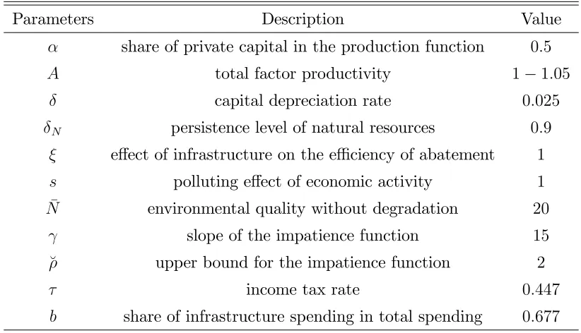
resort to numerical simulations, using the parameterization reported in Table A. The values of
the economic parameters are as in most dynamic general equilibrium calibration and estimation
studies.
The values used for the productivity of private capital in the production function, , and the
capital depreciation rate, , come from Economides and Philippopoulos (2008) and
Dioikitopou-los and Kalyvitis (2010). Following common practice, we use the TFP,A, as a scale parameter
to help us get plausible values for the growth rates. We set the values for the detrimental e¤ect
of consumption on the environment,s, and the exogenous e¤ectiveness of environmental policy,
, following Economides and Philippopoulos (2008), while for the regeneration rate of natural
resources, N, we use a value that is su¢ ciently high to ensure a non-negative growth rate for
the environmental stock. We employ a linear time preference function, (N) = (N) + ,
> 0, for computational tractability (see, e.g., Pittel, 2002; Dioikitopoulos and Kalyvitis,
2010), which is rich enough to obtain our main results. The chosen values for the lower bound,
, and slope, , help us calibrate values for in line with the literature. In particular, the
(1996), while those reported for the high-growth regime are in the range commonly employed
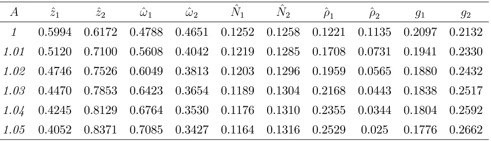
[image:17.612.70.548.144.282.2]in the growth literature.
Table 1. Technological Progress, Growth and the Environment
A z^1 z^2 !^1 !^2 N^1 N^2 ^1 ^2 g1 g2
1 0.5994 0.6172 0.4788 0.4651 0.1252 0.1258 0.1221 0.1135 0.2097 0.2132
1.01 0.5120 0.7100 0.5608 0.4042 0.1219 0.1285 0.1708 0.0731 0.1941 0.2330
1.02 0.4746 0.7526 0.6049 0.3813 0.1203 0.1296 0.1959 0.0565 0.1880 0.2432
1.03 0.4470 0.7853 0.6423 0.3654 0.1189 0.1304 0.2168 0.0443 0.1838 0.2517
1.04 0.4245 0.8129 0.6764 0.3530 0.1176 0.1310 0.2355 0.0344 0.1804 0.2592
1.05 0.4052 0.8371 0.7085 0.3427 0.1164 0.1316 0.2529 0.025 0.1776 0.2662
A higher value of A, representing technological progress in an economy, typically raises
output. In an economy characterized by a low level of environmental quality, and in turn less
patience and lower propensity to save, an increase in output raises consumption proportionately
more than private saving and causes more pollution and worsens environmental quality. A
slowly growing economy will also end up with a low tax base, and will have lower resources to
allocate to both infrastructure and abatement, so that the environmental quality deteriorates
further, raising the degree of impatience and giving rise to a further growth-reducing e¤ect.
Exactly the opposite happens to the high-growth equilibrium, which experiences less pollution,
better environmental quality, lower degree of impatience and higher growth. Table 1 provides
a numerical example to substantiate this theoretical result.
Result 1 An increase in TFP negatively a¤ects environmental quality and growth in
rela-tively poor economies and posirela-tively a¤ects environmental quality and growth in relarela-tively rich
economies.
4
Ramsey …scal policy
In this section we endogenize …scal policy, as summarized by the time paths of the two policy
instruments, 0 < < 1 and 0 < b 1, by solving for the Ramsey second-best problem
allocations, the Ramsey problem for the government is to pick the …scal policy that generates
the competitive equilibrium allocation with the highest value of this criterion.18
De…nition 2 A Ramsey Allocation is given under De…nition 1 when (i) the government chooses
the tax rate, , and the allocation of revenues to infrastructure and public abatement, b, in
order to maximize the welfare of the economy by taking into account the aggregate optimality
conditions of the competitive equilibrium, and (ii) the government budget constraints and the
feasibility and technological conditions are met.
In particular, the government seeks to maximize welfare in the economy subject to the
outcome of the decentralized equilibrium, summarized by (15)-(18). Due to the variable RTP,
Pontryagin’s maximum principle cannot be applied directly. To solve the problem within the
standard optimal control framework, we follow the procedure employed by Obstfeld (1990) and
introduce an additional ‘arti…cial’variable that accounts for the development of the
accumu-lated discount rate, (t) R0t (Nv)dv. Then, the objective of the government is to maximize
intertemporal utility:
maxUR =
Z 1
0
(vlnC+ (1 v) lnN) exp
Z t
0
(N)dv dt
constrained by the competitive equilibrium, (15)-(18), and the derivative of (t) with
respect to time, _ = ( ).
The Hamiltonian of the problem is given by:
RSB = [ logC+ (1 ) log(N)]e +
CC[a(1 )A
K Kg
a 1
(N)]
+ K (1 )AKaKg1 a C K + Kg b AK
aK1 a
g Kg
+ N (1 N)N (1 N)N
(1 b)
C Kg
+ (N)
18For second-best policies in models with environmental resources, see e.g Antoniou, Hatzipanayotou and
The …rst-order conditions of the Ramsey problem include the Euler equation, the growth
rates of private capital, public capital and environmental quality, the resource constraint, and
the optimality conditions with respect to C,Kg,K; N, , b, :
Ce + C "
Aa(1 ) K
Kg a 1
(N)
#
K N
(1 b) 1
Kg
= C (26)
CC Aa(1 ) (a 1)Ka 2Kg1 + K
"
A(1 ) K
Kg
a 1 #
+ KgAb
K Kg
a 1
= K
(27)
CC Aa(1 ) (1 )Ka 1Kg + K(1 ) (1 )A
K Kg
a
+ Kg b (1 )A
K Kg
a
+ N
(1 b)
C K2
g
= Kg (28)
(1 )
N e CC
0(N)
N(1 N) + 0(N) = N (29)
CC "
aA K Kg
a 1#
KAKaKg1 a+ KgAbK
aK1 a
g + N
(1 b) 2
C Kg
= 0 (30)
Kg AK
a
Kg1 a N
(1 b)2
C Kg
= 0 (31)
[ logC+ (1 ) logN]e = (32)
where C; K; Kg; N; are the dynamic multipliers associated with (26), (27), (28), (29).
Then, condition _ = ( ) and equations (26)-(32) characterize the dynamics of the Ramsey
problem. To obtain the long-run solution of the problem we de…ne the stationary variables:
! KC, z KgK, c ~CC, ~KK, g ~KgKg where ~i = e i. After some algebra the
long-run Ramsey equilibrium is given by:
+ ~chAa(1 ~)~za 1 N~ i ~ ~! ~N
(1 ~b)~!~z~= (A
~( ~N) = N~ + (34)
~
ca(1 ~) (a 1)Az~a 1+ ~ (1 ~)A z~a 1 + ~gA~b~ ~za= (A~b~~za )~ + ~( ~N)~ (35)
~
c Aa(1 ~) (1 ) ~za 1 + ~A(1 ~) (1 ) ~za 1
+ ~g h
A~b~ (1 ) ~za i+ ~N
(1 ~b)~!~z~= (A
~b~~za )~
g+ ~( ~N)~g (36)
~
c aAz~a 1 ~Az~a 1+ ~gA~bz~a+ ~N
~
!z~
(1 ~b)~2 = 0 (37)
(1 ) c~~0( ~N) ~N ~NN~(1 N) ~( ~N) NN~ = 0 (38)
A~g~~za ~N
~
!z~
(1 ~b)2~ = 0 (39)
A(a 1)(1 ~)~za 1 ~ (N) + ~! (40)
~
! =A(1 ~)~za 1 A~b~~za (41)
~
N =N [(1 ~)Az~a ~b~Az~a+1] (42)
Equations (33)-(42) describe a system of 10 equations with 10 unknowns, z~, ~b, ~, !~, N~,
~, ~g, ~N, ~, ~c. Due to the complexity of the system, we resort to numerical simulations.
We aim …rst, to examine the role of Ramsey government in equilibrium selection, and second,
to examine the e¤ect of an increase in technological progress (increase in A) on the patience
level, policy instruments, growth and the environment. We follow exactly the same numerical
parameter values used in the DCE, except for the endogenous policy instruments,~ and~b, that
are derived through the Ramsey objective.
Out of the good and bad equilibria (that existed under the DCE), the bad equilibrium is
eliminated under optimal …scal policy to yield a unique equilibrium with high growth and
envi-ronmental quality.19 This happens because the government chooses the aggregate endowments
19Note that for A = 1 and the endogenous taxes from the Ramsey problem, the DCE solution gives two
(that are taken as given in the DCE) to choose a consumption and saving path that puts the
economy in the high growth equilibrium, and then uses the policy instruments to attain the
[image:21.612.129.483.169.307.2]welfare-maximizing objective.
Table 2. Technological Progress, Ramsey Fiscal Policy and the Environment
A z~ ~b ~ !~ N~ ~ g~
1 0.6172 0.6773 0.4475 0.4651 0.1258 0.1135 0.2132
1.01 0.6122 0.6782 0.4495 0.4696 0.1257 0.1143 0.2160
1.02 0.6074 0.6790 0.4515 0.4741 0.1256 0.1152 0.2187
1.03 0.6026 0.6799 0.4534 0.4786 0.1256 0.1160 0.2215
1.04 0.5980 0.6808 0.4553 0.4831 0.1255 0.1169 0.2243
1.05 0.5933 0.6816 0.4573 0.4876 0.1254 0.1177 0.2271
Regarding changes in technology, our numerical results in Table 2 show that higher TFP
raises output and creates incentives for the utilitarian government to generate higher tax
rev-enues and allocate a higher proportion of its spending towards infrastructure. This results
in even higher growth, even if this comes at the cost of slightly lower environmental quality.
This outcome is in contrast to the dynamics of the DCE scenario where policy instruments are
exogenous. Intuitively, after an increase in TFP, government expenditures on infrastructure
become more e¤ective in raising output. In turn, the government has an incentive to increase
the allocation of revenues towards infrastructure so as to increase growth, and then to generate
a higher tax base to …nance expenditures for the environment. However, the consumption e¤ect
of higher growth outweighs that of higher abatement expenditures and causes a net increase in
pollution. Interestingly, in our numerical simulations, even though we used a higher weight on
environmental preferences vis-a-vis consumption, (1 v = 0:8), the net utility bene…t of raising
consumption is positive.
Result 2 The Ramsey government leads the economy to a unique equilibrium that
corre-sponds to the high-growth DCE regime. Under an increase in technology, government
realloca-tion of public revenues from environment to infrastructure has a positive e¤ect on growth while
5
Conclusion
The objective of this paper was to explore possible explanations about two stylized facts: (i)
across countries, advanced economies on average perform better in terms of growth and
envi-ronmental quality, while developing countries often stagnate with low growth and low
environ-mental quality; (ii) fast-growing economies could actually end up polluting the environment,
ex post, despite there being increases in TFP, which could have been utilised to …nance
pollu-tion abatement. We have studied an endogenous growth model of the environment, both for a
decentralized economy and for an economy with an optimizing (Ramsey) government. In our
set-up, the representative agent derived utility from private consumption and environmental
quality, and an important feature of the utility function was that the rate of time preference was
a decreasing function of the quality of the environment. Also, the environment was degraded
by pollution, which was a by-product of consumption, and was replenished by abatement
activ-ities undertaken by the government. Other than the environment, the government also spent
on infrastructure from the income taxes it generated, while balancing its budget. Externalities
in production were generated by public capital, and the services from infrastructure positively
a¤ected the e¢ ciency of abatement.
Our results for a decentralized economy highlight the existence of multiple equilibria. Here,
the good equilibrium is characterized by a higher growth rate driven by a higher
private-to-public capital ratio, higher marginal productivity of capital, lower propensity to consume
resulting in lower pollution, and higher environmental quality. This, in turn, implies a lower
degree of impatience, thus strengthening the growth channel and leading to ever-increasing
growth and better environmental quality at the same time. The bad equilibrium is characterized
by exactly the opposite e¤ects, pushing the economy in a downward spiral. Technological
progress in such an economy has adverse e¤ects on growth and the environment, in sharp
contrast to the favourable e¤ects of the same for the good equilibrium.
For the case of a Ramsey-government that chooses its policy instruments to maximize agents’
equi-librium that remains is a high-growth equiequi-librium. The response to higher TFP in this case is
for the government to spend a higher proportion of its revenue on infrastructure, which would
dynamically lead to a higher growth rate and utility levels in the long-run, even if these come
at the cost of a somewhat lower environmental quality, ex post. We hope that our …ndings will
provide valuable insights into the complex relationships that exist among governmental policy,
economic growth and the environment.
References
[1] Andreoni J. and Levinson, A. (2001). The simple analytics of the environmental Kuznets curve. Journal of Public Economics, 80, 269-286.
[2] Antoniou, F., Hatzipanayotou, P., and Koundouri, P. (2012). Second best environmental policies under uncertainty. Southern Economic Journal, 78(3), 1019-1040.
[3] Ayong Le Kama, A. and Schubert, K. (2007). A note on the consequences of an endogenous discounting depending on the environmental quality. Macroeconomic Dynamics, 11, 272-289.
[4] Barman, T. R., and Gupta, M. R. (2010). Public expenditure, environment, and economic growth. Journal of Public Economic Theory, 12, 1109-1134.
[5] Barro, R. J. (1990). Government spending in a simple model of endogenous growth. Journal of Political Economy, 98, 103-125.
[6] Beckerman, W. (1992). Economic growth and the environment: Whose growth? Whose environment? World Development, 20, 481–496.
[7] Benarroch, M. and Weder, R. (2006). Intra-industry trade in intermediate products, pol-lution and internationally increasing returns. Journal of Environmental Economics and Management, 52, 675–689.
[8] Bertinelli, L., Strobl, E. and Zou, B. (2008). Economic development and environmental quality: a reassessment in light of nature’s self-regeneration capacity. Ecological Economics, 66, 371-378.
[9] Bovenberg, L. and Smulders, S. (1995). Environmental quality and pollution-augmenting technological change in a two-setor endogenous growth model. Journal of Public Economics, 57, 369-391.
[10] Bretschger L. and Smulders, S. (2006). Sustainable resource use and economic dynamics. Environmental and Resource Economics, 33, 771-1054.
[12] Cassou, S. P. and Hamilton, S. F. (2004). The transition from dirty to clean industries: Optimal …scal policy and the environmental Kuznets curve. Journal of Environmental Economics and Management, 48, 1050-1077.
[13] Chavas, J-P. (2004). On impatience, economic growth and the environmental Kuznets curve: A dynamic analysis of resource management. Environmental and Resource Eco-nomics, 28, 123-152.
[14] Chu, H., Lai, C-C., and Liao, C-H. (2015). A note on environment-dependent time prefer-ences, Macroeconomics Dynamics, 1-16, forthcoming.
[15] Das, M. (2003). Optimal growth with decreasing marginal impatience. Journal of Economic Dynamics and Control, 27, 1881-1898.
[16] De Bruyn, S. M. and van den Bergh, J. C. J. M. & Opschoor, J. B. (1998). Economic growth and emissions: reconsidering the empirical basis of environmental Kuznets curves, Ecological Economics, 25, 161-175.
[17] Dioikitopoulos, E. V. and Kalyvitis, S. (2010). Endogenous time preference and public policy: Growth and …scal implications. Macroeconomics Dynamics, 14, 243-257.
[18] Economides, G. and Philippopoulos, A. (2008). Growth enhancing policy is the means to sustain the environment. Review of Economic Dynamics, 11, 207-219.
[19] Egli H. and Steger, T.M. (2007). A dynamic model of the environmental Kuznets curve: Turning point and public policy. Environmental and Resource Economics, 36, 15-34.
[20] Elbasha, E. H. and Roe, T. L. (1996). On endogenous growth: The implications of environ-mental externalities. Journal of Environenviron-mental Economics and Management, 31, 240-268.
[21] Freeman, M. and Groom, B. and Panopoulou, E. and Pantelidis, T. (2015) Declining dis-count rates and the Fisher e¤ect: In‡ated past, disdis-counted future? Journal of Environmetal Economics and Management, forthcoming.
[22] Futagami, K., Morita, Y. and Shibata (1993), A. Dynamic analysis of an endogenous growth model with public capital. Scandinavian Journal of Economics, 95, 607-625.
[23] Gradus, R. and Smulders, S. (1993). The trade-o¤ between environmental care and long-term growth: Pollution in three prototype growth models. Journal of Economics, 58, 25-51.
[24] Greiner, A. (2005). Fiscal policy in an endogeneous growth model with public capital and pollution. Japanese Economic Review, 56, 67-84.
[25] Grossman, G. M. and Krueger, A. B. (1995). Economic growth and the environment. Quarterly Journal of Economics, 110, 353-377.
[26] Gupta, M.R. and Barman, T. R. (2009). Fiscal policies, environmental pollution and economc growth. Economic Modelling, 26, 1018-1028.
[28] Hatzipanayotou, P., Michael, M. S., and Lahiri, S. (2003). Environmental policy reform in a small open economy with public and private abatement, in Environmental Policy in an International Perspective, edited by L. Marsiliani, M. Rauscher and C. withagen, Kluwer, London.
[29] Hepburn, C. & Koundouri, P. & Panopoulou, E. & Pantelidis, T. 2009. Social discounting under uncertainty: A cross-country comparison, Journal of Environmental Economics and Management, Elsevier, vol. 57(2), pages 140-150, March.
[30] Hilton, F. G. H. and Levinson, A. (1998). Factoring the environmental Kuznets curve: evidence from automotive lead emissions. Journal of Environmental Economics and Man-agement, 35, 126-141.
[31] Holtz-Eakin, D. and Selden, T. (1995). Stoking the …res? CO2 emissions and economic
growth. Journal of Public Economics, 57, 85-101.
[32] Howarth, R. B. (1996). Discount rates and sustainable development. Ecological Modelling, 92, 263-270.
[33] Itaya, J.-i. (2008). Can environmental taxation stimulate growth? The role of indetermi-nacy in endogenous growth models with environmental externalities. Journal of Economic Dynamics and Control, 32, 1156-1180.
[34] John, A. and Pecchenino, R. (1994). An overlapping generations model of growth and the environment. Economic Journal, 104, 1393-1410.
[35] Jones, L. and Manuelli, R. (2001). Endogenous policy choice: The case of pollution and growth. Review of Economic Dynamics, 4, 369-405.
[36] Jouvet, P-A, Pestieau, P. and Ponthiere, G. (2010). Longevity and environmental quality in an OLG model. Journal of Economics, 100, 191-216.
[37] Kahn, M.E. (1998). A household level environmental Kuznets curve. Economics Letters, 59, 269-273.
[38] Liddle, B. (2001). Free trade and the environment-development system. Ecological Eco-nomics, 39, 21-36.
[39] Ligthart, J. E. and Ploeg, F. v. (1994). Pollution, the cost of public funds and endogenous growth. Economics Letters, 46, 339-349.
[40] List, J. A. and Gallet, C. A., (1999). The environmental Kuznets curve: does one size …t all? Ecological Economics, 31, 409-423.
[41] Managi, S. (2006). Are there increasing returns to pollution abatement? Empirical analyt-ics of the environmental Kuznets curve in pesticides. Ecological Economanalyt-ics, 58, 617-636.
[43] Michael, M. S., Lahiri, S., and Hatzipanayotou, P. (2015). Piecemeal reform of domestic indirect taxes toward uniformity in the presence of pollution: with and without a revenue constraint. Journal of Public Economic Theory, 17, 174-195.
[44] Millimet, D. L., List, J. A. and Stengos, T. (2003). The environmental Kuznets curve: Real progress or misspeci…ed models? The Review of Economics and Statistics, 85, 1038–1047.
[45] Mohtadi, H. (1996). Environment, growth and optimal policy design. Journal of Public Economics, 63, 119-140.
[46] Obstfeld, M. (1990). Intertermporal dependence, impatience, and dynamics. Journal of Monetary Economics, 26, 45-75.
[47] Pautrel, X. (2009). Pollution and life expectancy: How environmental policy can promote growth. Ecological Economics, 68, 1040-1051.
[48] Pautrel, X. (2012). Pollution, private investment in healthcare, and environmental policy. Scandinavian Journal of Economics, 114, 334-357.
[49] Perez, R. and Ruiz, J. (2007). Global and local indeterminacy and optimal environmental public policies in an economy with public abatement activities. Economic Modelling, 24, 431-452.
[50] Pittel, K. (2002). Sustainability and Endogenous Growth. Cheltenham, UK: Edward Elgar.
[51] Quaas, M. F. (2007). Pollution-reducing infrastructure and urban environmental policy. Environment and Development Economics, 12, 213-234.
[52] Schumacher, I. (2009). Endogenous discounting via wealth, twin-peaks and the role of technology. Economics Letters, 103, 78-80.
[53] Selden, T.M. and Song, D. (1994). Environmental quality and development: Is there a Kuznets curve for air pollution emissions? Journal of Environmental Economics and Man-agement, 27, 147-162.
[54] Selden, T.M. and Song, D. (1995). Neoclassical growth, the J curve for abatement, and the inverted U curve for pollution. Journal of Environmental Economics and Management, 29, 162-168.
[55] Smulders, S. and Gradus, R. (1996). Pollution abatement and Long-Term Growth. Euro-pean Journal of Political Economy, 12, 505-532.
[56] Stern, D. I., Common, M. S. and Barbier, E. B. (1996). Economic growth and environmen-tal degradation: The environmenenvironmen-tal Kuznets curve and sustainable development. World Development, 24, 1151-1160.
[57] Suri, V. and Chapman, D. (1998). Economic growth, trade and energy: implications for the environmental Kuznets curve. Ecological Economics, 25, 195-208.
[59] Turnovsky, S. J. (2000). Methods of Macroeconomic Dynamics. MIT Press.
[60] Varvarigos, D. (2014). Endogenous longevity and the joint dynamics of pollution and cap-ital accumulation. Environment and Development Economics, 19, 393-416.
[61] Vella, E., Dioikitopoulos, E. V. and Kalyvitis, S. (2015). Green spending reforms, growth and welfare with endogenous subjective discounting. Macroeconomic Dynamics, 19, 1240-1260.
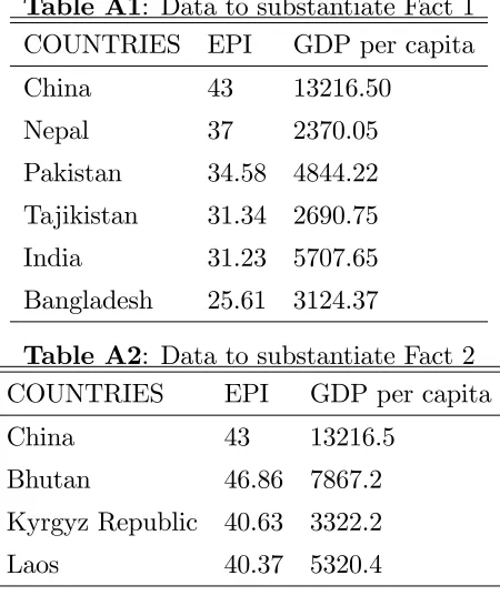
Appendix A: Data in support of Facts 1 and 2
Considering China in relation to some of its neighbouring countries in geographic terms,
we can observe two trends: …rst, that the EPI and GDP per capita of China are both higher
(sometimes, considerably more so) than countries like Nepal, Pakistan, Tajikistan, India and
Bangladesh; and second, that while China’s EPI is very similar to some other neighbouring
countries (like Bhutan, Kyrgyz Republic and Laos), its GDP per capita is much higher than
those countries. This information is reported in Tables A1 and A2 below, respectively. Table
A1 shows that in relation to China, the other countries perform relatively poorly in terms of
the environment index as well as the income per capita measure (in particular, Tajikistan and
Bangladesh fare rather badly in terms of environment and income performance), which is in
conformity with Fact 1, suggesting the presence of multiple equilibria. On the other hand, Table
A2 shows that China has almost double the income per head of Bhutan, but has a lower EPI
value; comparing China with Laos and Kyrgyz Republic, we …nd that China has about three
times more income per head than those two countries but only slightly better environmental
quality, which suggests Fact 2, that economic policies in fast-growing countries may not be
[image:28.612.194.419.469.742.2]environmentally friendly relative to some slower-growing nations.
Table A1: Data to substantiate Fact 1 COUNTRIES EPI GDP per capita
China 43 13216.50
Nepal 37 2370.05 Pakistan 34.58 4844.22
Tajikistan 31.34 2690.75
[image:28.612.200.417.476.616.2]India 31.23 5707.65 Bangladesh 25.61 3124.37
Table A2: Data to substantiate Fact 2 COUNTRIES EPI GDP per capita
China 43 13216.5
Bhutan 46.86 7867.2 Kyrgyz Republic 40.63 3322.2
Appendix B: Proof of Proposition 1
Let us …rst investigate the conditions for a well-de…ned equilibrium in the long run. In order
for !^(^z) > 0 to hold, we must have z <^ 1b from (23). Combining all the above we get the
following for the domain of z^: b
1
a
<z <^ 1b .
The method will be to separate function (^z) Ab z^a+Aa(1 )^za 1 (N [(1
)Az^a b Az^a+1]) in two functions and …nd their intersection to solve it. We de…ne (^z)
Aa(1 )^za 1 Ab z^a and (^z) (N [(1 )Az^a b Az^a+1]). Both (^z) and (^z)are
continuous in z^. In order for!^(^z)>0to hold we must have z <^ 1v .
Equation (^z) has the following properties:
1. limz^!0 (^z) = +1 , limz^!1b (^z) =Aa(1 )(
1
b )
a 1 Ab (1
b )
a.
2. @@(^z^z) <0, @2@z^(^2z) >0:
From the properties of (^z)is follows that it is a strictly decreasing and convex function in
its domain, starts from+1 and ends atAa(1 )(1b )a 1 Ab (1
b )
a.
Equation (^z) has the following properties:
1. limz^!0 (^z) = (N) = , limz^!1b (^z) = (0) = .
2. @@(^z^z) = 0(:) [aA(1 )^za 1 b (1 +a)^za]. We have @ (^z)
@z^ >0 fora(1 )^z
a 1 b(1 +
a) ^za > 0 =) z <^ ba(1+(1 a)) and @@(^z^z) < 0 for z >^ ba(1+(1 a)). Thus, (^z) has a maximum at
^
z = ba(1+(1 a)).
From the properties of (^z) it follows that it is an inverse U-shaped curve starting from
and ending at .
Assuming equilibrium existence, from the properties of (^z) and (^z) it follows that there
exist one or two positive balanced growth rates. For low values of z^, since+1> we get that
(^z)lies above (^z). Also, for the upper bound value ofz^, (^z) = Aa(1 )(1b )a 1 Ab (1
b )
a
and (^z) = . Since both functions are continuous, ifAa(1 )(1b )a 1 Ab (1b )a< , which
means that (^z)starts above and ends below (^z)implying that (^z)will cross (^z)once and
there will exist a unique balanced growth rate. Thus, Aa(1 )(1
b )
a 1 Ab (1
b )
a< is a
If Aa(1 )(1
b )
a 1 Ab (1
b )
a then there can exist two balanced growth rates
because (^z) is an inverse U-shaped curve, while (^z) strictly monotone and decreasing, so
(^z)can cross (^z)at most two times. Thus,Aa(1 )(1b )a 1 Ab (1
b )
a is a necessary
parametric condition for multiplicity.
Ranking of Equilibria: In the case of multiple balanced growth rates (^z)and (^z)intersect
twice, for z^1 and z^2. Let those two balanced growth rates ranked as z^1 > z^2. To …nd the
corresponding ranking of !^1 and !^2 we solve !^ in the steady-state, and we take the derivative
with respect to z^, @@!^^z = (a 1)(1 )Az^a 2 abA z^a 1 < 0. Thus, !^ is a strictly decreasing
function of z^, so z^1 >z^2 =)!^1 < !^2. To …nd the ranking of g1 and g2 we take the derivative
of g with respect to z^, @g@z^ = b az^a 1 > 0. Thus, g is an increasing function of z^, so z^ 1 >
^
z2 =) g1 > g2. The ranking for the rate of time preference, (^z !^(^z)) = (^z), which is a
non-monotonic function of z^, comes from the analysis above. As (^z) lies above (^z) and is
monotonically decreasing, it cannot cross twice (^z) in its increasing part. Then, z^1 >z^2 =)
(^z1)< (^z2) =) (^z1)< (^z2) =) 1 < 2. So, in case of two balanced growth rates with
high growth, g1, and low growth,g2, the endogenous variables are ranked as 1 < 2, !^1 <!^2,
^
Appendix C: Numerical analysis
Table A3. Values for parameters and exogenous policy instruments
Parameters Description Value
share of private capital in the production function 0:5
A total factor productivity 1 1:05
capital depreciation rate 0:025
N persistence level of natural resources 0:9
e¤ect of infrastructure on the e¢ ciency of abatement 1
s polluting e¤ect of economic activity 1
N environmental quality without degradation 20
slope of the impatience function 15
upper bound for the impatience function 2
income tax rate 0:447