Bookmarking Systems
.
White Rose Research Online URL for this paper:
http://eprints.whiterose.ac.uk/108764/
Version: Accepted Version
Article:
Doerfel, S., Jäschke, R. and Stumme, G. (2016) The Role of Cores in Recommender
Benchmarking for Social Bookmarking Systems. ACM Transactions on Intelligent Systems
and Technology, 7 (3). 40. 40:1-40:33. ISSN 2157-6904
https://doi.org/10.1145/2700485
eprints@whiterose.ac.uk
Reuse
Unless indicated otherwise, fulltext items are protected by copyright with all rights reserved. The copyright exception in section 29 of the Copyright, Designs and Patents Act 1988 allows the making of a single copy solely for the purpose of non-commercial research or private study within the limits of fair dealing. The publisher or other rights-holder may allow further reproduction and re-use of this version - refer to the White Rose Research Online record for this item. Where records identify the publisher as the copyright holder, users can verify any specific terms of use on the publisher’s website.
Takedown
If you consider content in White Rose Research Online to be in breach of UK law, please notify us by
The Role of Cores in Recommender Benchmarking for Social
Bookmarking Systems
STEPHAN DOERFEL, KDE Group, ITeG, University of Kassel, Germany
ROBERT J ¨ASCHKE, L3S Research Center, Hannover, Germany
GERD STUMME, KDE Group, ITeG, University of Kassel, Germany and L3S
Social bookmarking systems have established themselves as an important part in today’s web. In such sys-tems,tag recommender systemssupport users during the posting of a resource by suggesting suitable tags. Tag recommender algorithms have often been evaluated in offline benchmarking experiments. Yet, the par-ticular setup of such experiments has rarely been analyzed. In parpar-ticular, since the recommendation quality usually suffers from difficulties like the sparsity of the data or the cold start problem for new resources or users, datasets have often been pruned to so-calledcores(specific subsets of the original datasets) – however without much consideration of the implications on the benchmarking results.
In this paper, we generalize the notion of a core by introducing the new notion of aset-core– which is independent of any graph structure – to overcome a structural drawback in the previous constructions of cores on tagging data. We show that problems caused by some types of cores can be eliminated using set-cores. Further, we present a thorough analysis of tag recommender benchmarking setups using set-cores. To that end, we conduct a large-scale experiment on four real-world datasets in which we analyze the influence of different cores on the evaluation of recommendation algorithms. We can show that the results of the comparison of different recommendation approaches depends on the selection of core type and level. For the benchmarking of tag recommender algorithms, our results suggest that the evaluation must be set up more carefully and should not be based on one arbitrarily chosen core type and level.
CCS Concepts:•General and reference→Evaluation;Experimentation; Measurement;•Information systems→Recommender systems;•Human-centered computing→Social recommendation; Social tagging; Social tagging systems;
Additional Key Words and Phrases: Recommender; Core; Benchmarking; Graph; Evaluation; Preprocessing
ACM Reference Format:
Stephan Doerfel, Robert J ¨aschke and Gerd Stumme, 2013. The Role of Cores in Recommender Benchmark-ing for Social BookmarkBenchmark-ing Systems.ACM Trans. Intell. Syst. Technol.V, N, Article XXXX (July 2015), 33 pages.
DOI:http://dx.doi.org/10.1145/2700485
1. INTRODUCTION
Recommender systems have become a vital part of the social web, where they assist users in their content selection by pointing to personalized sets of resources. Such sys-tems often have to deal with sparse data since only little or nothing is known about many users or items. Alongside work that specifically tackles this task, in the
eval-Part of this work was funded by the DFG in the project “Info 2.0 – Informationelle Selbstbestimmung im Web 2.0”.
Author’s addresses: S. Doerfel and G. Stumme, Knowledge & Data Engineering Group (KDE) at the Interdis-ciplinary Research Center for Information System Design (ITeG) at the University of Kassel, Wilhelmsh¨oher Allee 73, 34121 Kassel, Germany; R. J ¨aschke, L3S Research Center, Appelstraße 4, 30167 Hannover, Ger-many;
Permission to make digital or hard copies of all or part of this work for personal or classroom use is granted without fee provided that copies are not made or distributed for profit or commercial advantage and that copies bear this notice and the full citation on the first page. Copyrights for components of this work owned by others than the author(s) must be honored. Abstracting with credit is permitted. To copy otherwise, or republish, to post on servers or to redistribute to lists, requires prior specific permission and/or a fee. Request permissions from permissions@acm.org.
c
2015 Copyright held by the owner/author(s). Publication rights licensed to ACM. 2157-6904/2015/07-ARTXXXX $15.00
uation of recommender algorithms it is common to focus on a denser subset of the data [Sarwar et al. 2001] that provides enough information to produce helpful recom-mendations. For data that can be modeled as a graph, a commonly used technique are
generalized cores[Batagelj and M. Zaverˇsnik 2002] which comprise a dense subgraph
in which every vertex fulfills a specific constraint, e.g., the degree of each node is above a certain threshold, the so-called core-level. However, the influence of these cores on the evaluation of recommendation algorithms has not been analyzed so far.
In this paper, we investigate cores that have been used in the evaluation of tag
recommender systems. Tag recommenders are useful in social bookmarking systems
where users post resources (like bookmarks for websites, scientific publications, videos,
or photos) and assign arbitrary keywords (tags) to them. During the posting process
a recommender system typically suggests appropriate tags for annotation. The tag recommendation task is thus to find suitable tags for a given user and resource.
Previously, tag recommender algorithms have often been evaluated on a special gen-eralized core of the raw dataset. Although the use of cores is quite common in tag rec-ommender benchmarking (cf. Section 3), it has rarely been analyzed how the choice of
— core type(i.e., the method to construct the core as a subset of the original dataset;
we will recall and introduce various core types in Section 2),
— core level(i.e., the threshold that is imposed on some property of each data point to
construct the subset; see Section 2, Definitions 2.1 and 2.2),
or simply the process of constructing cores influences the results of such experiments. In fact, the choice of these setup parameters has been rather diverse in previous tag recommender benchmarking experiments (see the related work in Section 3 for details and for examples from the literature). Especially, the core level is often set ad-hoc – without a motivation for the particular choice – to such values as 2, 5, or even 100, or to dataset-dependent thresholds. In our experiments in Section 4 we show on real world datasets, that the choice of core type and core level indeed has an impact on a benchmarking’s ranking of recommender algorithms. In fact, different experiments on different setups can lead to contradictory results. Thus, much like the choice of the evaluation metric or the sampling of training and test data, the core type and level are important aspects of an experimental setup. During the evaluation of different recommendation algorithms or during parameter optimization of such algorithms, it is therefore worthwhile to experiment with several cores and also to use the raw datasets (the unrestricted datasets). Moreover, the choice of particular core-levels should be motivated by the use-case and comparisons of results from different experiments must consider the different core setups in each experiment.
While the previously used cores indeed yield denser graphs, they also come with the unpleasant property ofdiminishing posts, i.e., a post of the raw dataset – consisting of a user, a resource, and several tags – might still occur in the core but with fewer tags. Thus, the core construction not only reduces the number of posts in the dataset, but modifies the posts themselves. For such “diminished” posts the recommendation prob-lem becomes more difficult as recommended tags will not be considered good recom-mendations even when they actually belong to the original post but have been removed from that post by the core construction.
We show that cores of real-world datasets indeed contain many such diminished posts and that different recommender algorithms often yield lower quality scores on such posts than on those that still remain intact with all their tags in the core.
To overcome this structural problem we first generalize the notion of generalized
cores [Batagelj and M. Zaverˇsnik 2002] even further to yieldset-cores(Section 2). In
that set-cores have similar properties as generalized cores, describe a construction al-gorithm, and prove its correctness. We then construct a new kind of core – a set-core – for social bookmarking systems which guarantees to leave all remaining posts intact (undiminished).
In Section 3 we discuss how the experimental setup and evaluation using cores has been handled in previous work on tag recommendations. We then choose a common setup and describe in Section 4 several experiments on four publicly available real-world datasets to investigate the influence of cores on the results of recommender systems benchmarking. We discuss the results of these experiments in Section 5 where we show how different cores can lead to contradictory results in the comparison of algorithms. We also point to a peculiarity that arises from using any type of core in that setup. To summarize, the contributions of this paper are fourfold:
— We generalize the notion of generalized cores toset-coresand introduce new cores
for tagging data of social bookmarking systems to eliminate the particular anomaly of diminished posts in previously used cores.
— We present a thorough investigation of the influence of cores on the results of tag recommender benchmarking experiments and confirm that different choices of core type and level can indeed yield different results.
— We discuss potential pitfalls of the use of cores in recommender evaluation.
— We provide recommendations for the use of cores in future tag recommender bench-marking experiments.
2. CORES OF GRAPHS AND SETS
Before we discuss the influence of cores within the benchmarking framework for tag recommendations, we deal with the notion of a core itself. In social bookmarking sys-tems (often also calledtagging systems, see Section 2.3 for a formal definition of their data structure), the cores that have been used so far have the unpleasant property of diminishing posts by removing tags. In this section we present a solution to that prob-lem by introducing post-set-cores. To accomplish that we first recall the notion of gen-eralized cores of a graph and then extend it to arbitrary sets by introducing set-cores (Section 2.1). We present examples in Section 2.2 that illustrate different set cores and that demonstrate some advantages of set cores. We then discuss cores for tagging data in Section 2.3 where we recall the definitions of cores previously used for the evalua-tion of tag recommenders and we introduce a new core construcevalua-tion using set-cores to overcome the issue of diminished posts.
Notation. In the remainder of the paper we make use of the following usual notation:
— A graph G = (V, E)is given as a set V of verticestogether with a setE of
(undi-rected)edges. Hereby each edge connects two – or more (in the case of hypergraphs)
– vertices.
— E|Cdenotes the restriction of the setEto a subsetC⊆V, i.e., to the edges fromE
between vertices fromC.
— WithP(S)we denote thepower setof a given setS.
Batagelj and Zaverˇsnik presented the notion ofp-cores in [Batagelj and M. Zaverˇsnik 2002], which by itself is a generalization of the original cores introduced in [Seidman
1983]. In the sequel, we refer to their construction asgraph-p-coresto better
distin-guish them from the new notion ofset-P-coreswhich we introduce later in this section. The idea of graph-p-cores is to restrict a given graph by removing all nodes for which a particular quantityp(e.g., the vertex degree) does not exceed a given thresholdlcalled
thecore level. The graph-p-core is then the largest possible subgraph such that all its
Definition2.1 (Graph-p-Core [Batagelj and M. Zaverˇsnik 2002]). LetG= (V, E)be a graph,l∈R, andpa vertex property function onG, i.e.,p:V ×P(V)→R: (v, W)7→ p(v, W). A subgraphH = (C, E|C)induced by the subset of verticesC ⊆V is called a
graph-p-core at levell, iffl≤p(v, C), for allv∈CandH is a maximum subgraph with
this property. A core of Gwith a maximum levell such that it is not empty is called
themain coreofG.
An example for a property functionpis the vertex degree in each subgraph – in fact,
the original core definition of Seidman [Seidman 1983] uses just that function instead of an arbitrary functionp.
The functionpis calledmonotoneif and only if it fulfills
W1⊆W2⊆V =⇒ ∀v∈W1:p(v, W1)≤p(v, W2).
[Batagelj and M. Zaverˇsnik 2002] prove that for every monotone vertex property func-tionpa graph-p-core is uniquely determined at each levelland that it can be computed by iteratively removing verticesvfrom the vertex setW(starting withW :=V) that do not fulfill l≤p(v, W). The monotonicity assumption is a mild requirement, as typical vertex property functions (like the degree) naturally fulfill it.
Note, that in Definition 2.1, the value p(v, W)of the function pis dependent both
on the vertex v and on the vertices W of the subgraph that it is evaluated on. For
example, the degree of a vertex in a subgraph ofGcan be smaller than its degree inG. Alternatively, the functionpin Definition 2.1 can be replaced by a set of functions
{pW:W →R|(W, E|W)is a subgraph ofG}.
A drawback of Definition 2.1 is that it is not possible to model simultaneous restric-tions of several properties (e.g., that a vertex has at least in-degreeland at least
out-degreem). This can be desirable, for example, when vertices are entities in a tagging
system and we want to require that each user has at least l posts, each resource
oc-curs in at least mposts, and each tag has been used at leastntimes. For the case of
two thresholds on a bipartite graph a solution was given in [Ahmed et al. 2007] by the introduction of graph-(p, q)-cores. Theset-P-core, which we introduce next, allows us to enforce different thresholds in a more general way by using an arbitrary partially ordered set1as a range instead of only the real numbers.
Another drawback of Definition 2.1 is the dependence on a graph structure. While this is quite universal already – as almost any kind of data can be modeled as a graph – it is not always particularly intuitive to construct a graph such that a graph-p-core can be constructed. In contrast, set-P-cores can be constructed on arbitrary sets.
2.1. Generalization
In the following, we present the definition of aset-P-core, prove its uniqueness and
de-scribe a construction. A set-P-core can be constructed on some arbitrary setS where
for each element ofSsome property can be measured. Again, a thresholdlis imposed
to restrict the set to such elements where that property is above the threshold. In con-trast to graph-p-cores, the levellmust not necessarily be a real number but must sim-ply belong to some partially ordered set L(like, for example, the spaceRn). Thus the properties are also no longer required to yield a single number, allowing to enforce mul-tiple property restrictions simultaneously. Given a setS, the set-P-core is the largest
subset, such that for each element ofS the chosen property functionsP yield a value
that is larger than a fix levell. This is stated more formally in the next definition:
Definition2.2 (Set-P-Core). LetSbe a set,La partially ordered set with the order relation ≤, l ∈ L, and P a set of property functions pS˜: ˜S → L with s 7→ pS˜(s) for each S˜ ⊆ S. A subsetC of S is said tohave the l-property w.r.t.P, if it satisfies the conditionl≤pC(c)for allc∈C. The subsetCis calledset-P-core at levellofS, iff it is
a maximum subset ofSwith thel-property.
We simply say that a subset of S has the l-property, if the choice ofP is clear from
the context. Note, that in contrast to the generalized graph-p-cores in [Batagelj and
M. Zaverˇsnik 2002], Definition 2.2 does neither require any kind of graph structure, nor a linearly ordered set (like the real numbers for graph-p-cores). For two elements aandbof the partially ordered setL, we denote bya6≤bthatais not smaller than or equal tob, i.e., that eitherais larger thanbor thataandbare incomparable.
It is easy to see that graph-p-cores are special set-P-cores: In the notions of
Defi-nitions 2.1 and 2.2, we set S := V (the vertex set of G), L := R and use the set of
p-functions asP such that p˜S(s) :=p(s, E|S˜). A trivial observation is that the empty set∅ ⊆Shas thel-property w.r.t.P for anyPandl∈Land thus any setShas at least one subset with thel-property.
Similar to graph-p-cores, the unique existence of the set-P-core is guaranteed as
long as the property functions inP satisfy a mild monotonicity requirement: in each
subset of the original set, for each element, the property measured by the according
map inP is lower than or equal to the according value measured in the original set.
Furthermore, set-P-cores are nested in the sense that increasing the level l yields a
smaller core. These properties are formalized and proven in the following theorem:
THEOREM 2.3. Given S, L and P as in Definition 2.2. If the functions inP are monotone in the sense that
˜
S1⊆S2˜ ⊆S=⇒ ∀s∈S1˜ :pS˜1(s)≤pS˜2(s)
holds, then forl, l1, l2∈Lhold:
(1) The union of subsets ofSwith thel-property has thel-property.
(2) There exists exactly one set-P-core atl.
(3) The set-P-cores are nested, i.e., ifl1≤l2, then the set-P-core atl2is contained in the
set-P-core atl1.
PROOF. We start with the first property: Let I be an index set andS˜i (i ∈ I)be subsets ofSwith thel-property andU their union. Fors∈U, there is somei∈Isuch that s ∈ S˜i. By monotonicity of P we havel ≤ pS˜i(s) ≤ pU(s)and thus U has thel -property. The second property follows directly from the first, with the set-P-core being the union of all subsets ofShaving thel-property (and thus obviously being maximal). For the third property, letC1 andC2 be the respective set-P-cores at l1and l2. Then l1≤l2≤pC2(s)≤p(C1∪C2)(s). Thus(C1∪C2)has thel1property, and by the maximality ofC1as core at levell1followsC1= (C1∪C2)and thusC2⊆C1.
We have now established a generalized notion of cores and can reuse the simple con-struction algorithm from [Batagelj and Zaverˇsnik 2011] for such a set-P-core, given a finite setS (see Algorithm 1). The set-P-core can always be constructed simply by
re-moving one element violating the l-property after another until the remaining set of
removal) and thus be no longer larger than the thresholdl. We prove the applicability of Algorithm 1 in the following theorem:
ALGORITHM 1:Naive set-P-core construction Input: DatasetS, levell, monotone set of functionsP. Output: The set-P-coreCofSat levell.
C:=S;
while∃s∈Csuch thatl6≤pC(s)do C:=C\ {s};
end
THEOREM 2.4. GivenS,L,l ∈ L, andP as in Definition 2.2 withP being a set of
monotone functions. IfSis finite, then Algorithm 1 returns the set-P-core atlofS.
PROOF. Let D be the algorithm’s result and letC be the set-P-core ofS atl. The
unique existence ofC is already guaranteed by Theorem 2.3. From the algorithm it is
clear thatDhas thel-property and is therefore a subset ofC. Let furthers1, s2, . . . , sn be the elements ofS\Din the order of their deletion by the algorithm. AssumeD⊂C. Then we can select an index iwith1 ≤i ≤nsuch that for allj with1 ≤j < i,sj is inS\C butsiis inC. We setS˜i :=S\ {s1, s2, . . . , si−1} and yieldl 6≤pS˜i(si), sincesi was removed in theith step of the algorithm. From the selection of ifollows C ⊆ S˜i and thus by monotonicity ofP we havepC(si)≤pS˜i(si)and thereforel 6≤pC(si). This is a contradiction to thel-property ofC. We have thus establishedD=Cand conclude that the algorithm’s result is the set-P-core atlofS.
2.2. Examples
Our generalization allows us to transfer the concept of a core to arbitrary algebraic structures without constructing graphs. Although it is almost always possible to model a given dataset as a graph, it is not always convenient to impose a graph model. It is especially unpleasant when data is already modeled as a graph (like in the case of social bookmarking systems in the next section) but the graph does not allow the construction of a core in the desired way and thus a new graph would have to be introduced to support it. With set-cores, this is no longer an issue.
Before we leverage set-cores to construct cores for tagging data in the next section, we discuss a very simple example where data does not have to be modeled as a graph: a core that could be used in the evaluation of item recommendation algorithms. Let
U be a set of users and I a set of items. Further, let S ⊆ U ×I be the (user, item)
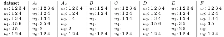
co-occurrences (i.e., the relation denoting which items a user likes). Such a setting is demonstrated with a toy example in the first column of Table I, where six users co-occur with (e.g., have expressed interest or have bought) six items in 18 (user, item) co-occurrences.
Now, letP be a set of mapsp˜S (for everyS˜⊆S) with
pS˜: ˜S→N: (u, i)7→max
{j ∈I|(u, j)∈S˜} ,
{v∈U |(v, i)∈S˜}
. (1)
For a given levell∈N, the set-P-core atlthen contains all (user, item) co-occurrences
from S such that each user occurs with at least l items or each item occurs with at
least lusers. Thus, at least one entity of each user-item-pair is frequent in the data-set. In the toy example in Table I, for each (user, item) co-occurrence the maximum of
Table I. A toy example for different cores in a user-item co-occurrence setting. The set U contains six users u1, u2, . . . , u6and the setIcontains six items1,2, . . . ,6. The first column shows the full dataset of users together
with their co-occurring items. Each further columnA1, A2, B, . . . , F shows a different restriction of that dataset.
The functions to create these subsets are described in Section 2.2.
dataset A1 A2 B C D E F
u1: 1 2 3 4 u1: 1 2 3 4 u1: 1 2 3 4 u1: 1 2 4 u1: 1 2 3 4 u1: 1 2 3 4 u1: 1 2 3 4 u1: 1 2 3 4 u2: 1 2 4 u2: 1 2 4 u2: 1 2 4 u2: 1 2 4 u2: 1 2 4 u2: 1 2 4 u2: 1 2 4 u2: 1 2 4 u3: 1 3 4 u3: 1 3 4 u3: 1 4 u3: u3: 1 3 4 u3: 1 3 4 u3: 1 3 4 u3: 1 3 4 u4: 3 5 6 u4: 3 5 6 u4: u4: u4: u4: 3 5 6 u4: 3 5 u4: 3 5
u5: 2 5 u5: 2 u5: 2 u5: u5: u5: u5: 2 5 u5:
u6: 1 2 4 u6: 1 2 4 u6: 1 2 4 u6: 1 2 4 u6: 1 2 4 u6: 1 2 4 u6: 1 2 4 u6: 1 2 4
at levell = 2is the full dataset. Forl = 3we obtain the dataset denoted byA1
(sec-ond column) in which only the (user, item) co-occurrence(u5,5)has been removed, as
both useru5and item5occur in only two user-item-pairs. In this first example we can
observe that the resulting core actually has a lower density (computed as the number of (user, item) co-occurrences divided by the number of possible user-item pairs) than the original dataset, since through the removal of the pair(u5,5)neither a user nor an item have been removed completely from the dataset. This might reduce the compu-tational complexity in an item recommender scenario (for algorithms that depend on the number of pairs) but usually, artificially introducing sparseness is not desirable. The next examples will show cores where the density rises. Furthermore, we will see in Section 4.1 that our core constructions yield an increase in density on all four real world datasets.
Increasing the level tol= 4yields the core denoted byA2in Table I. Here all pairs are removed where user and item both occur in less than four pairs. Hereby, all pairs
containing useru4 and all pairs containing items5 and6are eliminated. Thus, these
three entities can be removed from the dataset completely. In comparison to the core
forl= 3we now indeed yield a dataset with higher density than the original dataset.
A2is the main set-P-core, as forl= 5the core vanishes since no user or item occurs in more than four pairs.
Using the minimum instead of the maximum in the definition ofp˜S in Equation 1,
results in a core containing (user, item) co-occurrences where both useranditem are
frequent, as here the smaller of the two frequencies – and thus both frequencies – must exceed the thresholdl. In the toy example in Table I, the set-P-core forl= 3is denoted
by B. It can be constructed using Algorithm 1 by first removing the co-occurrences
(u4,5), (u5,5), and(u4,6), since items5 and 6 both are not frequent. The pair(u5,2)
is removed since useru5 is not frequent. Then the remaining co-occurrence of useru4
– (u4,3) – is removed, since after the elimination of(u4,5) and(u4,6)u4 has become
infrequent. Then all co-occurrences with item3 and finally those of user u3 must be
removed. In the example, the setBis the main set-P-core since for levell= 4all user-item-pairs would be removed from the dataset.
An example for a core, where different thresholds can be imposed on users and items, results from the mapspS˜:
pS˜: ˜S→N
2: (u, i)7→
{j∈I|(u, j)∈S˜} ,
{v∈U |(v, i)∈S˜}
(2)
together with a levell:= (lu, li)∈N2. This setting yields a core where each user occurs with at leastluitems and each item with at leastli users. Thus, we have made use of two thresholds at the same time, which could not have been modeled with graph-cores. In the toy example in Table I, dataset C shows the (3,2)-set-core. In contrast to the
previous resultB– where user and item both had to occur three times in the dataset –
item3still has co-occurrences in the dataset. Note, that setting two thresholdsluand
Fig. 1. An example post from BibSonomy for the user ID 1015 and resource http://www.google.com/trends.
setting one thresholdli on the items and taking the intersection of the resulting sets. The latter procedure would not necessarily yield a set where each user occurs at least
lu and each item at least li times. This is demonstrated in the toy example with the
datasets D,E, andF: they contain the restricted datasets withlu = 3(D) and with
li = 2(E) as well as their intersection (F). We can observe that datasetF is different
fromC and that useru4violates the constraint on the user frequency by having only
two co-occurrences instead of the required three and item5does not satisfy the lower
bound on the item frequency as it is part of only one co-occurrence.
In these examples we have demonstrated the ability of set-cores to restrict datasets according to individual thresholds on different sets of entities, like in the latter exam-ple with one threshold for users and one for items. We have also seen the application of combined thresholds like the first two examples, using the maximum or minimum of user and item co-occurrences. Both aspects allow a great flexibility for the practi-tioner: Thresholds can be chosen individually for different entities and at the same
time, combined thresholds can be imposed. For the latter,minandmaxare only simple
examples: we could just as easily use sums, products, or other functions, as long as they comply with the monotonicity requirement in Theorem 2.3. Using the sum instead of
maxorminin the above example would impose a threshold for the combined
popular-ity of user and item in a user-item pair. Finally, it is also possible to combine the maps of the different examples in Equations (1) and (2) (and thus yield mapspS˜: ˜S→N
3) to
have individual requirements on users and items as well as a combined requirement for each user-item pair.
2.3. Cores of Folksonomies
We employ the use case of social bookmarking systems to demonstrate different types of cores. These cores are also the subject of the experimental investigation of tag
rec-ommender evaluation frameworks in the following sections. AfolksonomyFis the data
structure underlying social bookmarking systems and can be represented as a tuple
F = (U, T, R, Y)where U is the set of users,T the set of tags, Rthe set of resources,
andY ⊆U ×T×Ra ternary relation between the three sets [Hotho et al. 2006]. An
element (u, t, r)of Y – calledtag assignment(ortas) – expresses the fact that useru
tagged resourcerwith tag t. This structureFcan be interpreted as a ternary
hyper-graph or as a three-dimensional Boolean tensor. Several tag assignments of one user uon one resourcerare typically subsumed in apostpwhich is a tuplep= (u, Tur, r)
withTur={t∈T |(u, t, r)∈Y}(with the requirement thatTur6=∅). The perspective
of a folksonomy as acollection of poststypically corresponds to the view the users have on the system (cf. Figure 1). Since every post contains at least one tag assignment, the number of tag assignments an entity (i.e., a user, a tag, or a resource) of a folksonomy belongs to is always at least as large as the number of posts the entity is part of.
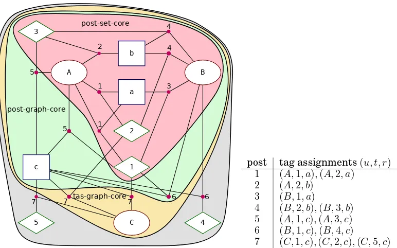
Running Example.Figure 2 shows an exemplary folksonomy hypergraph with users
A, B, C (drawn as ), resources a, b, c ( ), and tags 1,2,3,4,5 ( ) which are
[image:9.612.188.427.91.146.2]de-B
C A
a b
c 1
2 3
4 5
post-set-core
tas-graph-core 1 1 2
3 4
4
5
7 5
6 6
7 7
post-graph-core
post tag assignments(u, t, r) 1 (A,1, a),(A,2, a)
2 (A,2, b) 3 (B,1, a)
4 (B,2, b),(B,3, b) 5 (A,1, c),(A,3, c) 6 (B,1, c),(B,4, c)
7 (C,1, c),(C,2, c),(C,5, c)
Fig. 2. A folksonomy toy example with a tas-graph-core, post-graph-core, and post-set-core. The table on
the right lists the tag assignments that belong to each post.
picts the number of the post the tag assignment belongs to. The differently colored ar-eas that enclose parts of the graph depict the various types of cores that are explained in the sequel.
2.3.1. The Tas-Graph-Core of a Folksonomy.We can regard the folksonomy F =
(U, T, R, Y)as a hypergraphG= (V, E) := (U ·∪T ·∪R, Y). Together with the levell∈N
and the vertex property function
p:V ×P(V)→N: (v, W)7→
|({v} ×T×R)∩E|W| if v∈U |(U× {v} ×R)∩E|W| if v∈T |(U×T× {v})∩E|W| if v∈R
(3)
that assigns to every W ⊆ V and every v ∈ W the number of tag assignments that
v is part of in W, we get the tas-graph-core at level l of the folksonomy F. It has the property that every user, tag, and resource is part of at leastl tag assignments. Note, that for a tag to be part of a tas-graph-core at levell, it must have been used in at least lposts, while for a user (resource) it is sufficient to annotate (be part of) only a single post with at leastltags (cf. [J ¨aschke et al. 2008]).
Running Example.Figure 2 shows thetas-graph-coreat level 2, in which every
en-tity belongs to at least two tag assignments. The tag assignments(B,4, c)from post6 and(C,5, c)from post7are lost because the tags4 and5belong each only to the one
corresponding tag assignment. Note, that the tas-graph-core does not have level 3,
since the tag assignment(C,5, c)does not belong to the tas-graph-core and thus user
Coccurs in only two tag assignments.
2.3.2. The Post-Graph-Core of a Folksonomy.To circumvent the aforementioned problem,
[image:10.612.114.500.91.332.2]Therefore, we define forv∈W ⊆V (using the same notation2as in Equation 3) a new vertex property function that counts for every entity of the folksonomy the number of
posts(instead of tag assignments, as before) it is part of:
P:V ×P(V)→N: (v, W)7→
|{(v, Tvr|W, r)|r∈R|W, Tvr|W 6=∅}| if v∈U
|{(u, v, r)∈E|W}| if v∈T
|{(u, Tuv|W, v)|u∈U|W, Tuv|W 6=∅}| if v∈R
This definition intuitively violates the symmetry of the ternary structure of a
folkso-nomy. This can be seen from the property functionP, where – in contrast to the
previ-ous core – the value for tags (v ∈T) is no longer defined analogously to the values for users and resources. This is because one post always contains exactly one user and ex-actly one resource but can have more than one tag. However, the post-graph-core more closely resembles the view of a folksonomy as ‘a collection of posts’ that collaborative
tagging systems typically provide. The post-graph-core at levellhas the property that
each user, tag, and resource occurs in at leastl posts. We illustrate in Section 3 that post-graph-cores have been frequently used in the evaluation of recommender systems for folksonomies.
Running Example.In the example in Figure 2 we can see that in the
post-graph-coreat level 2 every entity belongs to at least 2 posts. Due to the removal of the userC (which only belongs to post7), all tag assignments from post7(and thus the post itself) are removed. Similarly, tag4is removed as it belongs only to post6.
Diminished Posts in Tas-Graph-Cores and Post-Graph-Cores.In the previous two
constructions, the core is computed by removing single tag assignments. Thus, from one post, several tag assignments can be removed, while others (of the same post) re-main in the core. This rather unfortunate behavior is illustrated in Table II using a
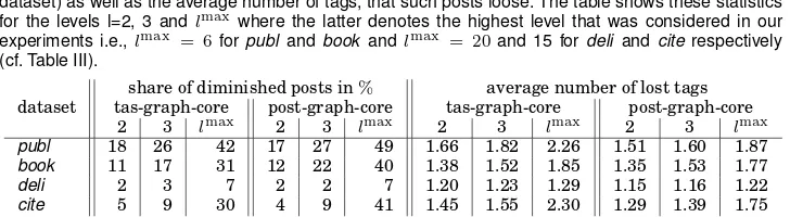
post from the BibSonomybook dataset which we use and describe in Section 4.1. The
post (that is also shown in Figure 1) consists of five tag assignments in the original da-taset. By restricting the data to a tas-graph-core or a post-graph-core, some of these tag
assignments are omitted and the post is diminished. In the tas-graph-core at level 2,
first the two rare tags “requetes” and “webmetrics” vanish from the post. At level3and also in the post-graph-cores, also the tag assignment with the tag “comparateur” is re-moved. The tags “statistics” and “trends” are well connected with other folksonomy entities through tag assignments in other posts. Thus they remain in the cores for sev-eral levels until the complete post vanishes from the dataset at levels higher than 12 for tas-graph-cores and levels higher than 5 for post-graph-cores.
Running Example.In our running example we can also observe a diminished post.
In the constructions of both the tas-graph-core and the post-graph-core post6is dimin-ished: tag assignment(B,1, c)still belongs to the core, while tag assignment(B,4, c)is
removed. Thus post6has now only one tag, instead of the original two.
The use of set-cores now allows us to overcome the phenomenon of diminished posts by regarding posts as atomic entities. We call this new construction thepost-set-coreof a folksonomy:
2.3.3. The Post-Set-Core of a Folksonomy. LetS be the set of all posts inFand for some
subsetS˜⊆Sof posts letS˜u,S˜t,S˜rbe the sets of posts inS˜, that a useru, a tagt, or a resourceroccurs in, respectively. Note, that these can be empty sets, if the according
2U|
W,R|W,T|W,Tvr|W, andTuv|W denote the restrictions ofU,R,T,Tvr, andTuv, respectively, to the
Table II. An example post from thebookdataset (cf. Section 4.1) that is diminished by the construc-tion of cores. In the post – stored by a user with ID 1015 – the resource is a bookmark to the URL http://www.google.com/trends and the post was annotated with five tags (see also Fig. 1). Through the core constructions, some tags are removed from the data, while others remain (column “tags”)
leaving the post diminished in the respective core. Finally for tas-graph-cores at levelsl≥13and
post-graph-cores at levelsl≥6the post vanishes completely from the core.
core tags
full dataset statistics, trends, comparateur, requetes, webmetrics tas-graph-core at levell= 2 statistics, trends, comparateur
tas-graph-core at level3≤l≤12 statistics, trends post-graph-core at level2≤l≤5 statistics, trends
entity ofFdoes not occur in any post contained inS˜. Now, the functions
p˜S: ˜S→N3: (u, Tur, r)7→
|S˜u|, min t∈Tur
|S˜t|,|S˜r|
are monotone in the way required by Theorem 2.3 (where N3 is partially ordered as
usual by (a1, b1, c1) ≤ (a2, b2, c2) ⇐⇒ a1 ≤ a2, b1 ≤ b2, c1 ≤ c2). The monotonicity simply follows from the observation that by shrinking S˜ the setsS˜u,S˜t and S˜r can loose but never gain cardinality.
The functions assign to each post a triple: the number of posts each of the post’s entities is part of within the subsetS˜. For any vector l ∈ N3 we can now construct a
post-set-coreas a set-P-core atl. In particular, this notion of core allows us to select
three different thresholds(lu, lt, lr)∈N3 for the number of occurrences of users, tags, and resources, respectively. The following examples illustrate use cases for choosing different thresholds:
— When one goal of a tag recommender is to consolidate the tag vocabulary of the
system, a large threshold lt ensures that only frequently used tags remain in the
dataset for evaluation. The thresholdsluandlrcan remain low.
— If the cold-start problem for users and resources shall be neglected in the evalua-tion, high values forluand/orlrcan be selected whileltcan be low.
For the sake of simplicity, we say that a post-set-core is of levellwhen all three thresh-olds are equal tol.
Running Example. Thepost-set-coreat level(2,2,2)is shown in Figure 2, where
ev-ery user, tag, and resource of the four posts1,2,3, and4belongs to at least two of these four posts. The example also illustrates an important property of the post-set-core con-struction: None of the remaining posts is diminished, all remaining posts are complete in the sense that they still contain all the tags they have in the original dataset, as each post as a whole is treated as an atomic part of the dataset. This is neither the case for the tas-graph-core (e.g., post 7 loses tag 5) nor in the post-graph-core (post 6 loses tag 4), since here the posts are modeled as collections of tag assignments and tag assignments are removed individually during the core construction.
The example in Figure 2 illustrates the property that a tas-graph-core always con-tains the post-graph-core at the same level, and the latter concon-tains all posts of the post-set-core at that level. This property follows directly from the core construction and is formalized in the following lemma.
LEMMA 2.5. Given a folksonomyFand a levell∈N.
(1) Each user u, tag t, and resource r, as well as each tag assignment (u, t, r) of the
(2) For each post(u, Tur, r)in the post-set-core at levell, the entitiesu,r, andt∈Tur, as
well as all tag assignments(u, t, r)(fort∈Tur) are contained in the post-graph-core
at levell.
Finally, a trivial example for each core type is the 1-core, which is the full folkso-nomy itself, excluding isolated nodes (e.g., users that registered with the system but never used it and thus do not occur in a post). Tag recommender evaluation usually ig-nores isolated nodes and therefore the cores at level 1 are just the original evaluation datasets (in the following also referred to as theraw data).
Similar Constructions on Other Data.The core constructions described for
folkso-nomies can easily be generalized to other similar data structures where entities have
some countable properties. For example a tweet in the micro blogging system Twitter3
consists of a user, URLs, hashtags, and several words. Much like in the case of
folkso-nomies we can derive countable properties for each tweett, e.g., the minimum number
of tweets the URLs of t occur in, the minimum number of tweets that each hashtag
of toccurs in, or the minimum number of tweets each word of t occurs in, etc. Using
a set-core like in 2.3.3, we can then simply impose individual thresholds on the URL, hashtag or word frequencies. Depending on the particular use case, one might, for ex-ample, set high thresholds on the hashtag and URL frequencies to select only trending topics and resources, while setting a low threshold for words. Moreover, it would be possible to combine two aspects, say URLs and hashtags, by using maps that count
the number of tweets that share either the URL or a hashtag with a tweett.
In contrast to the use of set-cores, graph cores would require to impose a graph structure first, e.g. by connecting all entities of a tweet by 4-dimensional hyperedges where each edge connects the user to one of the hashtags, to one of the words, and to one of the URLs of a tweet. Other than with set-cores however, such graph-cores would yield “diminished tweets” (e.g., missing some infrequent words or hashtags). Furthermore, since including URLs or hashtags in a tweet is optional, the graph model would have to be able to deal with tweets that do not contain all these components, e.g., by using edges of different dimensionality.
3. RELATED WORK
In this section, we review and discuss several examples from the literature that deal with the topics of this work. We start with the previous use of cores in various areas of research before we turn our attention to the evaluation of recommender systems. We
discuss the well-known problem ofsparse data, which can be tackled by focusing on
the dense part of the data, e.g., by usinggraph cores. Since the latter is often the case in the benchmarking of tag recommender algorithms we review the state of the art in that area next, covering different approaches as well as variations in the experimental setups. Finally, we compare several previous tag recommender benchmarking studies regarding their use of cores.
Graph Cores.One widely applicable methodology to create dense subsets of graphs
are the so-called graph-cores which were introduced by Seidman [Seidman 1983].
Batagelj and Zaverˇsnik [Batagelj and M. Zaverˇsnik 2002; Batagelj and Zaverˇsnik
2011] extended this work by introducing generalized cores– see Section 2 for details.
Cores have previously been used to create generative models of graphs [Baur et al. 2007] or to improve the visualization of large networks [Ahmed et al. 2007]. Angelova et al. [Angelova et al. 2008] analyzed cores of various derived graphs (friendship, com-mon entities, and similarity graphs) of a social bookmarking dataset. The number of
connected components quickly drops to one, already for small core levels. In general, an increasing core level results in a decreasing average node distance and a more com-plex behavior of the average clustering coefficient. In [Wang and Chiu 2008], cores of a transaction network of an online auction system were used to identify densely connected subgraphs of malicious traders in order to recommend trustworthy auction sellers. By now, cores are an established methodology to analyze the structure and dy-namics of graphs with applications as diverse as, e.g., community detection [Giatsidis et al. 2011], temporal analysis of the internet topology [Alvarez-Hamelin et al. 2005], or the study of large-scale software systems [Zhang et al. 2010]. Our generalization to arbitrary sets in Section 2 therefore opens up new possibilities for core-based analyses on data other than graphs.
Evaluation of Recommender Systems. Research on recommender systems evaluation
typically focuses on the selection of proper metrics and performance criteria (like user preference, coverage, trust, novelty, etc.) as well as on data processing and selection methods. A good overview is presented in [Shani and Gunawardana 2011]. A fixed
se-lection of metrics and criteria constitutes anevaluation framework like the one
distribution that have a positive influence for some of the tested algorithms, but a neg-ative influence on the performance of others. In our experiments in Section 5.1 we can similarly observe that the properties core type and core level have an influence on the benchmarking of tag recommender algorithms and that different tag recommender al-gorithms react differently to different cores.
Sparse Data.In many recommendation scenarios, the sparsity of the data is a
clas-sical problem since it can lead to overfitting and impede the performance of recom-menders. In particular, sparse user rating data limits the identification of similar users and items in collaborative filtering [Sarwar et al. 2000]. The sparsity problem has been tackled either by dealing with the sparsity in particular or by focusing on the dense part of the data, e.g., [Sarwar et al. 2001]. A typical approach to reduce spar-sity is dimensionality reduction, e.g., via matrix factorization. For instance, [Ma et al. 2008] proposed a matrix factorization approach that combines traditional rating data with social network data to reduce the sparsity of the ratings matrix. [Sarwar et al. 2000] used singular value decomposition to compute user neighborhoods on dense, low-dimensional product matrices. Content-based approaches have also be used to increase the density of the rating matrix for collaborative filtering, e.g., [Melville et al. 2002], or have been combined with collaborative methods, e.g., [Popescul et al. 2001] using a unified probabilistic framework. Most of the approaches that focus on the dense part of the data are rather ad-hoc, e.g., by defining some threshold for the minimal num-ber of ratings an item or user should have. There are few theoretical considerations or experiments that investigate the implications of such thresholds on the performance of different recommender algorithms or the validity of the experiments. For example, [Herlocker et al. 2004] addressed the density of datasets as one of the properties that influence recommender systems evaluation. While they empirically compared differ-ent (classes of) evaluation metrics, they do not further investigate density as a factor of the evaluation. In this work, we show how using cores (to increase the density of the data) can influence the results of a tag recommender benchmarking.
Tag Recommender Systems and Their Evaluation.Since the emergence of social
bookmarking, the topic of tag recommendations has raised considerable interest of researchers such that a vast amount of related work exists. Recommending tags can serve various purposes, such as: increasing the chance of getting a resource annotated, reminding a user what a resource is about, and consolidating the vocabulary across the users. Furthermore, as [Sood et al. 2007] pointed out, tag recommenders lower the ef-fort of annotation by changing the process from agenerationto arecognitiontask, i.e., rather than “inventing” tags the user only needs to find and select a recommended tag. Here, we introduce a selection of important results and observe different experimental setups for the comparison of different algorithms.
reward-penalty algorithm. The approach was evaluated qualitatively on 18 resources (URLs). Other early works include [Basile et al. 2007], who suggested an architecture of an intelligent tag recommender system based on words extracted from the resources and a Naive Bayes classifier (no evaluation is performed), and [Vojnovic et al. 2007], who tried to imitate the learning of the true popularity ranking of tags for a given re-source during the assignment of tags by users. The method in [Vojnovic et al. 2007]
was evaluated with precision over 1 200resources, though no details about the
hold-out set are given. The mentioned approaches address important aspects of the tag rec-ommendation problem, but they diverge on the notion of tag relevance and evaluation protocol used. In [Xu et al. 2006; Basile et al. 2007], e.g., no quantitative evaluation is presented, while in [Mishne 2006], the notion of tag relevance is not entirely defined by the users but partially by experts. An extensive evaluation of collaborative filtering, the graph-based FolkRank algorithm [Hotho et al. 2006], and simpler methods based on the usage frequency of tags was performed in [J ¨aschke et al. 2008] on three datasets from CiteULike, Delicious, and BibSonomy. FolkRank outperformed the other meth-ods and a hybrid that combined frequently used tags of the user with tags that were frequently used to annotate the resource was second. The evaluation was performed
using post-graph-cores in a setup calledLeavePostOut– a variant of the leave-one-out
hold-out estimation [Herlocker et al. 2004] – where for each user a post is randomly selected and removed from the dataset while all remaining data is used for training.
The ECML PKDD Discovery Challenges 2008 and 2009 [Hotho et al. 2008; Eister-lehner et al. 2009] addressed the tag recommendation task and resulted in many new approaches. In particular, the 2009 Discovery Challenge established a common eval-uation protocol against which more than 20 approaches were evaluated: on datasets from BibSonomy, posts from the most recent six months were used as test data and the approaches were evaluated with the F1 measure over the top five recommended tags. One task focused on graph-based recommendations and ensured that every tag, user, and resource from the test dataset were already contained in training data by using a post-graph-core at level 2. The content-based task was evaluated on the complete six months of the test data. The 2nd of 2008 and winner of the 2009 content-based task [Lipczak et al. 2009] was a hybrid recommender that combined tag suggestions from six sources (e.g., words from the title expanded by a folksonomy driven lexicon, tags from the user’s profile) and re-scored them, e.g., by the frequency of usage of the posting user. The winners of the graph-based task [Rendle and Schmidt-Thieme 2009] produced recommendations with a statistical method based on factor models. They fac-torized the folksonomy structure to find latent interactions between users, resources and tags. Using a variant of the stochastic gradient descent algorithm, the authors op-timized an adaptation of the Bayesian Personal Ranking criterion [Rendle et al. 2009]. The learned factor models are ensembled using the rank estimates to remove vari-ance from the ranking estimates. Finally, the authors estimated how many tags to rec-ommend to further improve precision using a linear combination of three estimates. A novelty of the challenge was the evaluation of some algorithms in an online setup where the click-rate of BibSonomy users could be measured. There, again the recom-mender presented in [Lipczak et al. 2009] clearly outperformed other approaches. For further results of the challenges we refer to the proceedings [Hotho et al. 2008; Eister-lehner et al. 2009] and the summary in [J ¨aschke et al. 2012].
[Seitlinger et al. 2013] proposed an approach that simulates human category learning in a three-layer connectionist network. Similar to [Krestel et al. 2009], in the input layer Latent Dirichlet Allocation is used to characterize the resource (and user). [Ma et al. 2013] proposed ‘TagRank’, a variant of topic-sensitive PageRank upon a tag-tag correlation graph which they integrate into a hybrid with collaborative filtering and popularity-based algorithms. The selection of the algorithms for the hybrid is guided by a greedy algorithm. While the approaches in [Ramezani 2011] and [Seitlinger et al. 2013] were evaluated with the same setup as in [J ¨aschke et al. 2008] (using Leave-PostOut on cores and selecting one post per user at random), [Ma et al. 2013] per-formed five-fold cross validation and the results were “averaged over each user, then over the final five folds” though no details on how the data was split (e.g., per user) were given. Overall, algorithms are typically evaluated on offline datasets, the posts for the test sets are selected at random, and measures like precision, recall, and F1 are used for evaluation. There is a tendency to use the LeavePostOut methodology, though other cross-validation procedures (LeavePostOut is|U|-fold cross validation where|U|
is the number of users in the dataset) and other types of splits are also used.
Cores and Recommender Systems.As part of the evaluation of recommender
sys-tems, cores have first been used in [J ¨aschke et al. 2007] to focus on the dense part of folksonomies – the tripartite hypergraphs of collaborative tagging systems. Exper-iments with different tag recommenders were conducted on subsets of folksonomies,
constructed as generalized cores – so-called post-coreslike explained in the previous
section. Cores were then commonly used in the evaluation of (tag) recommendation algorithms for collaborative tagging systems, e.g., in [Ramezani 2011] to compare dif-ferent PageRank variants on cores from Delicious, BibSonomy, and CiteULike at levels 20, 5, and 5, respectively, in [Krestel et al. 2009] to evaluate a tag recommendation al-gorithm based on Latent Dirichlet Allocation on a core at level 100 of a dataset from Delicious, in [Seitlinger et al. 2013] to evaluate a category-based tag recommender on a Delicious core at level 14, in [Ma et al. 2013] to evaluate ‘TagRank’, a variant of topic-sensitive PageRank upon a tag-tag correlation graph on a Delicious core at level 9 and cores at level 5 from Last.fm and Movielens, and in [Nanopoulos et al. 2013] to eval-uate a matrix factorization-based song recommender with the core level set such that it is equivalent to 0.001% of the total playcounts. As mentioned earlier, a post-graph-core at level 2 of a BibSonomy dataset was also used in the ECML PKDD Discovery Challenge 2009 for the graph-based task.
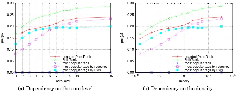
As this overview shows, the choice of the particular core level is very diverse and typically neither justified nor evaluated. The arguments for using cores are similar throughout these approaches and are summarized in [Ma et al. 2013]: “the size of each dataset is dramatically reduced allowing the application of recommendation tech-niques that would otherwise be computationally impractical, and by removing rarely occurring users, resources and tags, noise in the data can be considerably reduced.” Except for [J ¨aschke et al. 2008], all these works did neither question or challenge the use of cores nor did they compare their findings on several cores or to results on the raw data. In [J ¨aschke et al. 2008] the results on a Delicious core at level 10 were com-pared to results on a dataset where only users and resources with less than two posts were removed. Recall and precision of all algorithms except the adapted PageRank were found to be similar. Furthermore, besides the typical lack of evaluation on the raw data, all aforementioned evaluation setups suffer from the problem of diminished posts which we described in Section 2.3.2 together with a solution by introducing post-set-cores.
Summary.As we pointed out in the previous paragraphs, one commonly used
where coverage and accuracy (which correspond to recall and precision, resp.) are mea-sured. In this paper we do not aim at the evaluation of different properties of recom-mender systems nor at the presentation of a new evaluation framework. Instead, we investigate the robustness of that common evaluation framework itself and thereby challenge commonly used methodologies. Therefore (and to be comparable with previ-ous works), we investigate the influence of different core types and levels within the
fixed framework forofflineevaluation oftag recommender systemsinfolksonomies
us-inggraph coresin combination with theLeavePostOutmethod and the standard
mea-suresprecision, recall, and MAP.
A first rigorous evaluation of the influence of different types and levels of cores was performed in [Doerfel and J ¨aschke 2013]. In this paper we extend this work by per-forming a thorough assessment of the evaluation framework based on the use of cores, which has been employed in the aforementioned works. In particular, we extend [Doer-fel and J ¨aschke 2013] by 1) introducing our generalization of cores to solve the problem of diminished posts in Section 2, 2) extending the experiments to the CiteULike data-set, to new core levels, and to two new benchmarking setups (comparing recommenders on post-set-cores and on diminished posts), and 3) investigating further properties of the datasets, algorithms, and cores (Sections 4.1 (properties), 5.2, 5.4, and 5.5).
4. EXPERIMENTAL EVALUATION
The main goal of the experiments in this work is to demonstrate how benchmarking results act over different core types and levels. In the experiments we show that the quality of recommendations depends on (mostly increases with) the core level, that di-minished posts indeed occur frequently in tas-graph-cores and post-graph-cores and these posts influence the overall results, and that different core setups (different core types or levels) can lead to conflicting results in a benchmarking’s ranking of algo-rithms. Furthermore, we point to a peculiarity of using cores that arises from their use in the LeavePostOut evaluation scenario. To that end, we choose a fix evaluation setup for tag recommender algorithms – like it has been used frequently in previous studies – and apply it to four real world datasets. In that setup we then vary the cores and discuss the differences in the results using different metrics.
In this section we describe the setup of our experiments to test different evaluation procedures with different cores, levels, and metrics for tag recommender algorithms. More specifically, we
— describe four datasets from three collaborative tagging systems, namely BibSon-omy, CiteULike, and Delicious,
— explain the cleansing procedure that includes, amongst others, the removal of im-ported posts,
— show some basic properties of the datasets like size and density for different core types and levels, and
— detail which cores, evaluation protocol (LeavePostOut), metrics, and recommender
algorithms we use.
4.1. Datasets
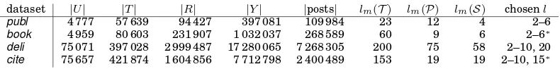
We use four datasets from three tagging systems (for an overview, cf. Table III): The
BibSonomy4dataset from 2012-07-01 is a regular dump of the system’s publicly
avail-able data.5The generation of the dataset is described in [J ¨aschke et al. 2012]. BibSon-omy supports bookmarking of both bookmarks and publication metadata, hence we
4http://www.bibsonomy.org/
Table III. The sizes of the four datasets, the levelslmof their main cores for the three different core types:
tas-graph-core (T), post-graph-core (P), and post-set-core (S), and the levels chosen for the experiments. (∗Some
levels of the post-set-core were ignored in the evaluation, cf. Section 4.2.)
dataset |U| |T| |R| |Y| |posts| lm(T) lm(P) lm(S) chosenl
publ 4 777 57 639 94 427 397 081 109 984 23 12 4 2–6
book 4 959 80 603 231 907 1 032 037 268 589 60 9 6 2–6∗
deli 75 071 397 028 2 999 487 17 280 065 7 268 305 200 75 58 2–10, 20
cite 75 657 421 874 1 604 856 7 712 798 2 400 489 153 19 19 2–10, 15∗
split the data into two parts:book andpubl. FromCiteULike6we use the official snap-shot (cite) from 2012-05-14.7FromDelicious8we use a dataset (deli) that was obtained from July 27 to 30, 2005 [Hotho et al. 2006] which is a subset of the Tagora dataset.9
Cleansing. As [Lipczak et al. 2009] pointed out, tags from automatically imported
posts are problematic for training and evaluating tag recommenders, since their prove-nance is unknown. They might have been automatically extracted from the title of a resource or resemble the folder structure of a browser’s bookmark directory and thus do not necessarily reflect the user’s view on the resource. The (in)ability of a recom-mender to predict such tags does not allow us to draw any conclusion about its per-formance on predicting user-generated tags. Moreover, in most systems, recommen-dations are usually not provided during import. Hence, we applied a similar cleans-ing strategy as described in [Lipczak et al. 2009]: we removed sets of posts that were
posted at exactly the same time by the same user. Furthermore for the cite dataset,
additional cleansing was necessary. A thorough inspection of the data had revealed that the tagsno-tag,todo mendeleyand (many different) tags likebibtex-import,
*file-import-10-07-11, or imported-jabref-librarywere frequently (and exclusively) used to
indicate imported posts. However, the posts of such an import had not identical but slightly different (consecutive) timestamps and were thus not removed by the previ-ously applied strategy. Therefore, we additionally removed all posts fromcitethat were
exclusively tagged with the tagsno-tagortodo mendeley, or a tag matching the
regu-lar expression\bimport\bor\bimported\b(where\bindicates a word boundary). In addition, we cleaned all tags as described in [J ¨aschke et al. 2012], i.e., we ignored tag assignments with the tagsimported,public,system:imported,nn,system:unfiled, con-verted all tags to lower case, and removed characters which were neither numbers nor letters.
Properties.The core construction process rapidly reduces the number of tags, users,
and resources, e.g., from 2 999 487 resources (397 028 tags) in the rawdeli dataset (cf. Table III) to 588 816 resources (65 050 tags) in the tas-graph-core at level 5. The de-cline of the number of users for an increasing core level can exemplarily be seen in
Figure 3(c). The smaller datasetsbook andpubl quickly vanish with rising core level
and although the number of users for cite anddeli is very similar, the number drops
much quicker incitethan indeli. Due to the decrease of the number of nodes,
experi-ments using cores with higher levels require a much lower computational effort since the complexity of most recommender algorithms depends on the number of entities (users, tags, and resources) or tag assignments.
Since the usual argument for the use of cores is their higher density compared to raw datasets [Krestel et al. 2009; Ramezani 2011; Nanopoulos et al. 2013; Seitlinger et al. 2013], we compare this property for all three core types on the four datasets. The
6http://www.citeulike.org/
7http://www.citeulike.org/faq/data.adp 8http://www.delicious.com/
density of a graphis often defined as the fraction of realized edges among the theoreti-cally possible edges, e.g., in [Diestel 2005] referred to asedge density. In a folksonomy, the edge density is equal to|Y|/(|U| · |T| · |R|). Other sources (e.g., [Janson et al. 2000]) define the density rather as the ratio between edges and nodes. In that case the den-sity is proportional to the average node degree in the graph. In a folksonomy the aver-age node degree is three times the edge-node ratio:3· |Y|/(|U|+|T|+|R|), since every (hyper-)edge in|Y|connects three nodes. The edge density is also related to the node degree: it can be understood as the ratio between the actual sum of degrees (in a folk-sonomy that is3· |Y|) and the theoretically possible sum of degrees (in a folksonomy that is3· |U| · |T| · |R|).
Figures 3(a) and 3(b) show for each dataset and each core type the edge density and the average node degree, respectively, depending on the chosen core level. As expected, the edge density increases with the core level and for the same level and the same dataset the post-set-core is the densest core, followed by the post-graph-core and the tas-graph-core. The average node degree at first also rises with the core level, however, with the last levels before the core vanishes we can observe a decrease for most of the cores. In the case of the tas-graph-core on the book dataset, the average node degree
drops quickly at core level 44 and then rises again at the next level. This behavior
coincides with a sharp drop of the number of users in Figure 3(c) and a sharp rise in density in Figure 3(a). An inspection of the graph properties showed that from level
43to44thebook dataset lost almost half of its remaining edges (tag assignments) but
only few nodes, while from44to45it lost two thirds of the edges but also about75%of the nodes, resulting in a much smaller and denser graph.
Comparing the behavior with respect to both density and node degree between the three core types, we see that post-graph-cores and post-set-cores are more similar to each other (especially the average node degrees are close together) than to the tas-graph-cores which always have a lower density and a lower average node degree than the other two types (compared for the same dataset and level). It is also worth noting,
that the smaller datasets (publandbook) have fewer users and lower average degrees
than the larger datasets (deli andcite), yet higher densities. This was to be expected: it is a consequence of the number of possible edges (that enters the formula for the density) which rises super-linear with the number of nodes. Among the four datasets and three core types, we can see three cores that reach the maximal density of 1: the post-set-core at level 6 of book (at level 5 the density is 826/840 = 0.98¯3), the tas-graph-core at level 45 of book, and the tas-graph-core at level96 of cite. There is no general pattern that indicates which main core has the highest density, e.g., for the publ dataset the densest main core is a post-graph-core but for thedeli dataset it is a tas-graph-core.
10-10 10-8 10-6 10-4
10-2
100
100 101 102 103
density
core level publ
book
deli
cite
(a) The density.
101 102 103
100 101 102 103
average node degree
core level publ
book deli
cite
(b) The average node degree.
100 101 102 103 104 105
100 101 102 103
users
core level
publ
book
deli
cite
(c) The number of users.
10-10
10-8
10-6
10-4
10-2
100
100 101 102 103 104 105
density
users
(d) The density over the number of users.
publ tas-graph-core publ post-graph-core publ post-set-core
book tas-graph-core book post-graph-core book post-set-core
deli tas-graph-core deli post-graph-core deli post-set-core
cite tas-graph-core cite post-graph-core cite post-set-core
Fig. 3. The density 3(a), the average node degree 3(b), and the number of users 3(c) in the graphs of the
different cores for each dataset as a function of the core level, and the density as a function of the number of users 3(d).
4.2. Evaluation Methodology
The dimensions of our experiments are the four datasets, the three different core types, the chosen levels (see Table III), the recommendation algorithms, and the evaluation metrics.
Cores and LeavePostOut. For the experiments we used – besides the raw datasets
[image:21.612.115.501.97.508.2]with most of the previous tag recommender evaluation works without particular focus on special use cases like the consolidation of the tag vocabulary (cf. Section 2.3), and, finally 3) to keep the dimensionality of the experiments manageable.
For each dataset we chose several core levels on which we conducted the experiments (see ‘chosenl’ in Table III). The difference in choice is due to the different character-istics of the datasets (size, level of the main core, unchanged cores over several levels, etc.). I.e., for the two smaller datasets (book andpubl), we selected five levels (2–6). The two larger datasets (deliandcite) allow the selection of higher levels and thus we chose consecutive levels up to level 10 and then for each dataset one larger level (20 fordeli and 15 forcite), taking into account that the cores ofcitevanish much faster than those of deli. Due to the rapid rise in density with rising core level, some cores have only very few nodes (cf. Figure 3(c)). In particular, the post-set-cores at levels 9 or higher of theciteand at levels 5 and 6 of thebook dataset contain less than 40 users. Such cores do not allow a representative evaluation of recommender algorithms, since it would rely on the judgment of very few users. They have therefore been excluded from the analyses. All other considered cores have more than 100 users.
To evaluate the recommenders, we used the variant of the leave-one-out hold-out
estimation [Herlocker et al. 2004] called LeavePostOut [J ¨aschke et al. 2007]. It is a
very common choice in tag recommender evaluation (e.g., [Ramezani 2011; Seitlinger et al. 2013; Monta ˜n´es et al. 2011; Kubatz et al. 2011]). Given a dataset (or a core), one
experiment consists of the following steps: For each useru: 1) One postpis selected
at random. 2) The post p is eliminated from the dataset and the remaining data is
used for training. 3) The task for the recommender algorithm then is to produce tag recommendations (i.e., to predict the tags ofp) given both the user and the resource of p, while the tags ofpserve as gold-standard. 4) A score is assigned that measures the prediction quality of the recommendation. This procedure is repeated for every user and the resulting scores are averaged. To ensure statistical validity, we repeated each experiment five times – such that every time a post is randomly drawn for each user – and report the averages of the resulting scores.
Evaluation Metrics. The evaluation metric determines the quality of a recommender
by measuring how successful an algorithm can predict the tags of the left-out post. We
use the two common metricsrecallandprecisionat a given cut-off levelk(rec@kand
pre@k). For a left-out postp, rec@kis the share ofp’s tags among the top kpositions
of a recommender’s ranking andpre@kthe share of the topktags in the ranking that
belong to p. In the experiments we let k run from 1 through 10. Themean average
precision(MAP) computes the arithmetic mean of the precision taken at each position
of a ranking where the recall changes. [Manning et al. 2008].
Recommender Algorithms.Since the goal of our experiments is not to find the best
algorithm, but rather to analyze the experimental setup itself, we select a set of
well-studied tag recommendation algorithms, namelymost popular tags,most popular tags
by resource, most popular tags by user, adapted PageRank, and FolkRank. Adapted
PageRank and FolkRank were first presented in [Hotho et al. 2006]. Both are adapta-tions of the original PageRank algorithm [Brin and Page 1998] to the ternary hyper-graph of folksonomies. The FolkRank algorithm computes the difference between one run of the adapted PageRank without preference (i.e., the global ranking) and one run with preference for the user/resource pair for which tags should be recommended. The latter run also constitutes the result for the adapted PageRank. We do not explore particular properties of the algorithms and therefore omit further descriptions. They can be found in [J ¨aschke et al. 2008]. In particular, we use the same parameter setting
of d = 0.7 for both the adapted PageRank and FolkRank as in [J ¨aschke et al. 2008].