Macro deformation and micro structure of 3D granular assemblies subjected to rotation of principal stress axes

DOI 10.1007/s10035-016-0632-2 O R I G I NA L PA P E R

Macro deformation and micro structure of 3D granular assemblies

subjected to rotation of principal stress axes

Xia Li1 · Dunshun Yang2 · Hai-Sui Yu3,4

Received: 30 July 2015 / Published online: 28 June 2016

© The Author(s) 2016. This article is published with open access at Springerlink.com

Abstract This paper presents a numerical investigation on the behavior of three dimensional granular materials during continuous rotation of principal stress axes using the discrete element method. A dense specimen has been prepared as a representative element using the deposition method and sub-jected to stress rotation at different deviatoric stress levels. Significant plastic deformation has been observed despite that the principal stresses are kept constant. This contradicts the classical plasticity theory, but is in agreement with previ-ous laboratory observations on sand and glass beads. Typical deformation characteristics, including volume contraction, deformation non-coaxiality, have been successfully repro-duced. After a larger number of rotational cycles, the sample approaches the ultimate state with constant void ratio and fol-lows a periodic strain path. The internal structure anisotropy

This article is part of the Topical Collection on Micro origins for macro behavior of granular matter.

Dunshun Yang—former student at Nottingham Centre for Geomechanics.

B

xia.li@nottingham.ac.uk

1 _{Room B20, Coates Building, Department of Chemical and} Environmental Engineering, Faculty of Engineering, University of Nottingham, University Park, Nottingham NG7 2RD, UK

2 _{Ove Arup, 13 Fitzroy Street, London W1T 4BQ, UK} 3 _{Nottingham Centre for Geomechanics, Faculty of}

Engineering, University of Nottingham, Nottingham, UK 4 _{State Key Laboratory of Hydraulics and Natural River}

Engineering, College of Water Resource and Hydropower, Sichuan University, Chengdu 610065,

People’s Republic of China

has been quantified in terms of the contact-based fabric ten-sor. Rotation of principal stress axes densifies the packing, and leads to the increase in coordination numbers. A cyclic rotation in material anisotropy has been observed. The larger the stress ratio, the structure becomes more anisotropic. A larger fabric trajectory suggests more significant structure re-organization when rotating and explains the occurrence of more significant strain rate. The trajectory of the contact-normal based fabric is not centered in the origin, due to the anisotropy in particle orientation generated during sam-ple generation which is persistent throughout the shearing process. The sample sheared at a lower intermediate prin-cipal stress ratio(b = 0.0)has been observed to approach a smaller strain trajectory as compared to the caseb =0.5, consistent with a smaller fabric trajectory and less significant structural re-organisation. It also experiences less volume contraction with the out-of plane strain component being dilative.

Keywords Granular materials·Discrete-element-method· Rotational shear·Internal structure

1 Introduction

motivated extensive experimental and modelling work since 1970s’.

Evidence of significance of stress rotation can be traced back to Peacock and Seed [2] who showed that the resistance to liquefaction under simple shear condition was about one third of the resistance under the analogous conditions in the triaxial apparatus. Ishihara and Li [3] devised the torsional shear apparatus and demonstrated the sensitivity of material behaviour to strain-controlled cyclic torsional shear on initial K0 and lateral confinement. Arthur et al. [4] applied

con-trolled changes of principal stress axes with the Directional Shear Cell and studied sample behaviour to shearing after a pre-loading to a high stress ratio and a rotation of princi-pal stress axes. Extensive experimental observations on sand responses to principal stress rotation have been published since the 1980s’ [5–10] using the hollow cylindrical device which offers independent control of the magnitudes and directions of principal stresses. Non-coaxial deformation and volume contraction are typical deformation characteristics observed when rotating the principal stress axes [6,7,11–15]. For constitutive theories developed for proportional load-ing, the strains can be expressed in terms of the final state of stresses, while for general loading paths involving stress rotation, the incremental theory of plasticity [16] relating increments of plastic strain to stress increments and stress history has general validity [17]. The introduction of an additional deformation mechanism associated with loading orthogonal to the current stress state is often the practice [1,18,19]. This however implies a large number of model parameters which are often difficult to calibrate.

Micromechanics and multi-scale investigation have been proven powerful during the last few decades. Calvetti et al. [20] presented the evolution of material anisotropy under complex loading condition including principal axes rotations based on laboratory tests on wooden roller stacks. Numer-ically, discrete element method (DEM) [21] has been used in numerous studies on material responses to biaxial/triaxial shearing and direct/simple tests [22–26]. Responses of two dimensional granular materials to rotation of principal stress axes have been investigated [27,28]. The trend of non-coaxial deformation and contractive volume changes have been qualitatively reproduced and explained based on struc-tural evolution.

Broadly speaking, when studying the elementary material behaviour, the specimen can be modeled as a periodic or non-periodic cell. External loading is applied on the boundary consisting of a string of boundary particles [26,28–31] or a set of rigid mass-less surfaces [21,27,32]. For particle-based boundaries, the boundary particles are often chosen accord-ing to their positions as the out-most particles. External forces can be applied directly. However, due to the highly hetero-geneous nature of particle displacements, attention should be placed on the deformation calculation. The relative

posi-tions of the particles continuously evolve as the specimen is deformed. A boundary particle at the current computa-tion step may become a non-boundary particle at the next time step based on the updated location, and vice versa. The list of boundary particles needs to be regularly updated, in particular at large strain levels. This requires additional computational power, and may also cause local force re-distribution. Alternatively, the rigid surface boundaries can be used to define the geometries of the representative ele-ment. The external surrounding interacts with the granular assembly through interacting forces arising from the overlap-ping between the boundary walls and the boundary particles. It is convenient to impose a perfectly-uniform strain field and a servo-control mechanism has been developed to achieve general loading paths. In the authors’ previous work [27], the latter has been used.

This paper aims at extending the previous work into three dimensional granulate systems, a closer analogy to real soil. Section2presents details of numerical implementation. The macro-scale deformation characteristics are to be presented in Sect.3and the observations on fabric evolution in Sect.4. Section5 extends the discussion to the effect of the inter-mediate principal stress ratio. And Sect.6draws concluding remarks from this study. In this paper, the summation con-vention over tensor indices is followed.

2 Numerical implementation

Li et al. [33] proposed a numerical technique to achieve general loading path by imposing translational and rota-tional motion of rigid fricrota-tional boundaries. In this paper, we implement it in the commercial DEM package—Particle Flow Code in Three Dimensions (PFC3D) [34] to repro-duce the material deformation characteristics to rotation of principal stress axes. For better sample uniformity, it is sug-gested that the rigid massless boundary surfaces are to be generated forming a polyhedron with obtuse angles between any two neighbouring boundaries. The boundary control algorithm detailed in [33] has been used to control the displacements of boundary walls synchronously to impose the strain-controlled boundary, and to monitor the stress-controlled boundary with a servo-stress-controlled mechanism.

A material point can be identified by its spatial position, denoted by the position vectors x and X in the deformed (current) and undeformed (reference) configurations, respec-tively. With respect to rectangular Cartesian coordinate systems x = xiei andX = XIeI, where ei(i = 1,2,3)

andeI(I=1,2,3)are the unit base vectors of the respective

reference frames. In this study, they are fixed in space and coincide with each other, i.e.,ei =eI. Because of the high

controlling material strain state. The knowledge of sample strain can be obtained from the deformation gradient tensor

F=∂x/∂X or Fi J =∂xi/∂XJ. (1)

The Biot strain definition is used to describe the specimen deformation [33]. For simplicity, in this study, we impose zero rigid body rotation, and fix the position of specimen originOthroughout the simulation. With the absence of rigid body rotation, the Biot strain becomes:

ε=1−F (2)

This is consistent with the common sign convention in soil mechanics that the positive normal strain indicates compres-sion and the negative value extencompres-sion. The Cauchy stress definition is used to describe material stress state and defined based on the boundary traction acting on current boundary configuration.

Considering the heterogeneity nature of granular materi-als, the continuum concepts, stress/strain tensors, are to be defined and calculated from the forces/displacements of the boundaries.

2.1 Strain

2.1.1 Strain evaluation

With the uniformity assumption and using Gauss’ theorem, the deformation gradient tensorFi J can be evaluated as its volumetric average, i.e.,

Fi J = 1 V

V

xi_,Jd V = −

1

V

S

xiNJd S (3)

in whichV andS are the volume and boundary surface in the undeformed configuration.NI is the unit vector normal to the boundary surface increment d S in the undeformed configuration, pointing inward and the minus sign is needed here when applying the divergence theorem. For polyhedral specimens, the specimen boundary can be discretized into a number of polygonal surfaces and the deformation gradient tensorFi J becomes

Fi J = −1 V

x_icNJS (4)

wherex_icis the area centre of surface elementSin the cur-rent deformed configuration. Once the deformation gradient tensor is obtained, the Biot strain tensor can be calculated based on Eq. (2).

2.1.2 Applying a strain increment

Sample deformation can be imposed by specifying syn-chronically the movements of boundary surfaces. This is intrinsically the strain-controlled loading mode. Denote the center and normal direction of boundary surface elementw as Xwo,Nwo in the initial configuration and xwo,nwo in the

deformed configuration, respectively. With the position of specimen origin O being fixed, the coordinate of the wall centre in the current configuration can be found as:

xoiw =Fi JXwo J. (5)

Points in the same plane in the undeformed configuration remain in the same plane after deformation. Following Eq. (5), a vectorTin the undeformed configuration becomes

ti =Fi JTJ. (6)

in the deformed configuration.

To determine the boundary wall normal directionn_owafter deformation, information of two in-plane vectorsTw₁ andTw₂ is required. The surface normal direction in the undeformed configuration can be written asNow=

Tw₁×Tw₂

Tw₁×Tw₂, where∗

represents the Euclidean normal of vector *. The two in-plane vectorst₁w andtw₂ in the deformed configuration can be calculated from Eq. (6), and used to determine the wall normal direction in the deformed configurationnwo as

nwo =

tw₁ ×t₂w

tw₁ ×t₂w. (7)

Hence, to achieve a strain incrementεI J in one time step

t, the translational velocities of the boundary surface cen-tres are to be set as:

voiw =xoi/w t =Fi JXo Jw/t = −εi JXwo J/t. (8)

To set the boundary wall rotation, we calculate the wall nor-mal direction at the current strain levelnwo and the target strain

levelnwt

o based on two in-plane vectors first. The boundary

wall rotational velocities are hence to be set as:

ww =nw×nwt/t. (9)

2.1.3 Hydro-shear decomposition

Knowing the three principal values and their respective direc-tions, the Biot strain tensor can be uniquely defined as in “Appendix 1”. A strain controlled loading path can be expressed in terms of principal strain values and directions.

and quantified. It is worthy pointing out that the summation of the principal strainsJ1(ε)is not a proper measure of volumet-ric strain. Although it provides a reasonable estimation in the case of infinitesimal deformation, the error becomes signifi-cant when the deformation is finite. The Jacobian determinant

J =det(F)relates the exact specimen volume as:

v=det(F)V = J V (10)

where v and V are the volumes in the deformed and undeformed configurations. The volumetric strain is hence expressed as:

εv= d V −dv

d V =1−J (11)

In three dimensional spaces, the deformation gradientFcan be expressed as the product of a volumetric term and a devi-atoric term as:

F=(J 1/31)

F_v

·(J−1/3

F)

Fd

=F_v·Fd (12)

Note that J(Fd) =detFd = det(J−1/3F) = J−1detF = J−1J =1, i.e., the deviatoric part is totally independent of any volume change, andJ(Fv)=detFv=det(J1/31)= J, i.e., the volumetric part contains only the information of vol-ume change [27]. Therefore, the material state of deformation can be uniquely defined by the three invariants, i.e., the vol-umetric strainε_v = d V_{d V}−dv = 1−J, the deviatoric strain

εq = 2√J2D(Fd)/3 and the intermediate principal strain ratiob_ε = ε2−ε3/ ε1−ε3alongside the three principal directionsnI

ε(I =1,2,3). Note thatbε =bF = F_F21−₋F_F33 = bF d= Fd2−Fd3

F1 d−Fd3

.

Should the loading path be specified in terms ofε_v, εq,b_ε

and the three principal directions, the volumetric defor-mation gradient tensor F_v can be determined from ε_v as F_v = J1/31 = (1−ε_v)1/31, and the deviatoric deforma-tion gradient tensorFdcan be determined fromεq,bεand the

three principal directions as introduced in “Appendix 2”. The deformation gradient tensorFcan be hence calculated from Eq. (12) and used to determine the translations and rotations of boundary surfaces to impose the specific strain-controlled loading path.

2.2 Cauchy stress

2.2.1 Stress evaluation

Cauchy stress describes the boundary forces acting over cur-rent configuration. When the representative element being

subjected to the distributed forces pi(x)applied on the cur-rent assembly boundarysand the body forcesgi(x)acting within the volumev, the average stress tensor expressed as

¯

σi j = 1

v

vσi jdvcan be evaluated as:

¯

σi j = −1_v

s

xipjds+

vρxigjdv

(13)

Note a minus is necessary when applying the divergence theorem with the inward normal direction being positive. On the local scale, the boundary traction can be viewed as discrete forces exerted at different boundary points, i.e.,

sxipjds=

β∈sxiβFβj, in whichFiβ is the external force

exerted at discrete boundary pointsβ with the coordinates of x_iβ. The body and internal forces could be estimated as

vρxigjdv=

P∈vxiPG P

j, in whichG P

i is the volumetric

force of granular particle P acting at the centre of gravity

x_iP. Hence, Eq. (13) can be discretized as:

¯

σi j = −1

v

⎛

⎝

β∈s

x_iβFβ_j + P∈v

x_iPGP_j

⎞

⎠_. (14)

This expression has be used in DEM simulate to estimate the element stress.

2.2.2 Applying a stress increment

To achieve the target stress stateσ_{i j}t, the stress increment

σi j =σt

i j−σi jis to be imposed on the specimen boundary

using the following servo-control mechanism. Expressing the stress incrementσi jin terms of its invariants(σ )I, (I = 1,2,3)and the principal directions(α_σ)I, (I = 1,2,3), the strain increment can be determined by taking analogy of an isotropic elastic constitutive relationship as:

(ε)I ₌1+ν E (σ )

I₋ ν Eσkk

(αε)I =(ασ)I (15)

where E andνare the nominal Young’s modulus and Pois-son’s ratio and(α_ε)I denotes the principal directions of the strain incrementεI J. The principal values and directions are to be used to determine the strain increment in the com-ponent form as introduced in “Appendix 1”, which is then applied on the simulated sample by specifying the boundary translational and rotational velocities as introduced in Sec-tion2.1.2.

σ, the boundary force increment over the influential area

Ais to beF =σ · A, and results in the change in the boundary-particle overlappingD =F/kn, wherekn is the particle stiffness. Estimated over the sample dimension

L, this is equivalent to the strain incrementε=D/L. To prevent overshooting of the target stress state, only a portion of the above strain incrementςε is imposed in one time step, in whichςis a relaxation factor, andς <1. The nom-inal Young’s modulus used in the simulation can hence be determined as:

E=σ /ςε=knL/ςA. (16)

In this study, it is set as default thatς =0.8 andL =2Re, whereReis the radius of the circumscribed sphere of initial sample geometry used in this study.

For a given specimen with pre-set particle properties, the nominal Young’s modulus estimated from Eq. (16) is a constant throughout the loading process. Granular material usually behaves differently from the above nominal isotropic elastic constitutive relationship. The induced change in the specimen stress state is hence expected to be different from the desired stress incrementσi j, meaning that the target stressσ_{i j}t has not been realized. In the next calculation cycle, the stress incrementσi j = σ_{i j}t −σi j is then calculated based on the updated stress stateσi j, and hence the new strain increment. By repeating doing so, the specimen stress gradually approaches the target stress state. When the dif-ference between the current stress state and the target stress state is smaller than the preset tolerance, the stress boundary condition is considered to be satisfied.

2.2.3 Hydro-shear decomposition

A three dimensional Cauchy stress tensorσ = σi jei ⊗ej

can be decomposed asσi j = σkkδi j/3+si j = pδi j +si j, in which the mean normal stress p = σii/3 = J1(σ)/3 denotes the hydrostatic pressure andsi j = σi j − pδi j is a deviatoric tensor denoting the shear stress components. Whilepitself is an invariant, the deviatoric stress tensors=

si jei⊗ej has two non-trivial invariantsJ2(s)=J2D(σ)= J2(σ) − J1(σ)2/6 and J3(s) = J3D(σ) = J3(σ) −

2J1(σ)J2(σ)/3+2J1(σ)3/27. As functions of the invari-ants are still invariinvari-ants, the shear stressq =√3J2D(σ)= σ1_−σ22_{+ σ}2_−σ32_{+ σ}1_−σ32_{/2 and the}

devi-atoric stress ratioη = q/p are also non-trivial invariants, where σ1, σ2 and σ3 denote the major, intermediate and minor principal values respectively σ1≥σ2≥σ3. In the sequel, the mean normal stressp, the deviatoric stress ratio

ηand the intermediate principal stress ratio b_σ = (σ2− σ3_)/(σ1_−σ3_{)which describes the relative magnitudes of}

the three principal stresses, together with the three

princi-pal directionsn_σI can uniquely define the sample stress state. They are used in this study to describe the loading path with rotational principal stress axes for convenience.

For a given stress state with the invariants p,η,b_σ and the principal directions n_σI, the stress Lode angle can be determined from b_σ as tanθ_σ = √3b_σ/(2−b_σ). With

J1(σ) = 3p and√J2D(σ) = ηp/√3, the three principal stresses can be expressed as

⎧ ⎪ ⎨ ⎪ ⎩

σ1_{= p1+}2 3ηcosθσ

σ2_{= p1+}2 3ηcos

2π 3 −θσ

σ3_{= p1+}2 3ηcos

2π 3 +θσ

(17)

Together with the information on the principal directions, the stress tensor in component form can be determined as in “Appendix 1”.

2.3 Polyhedral specimen geometry

For non-proportional loading paths, the tangential surface traction is required. The boundary surfaces must be fric-tional. This however increases the possibility for arching to develop between neighboring surfaces. For better uniformity, the near-spherical sample dimensions are desired. There are infinite ways to define such geometries. In 2D spaces, the convenient choice is convex regular n-sided polygons. An increasing number in sides brings the sequence of regular polygons into a circle. In 3D spaces, there are however only 5 finite convex regular polyhedron. We propose the protocol detailed in “Appendix 3” to generate a tangential polyhedron characterized by the inscribed sphere of radius Re, control-ling sample sizes, and the side numbern, defining sample shape.nis an even number andn ≥4. The angle between every two neighbouring walls is obtuse when n ≥ 6. If

n is sufficiently large, the shape of polyhedron boundary approaches a sphere. Figure1gives examples of such defined polyhedrons withn=6,n=8 andn=10, respectively.

2.4 Numerical implementations

Fig. 1 Examples of polyhedral sample geometries.an=6;bn=8;cn=10

R

1.4

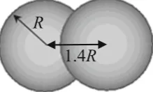
R

Fig. 2 Geometry of non-spherical particle

The linear contact model has been used with constant nor-mal and tangential stiffnesseskn = ks = 1 ×105N/m. The critical time step t used in the simulation is auto-matically determined by the minimum particle size and the contact stiffness within PFC3D. The magnitude of contact stiffness has been reduced for computational efficiency. At the maximal confining pressure, the particle overlapping is around 0.4 % of the average particle diameter and is believed small enough to satisfy the point contact assumption. The time step used in the numerical simulation is 1.02×10−6s. Sliding occurs when the tangential contact force exceeds the maximum allowable tangential forceF_maxt =μFnwith the frictional coefficient set asμ=0.5. No contact cohesion has been used. The boundaries surfaces are rigid walls with the same mechanical properties as the granular particles.

Sample preparation starts with generating spheres within the cuboidal region whose horizontal cross section is 0.0192 m×0.0192 m and height 0.133 m. 18,876 spheres have been generated. The horizontal cross section is larger than the target sample diameter to mitigate the boundary effect on packing uniformity. The cuboid is high enough to ensure no overlapping between any two of the gener-ated spheres. After generation, the spheres are replaced with clumps of equal volume and random orientations. They then deposit under the vertical gravitational acceleration

g= −100 m/s2. Local damping mechanism of PFC3D [34] has been used for energy dissipation and the magnitude is controlled by the damping coefficientξ. During deposition, the local damping has been set asξ =0.2 for dynamic sim-ulation, the particle and boundary frictions have been set as

μg=0.01 to form a dense packing. The deposition process terminates when the ratio between the unbalanced force and the average contact force ft ol = funb/fa_vis no larger than 0.01 %. After deposition, the gravity field is removed. The local damping is set asξ =0.7, and the particle and bound-ary friction coefficients are set to beμ=0.5 for the following static simulations. The specimens prepared by gravitational deposition method are anisotropic.

The boundary walls were generated inside the deposited packing to form a representative element withn =8,R =

0.0066 m. The sample size is chosen as a compromise to make meaningful observations and to achieve the large num-ber of rotation cycles required in this study. Particles with the centre of any constitutive spheres falling outside of the boundary walls are deleted. The remaining 5,188 particles form the representative element for simulation. The sam-ple is re-equilibrated by cycling with fixed boundaries until

ft ol ≤0.01 %, and then consolidated to the isotropic stress state of p = 500 kPa. The sample has been monotonically sheared in triaxial model by loading in the z axis direction. The intermediate principal stress has been fixed in the y axis direction with constant intermediate stress ratio b_σ = 0.5. The stress–strain responses are plotted in Fig.3. It exhibits dense material behavior, dilative and softening after the peak stress ratio ηp = 1.2. At large strain level, the specimen approaches the critical stress ratioηcs =0.96 and the criti-cal void ratioecs=0.70.

Fig. 3 Stress–strain responses in triaxial shearing with b=0.5

Table 1 Numerical test programme

Simulation number Stress state Void ratioe0 DEB05Y05 True triaxial

(b=0.5)

η=0.5 0.645

DEB05Y06 η=0.6 0.645

DEB05Y07 η=0.7 0.645

DEB05Y09 η=0.9 0.645

path achieved using the servo-control mechanism described in Sect.2.2.3. Loading is applied only when the sample is considered equilibrium(ft ol ≤ 0.01 %)and the boundary stress condition is closely monitored.

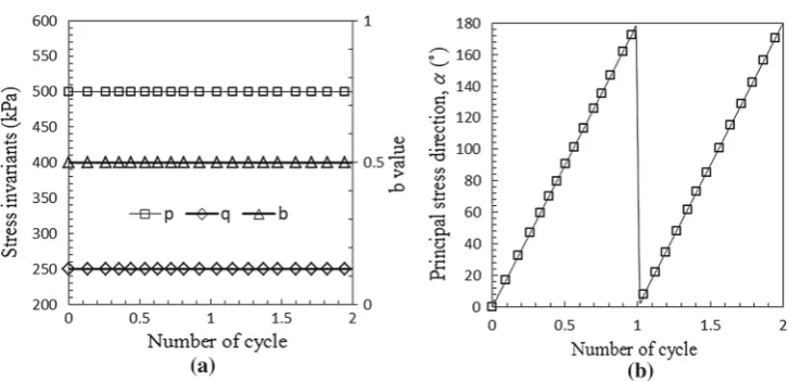
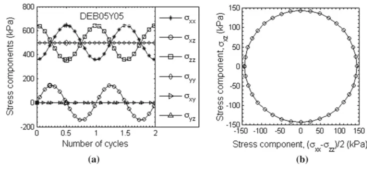
The stress paths for the simulation DEB05Y05 are plot-ted in Fig.4, confirming that the mean normal stress, the deviatoric stress and theb value have been kept constant. The deviation of the major principal stress axis to thezaxis is denoted as angleα. Figure5plots the six stress compo-nents and its trajectory in the(x,z)plane, which is a circle as expected.

3 Deformation to rotation of principal stress axes

3.1 Strain components

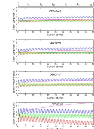
The strain developed during rotation of principal stress axes is plotted in Fig.6. The strain componentsεyx, εyzare observed to be nearly zero, indicating the y axis coincides one of the principal strain directions.εyycontinuously accumulates during rotation even though the stress component σyy has been maintained constant.εyyhas been observed to be posi-tive indicating volume contraction. A higher value ofεyyis observed at a larger stress ratio. The rate of change flattens when rotation of principal stress axes continues.

The three strain components in the(x,z)planeεx x, εx z, εzz vary cyclically. There are un-recoverable strains developed in each cycle, more significant during the first few cycles than later. These are clear evidences of plastic deformation caused by rotation of principal stress axes. Similar observa-tions have been reported in experimental hollow cylinder test results on sand [9,35].

Fig. 4 Stress invariants and principal stress directions.a

Fig. 5 Stress paths during rotation of principal stress directions.astress components,

bstress trajectory

3.2 Strain trajectories

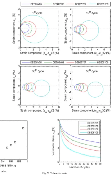
The three cyclic strain componentsεx x, εx z, εzzare plotted in Fig.7in the(x,z)plane. Only data from cycle 1, 10, 30 and 50 are extracted and plotted for clarity. Different from the circular stress trajectory, the strain trajectories are initially spiral. The vector from the start to finishing point of each cycle indicates the amount of plastic deformation, which are significant during the first few cycles. The strain trajectories gradually approaches circular and become closed as rotation continues. A larger strain trajectory is observed at a greater stress ratio, similar to previous numerical and experimental observations [8,9,27,35]. However experimental observa-tions report elliptical strain trajectories [35]. The difference may be due to the idealization in DEM simulation or the non-uniformity in developed hollow cylindrical testing, and is subject to more investigation.

The normalized strain increment defined as εR_{I J} = lim_α→0(εI J/α) has been proposed to quantify the

amount of strain increment per unit amount of stress rota-tion. With the y axis being the principal strain direction and

εR

yy plotted in Fig.6, what of interest is the deformation in

the(x,z)plane, which can be presented in terms of(ε)_vR=

εR

x x +εzz, (ε)R qR = εx xR −εzzR

2

/4+ε_{x zε}R R zx

andα_εR =atan2ε_{x z}R/ ε_zzR −ε_{x x}R/2, in which(ε)R_q equals the diameter of the osculating circle for the strain trajectories in the(x,z)plane.(ε)_qR in the 50th cycle is plotted in Fig.8showing that much more significant strain increments at higher stress ratios.

3.3 Volume contraction

The volumetric strainεvhas been plotted in Fig.9. Although the specimen is categorized as dense, and excess volume dilation occurs in monotonic shearing as shown in Fig.3, the sample contracts when subjected to rotation of princi-pal stress axes. The rate of volume contraction becomes

smaller with the number of cycles increases. Although 50 cycles are not sufficient to bring the sample into the ultimate void ratio, it is anticipated that the volume strain reaches the limit should the stress rotation continue. The specimen hence reaches the ultimate state. As previously reported, the specimen approaches a denser state at the higher stress ratio. This is similar to the experimental observation reported on the drained response of sand under rotational shear [9,35]; and shares the same mechanism with the larger pore pres-sure build-up at higher stress ratio in the undrained rotational shear [36,37].

The volumetric strain might be contributed by compres-sion in the y direction or contraction in the(x,z)plane. As observed in Fig.6,εyyis always compressive, more signifi-cant at a higher stress ratio. Comparing the volumetric strain in Fig.9andεyyin Fig.6, it is seen that the sample contracts in the(x,z)plane atη=0.5, η=0.6, η=0.7, while in the case ofη=0.9, the sample experiences significant dilation in the(x,z)planes.

3.4 Deformation non-coaxiality

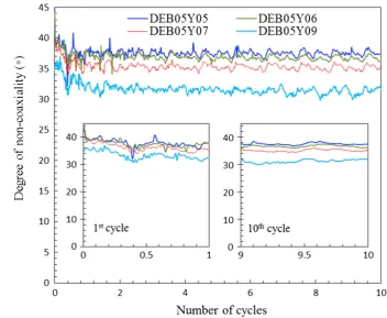
Deformation non-coaxiality is an interesting feature of gran-ular materials. The degree of non-coaxiality, defined as the difference between the normalized strain increment direction

αR

εand the principal stress directionαhas been plotted in Fig.10. The elastic strain increment is believed to be small in comparison with the plastic strain increment, the total strain increment can be used to determine approximately the plas-tic strain increment direction, as suggested by Gutierrez et al. [38]. Such an approximation is followed here for data analyzing.

coax-Fig. 6 Deformation due to rotation of principal stress direction

ial when the stress ratio gets higher, consistent with previous numerical and experimental observations [7–9,27,35].

4 Charactersation and observation of internal

structure

Discrete element simulation provides not only macro infor-mation of the representative element but also detailed data

Fig. 7 Strain trajectories at different stress ratios

Fig. 8 (ε)_qRat different stress ratios

4.1 Contact normal-based fabric tensor

It is of interest to characterize the directional distribution of contact normal density. Kanatani [39] established a

math-Fig. 9 Volumetric strain

Fig. 10 Effect of stress ratios on deformation non-coaxiality

E(n)= 1

E0 1+Di jninj

(18)

whereE0=4π,Di jis deviatoric and symmetric, referred to as the anisotropy tensor. We can further propose a function

Cp(n)= ω

E0 1+Di jninj

(19)

describing the likelihood of one particle having a contact in the directionn, whereω=Nc/Npis the ratio of contact

number over particle number, known as particle coordination number.

In this expression, two parameters are necessary to charac-terize the material internal structure.ωis an index on particle packing density andDi jcharacterizes the anisotropy in con-tact normal density distribution. They can be determined by calculating the following moment tensor:

Mi j = 1 Np

Nc

k₌1

nk_ink_j (20)

wherenk_i is thek-th contact normal vector. The coordination number can be found asω=Mii, while the anisotropy tensor

Di j can be found as

Di j =15

2

Mi j

ω −

1 3δi j

(21)

whereδi j is the Kronecker delta [40,41].

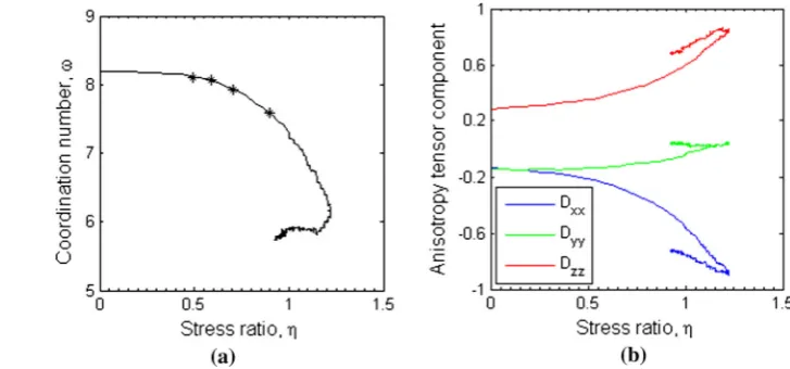
Figure11plots the evolution of particle coordination num-ber and anisotropic fabric during monotonic shearing with

b = 0.5. Upon shearing, the sample coordination number reduces while the fabric anisotropy develops. The points where stress rotation has been subsequently applied are marked with the stars.

4.2 Fabric evolution during rotation of principal stress axes

The particle coordination number during stress rotation has been plotted in Fig.12. The particle coordination number sees a trend of decreasing during the first few cycles, and then rebounding slightly while keeping cycling.

The internal structure shows a cyclic change during the rotation of major principal stress axis. The y axis remains a principal direction. During rotation of the major princi-pal stress direction, theyaxis remains as the principal fabric direction during rotation in the(x,z)plane, however there is a clear change inDyyas shown in Fig.13.Dyyis larger at the higher stress ratio, indicating a larger percentage of contact orientates in the y axis direction at the higher stress ratio.

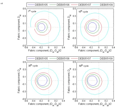
The anisotropy tensor components in the (x,z) plane have been plotted in Fig. 14 in terms of Dx z against

Fig. 11 Fabric evolution during monotonic shearing.

aCoordination number,

banisotropy tensor

Fig. 12 Evolution of coordination number at different stress ratios

Fig. 13 Evolution ofDyyat different stress ratios

the larger the fabric trajectory is, indicating the higher level of fabric re-organization. The centres of these fabric trajec-tories are seen different from the origin. As a result, the major principal fabric direction, defined as the angle between

the major principal fabric direction and the verticalz-axis,

αF, may deviate significantly the major principal stress direction.

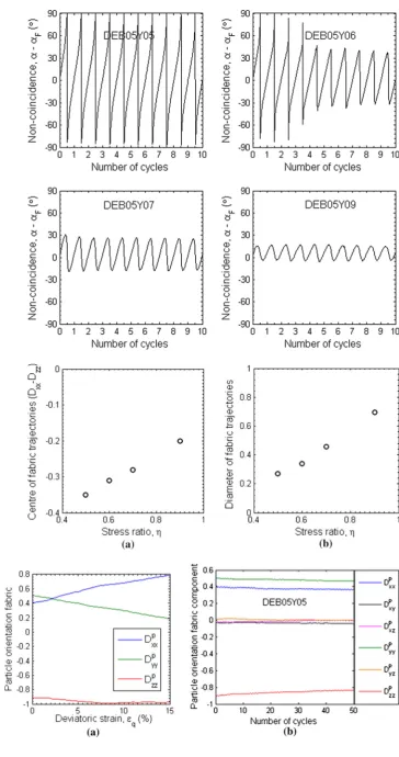
The deviation of the principal fabric direction from the principal stress direction (α−αF) has been plotted in Fig.15. At the low stress level(η=0.5), the fabric trajectory is of limited size and completely lies in the negative side of the horizontal axis. The principal fabric direction isαF =90◦ (vertical) when the principal stress direction is nearα=90◦ (vertical) as well asα=0◦(horizontal) when(α−αF)goes up nearly 90◦, as seen in Fig.16a. Higher stress ratio pro-motes more extensive structure re-organisation. The centre of fabric trajectories approaches the origin and the size of the fabric trajectories increases. The fabric anisotropy follows more closely to the stress state. The principal fabric direc-tion becomes more inclined to the principal stress direcdirec-tion.

(α−αF)varies periodically but is of a very small magnitude, as seen in Fig.16b–d.

The centres of fabric trajectory lie on the negative side of the horizontal axis, suggesting more contacts in the z axis direction than those in the x axis direction. The centre coor-dinates in the 50th cycle as well as the diameter of the fabric trajectory have been plotted in Fig.16. The centre of fabric trajectories approaches the origin as the stress ratio increases.

4.3 Anisotropy in particle orientation

Fig. 14 Fabric trajectories at different stress ratios

that the particle orientation density can be approximated by the functionEp(n)= _E1

0

1+D_{i j}pninj

. They can be deter-mined using the similar methodology of calculating contact anisotropy tensor. Anisotropy in particle orientation is plot-ted in Fig. 17. Figure 17(a) plots the information during monotonic shearing while Fig.17(b) plots particle anisotropy in stress rotation. Only data for the sample DEB05Y05 is pre-sented to exemplify the fabric evolution .

It is seen that there are very few particles orientated in the vertical z direction after deposition. In monotonic shear-ing, there are more and more particles inclined to the x axis direction as shear continues, while in stress rotation, the par-ticle orientation is persistent and only decreases slights after a larger number of cycles. With more particles lie in the horizontal plane, there are larger surface areas orientated in the vertical direction, and hence the stronger contact normal anisotropy with the z axis as the principal fabric direction.

Furthermore, an isotropic specimen has been prepared and simulated following the same loading path. The radius expansion method has been used and the prepared sample is expected to be isotropic. The void ratio prior to the rotation of principal stresses is 0.6. The sample is subjected to stress

rotation at p =500 kPa, η=0.5 andb =0.5 and labelled as REB05Y05. Its fabric trajectories are presented in Fig.18. It is evident that the specimen with isotropic particle orienta-tion has the fabric trajectory centred in the origin, confirming the offset is the results of anisotropy in particle orientation. Comparing the shape of the fabric trajectory in Fig.18and that in Fig.14, the particle orientation anisotropy seems to have little effect on the shape of the ultimate fabric trajectory.

5 Discussion on the effect of b-value

5.1 Observation of macro deformation

Fig. 15 Non-coincidence between the principal stress and fabric axes

Fig. 16 Characteristics of fabric trajectories at different stress ratios.aCentre coordinate,bdiameter

Fig. 18 Fabric trajectories of initially isotropic sample prepared by radius expansion

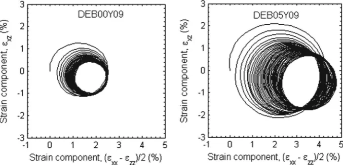
sheared atb = 0.0, η = 0.9, labelled as DEB00Y09 and DEB05Y09. The pattern is observed to be similar while sample DEB00Y09 experiences less irrecoverable plastic deformation, and also approach a circular strain trajectory. The size of strain trajectory forb =0.5 is generally larger than that withb = 0, indicating a larger strain increment rate at a greaterb value during rotational shear. And the principal direction of strain increment aligns more in the stress increment direction, as shown in Fig.20, consistent with experimental study [15,28].

The volumetric strain of the two specimens is compared in Fig. 21a while the out-of-plane strainεyy is plotted in Fig.21b. Sample DEB00Y09 is less contractive than sam-ple DEB00Y09, consistent with the experimental observation [15,28]. It is interesting to note that the sample sheared at low

bvalue(b = 0.0)experience a dilative strain in the out-of the plain withεyybeing negative while sheared at a higherb

value(b=0.5), εyyis highly contractive. In the (x,z) plane, DEB00Y09 behaves highly contractive, while DEB05Y09 behaves slightly dilative.

Fig. 20 The effect of b value: degree of non-coaxiality

5.2 Observation on fabric evolution

As shown in Sect. 4, the contact-based fabric tensor has a close correlation with stress rotation. The fabric compo-nentsDx x,Dx z,Dzzof the two specimens, DEB00Y09 and DEB05Y09, are plotted in the deviatoric space, as shown in Fig.22. The centres of the fabric trajectory locate in the negative side of the horizontal axis due to effects. As dis-cussed in Sect.4.3, this is the result of particle orientation anisotropy formed during deposition, as a result, there are contacts being more likely formed in the vertical direction. The fact that the two centres are in a similar position further confirms the hypothesis.

The fabric trajectory of DEB00Y09 approaches a circle, which is smaller than that of DEB05Y09. Viewing the change in the contact normal anisotropy as a measure of internal

Fig. 21 The effect of b value on volumetric strain.a

Volumetric strain,bεyy

Fig. 22 Effect of b value: fabric trajectory

structural re-organisation, a smaller fabric trajectory suggests less significant deformation, as observed in Fig.19.

The evolution of the coordination number and the out-of the plane fabric component during rotational shear are shown in Fig.23. After monotonically sheared up to stress ratio η = 0.9, the coordination number of DEB00Y09 is higher than that of DEB00Y09, and remains larger during stress rotation. The evolution of the out-of plane fabric com-ponentDyyis however opposite. The stress rotation causes a gradually increase inDyyfor the sample with a higher b value b=0.5 but a continuous reduction in sample DEB00Y09.

6 Concluding remarks

The virtual experiment procedure proposed by Li et al. [33] has been implemented in the commercial software PFC3D to reproduce the behavior of three dimensional granular mate-rials subjected to continuous rotation of principal stress axes. The samples are considered as the representative elements. The sample deformation is described using the Biot strain and quantified via boundary surface movements. The stress state is described in terms of the Cauchy stress tensor and

quantified with the boundary-wall interactions. The samples are initially tangential polyhedron.

Numerical simulations have been carried out. A dense specimen has been prepared using the deposition method and sheared up to different stress ratios and then subjected to continuous rotation of principal stress axes. Significant plastic deformation has been observed despite that the prin-cipal stresses are kept constant. This contradicts the classical plasticity theory, but is in agreement with previous labora-tory observations on sand and glass beads. It confirms the capability of the developed numerical technique as a useful tool to facilitate multi-scale investigation on the constitu-tive theories of granular material. The specimen shows a more contractive behavior at the higher stress ratio, which is partially contributed by the compressive out-of-plane strain component εyy. The strain rate direction fells between the principal directions of stress and stress rate. After a larger number of rotational cycles, the sample approaches the ulti-mate state with constant void ratio and periodic strain path.

Fig. 23 The effect of b value: coordination number.a

Coordination number,b

anisotropy fabric component Dyy

a large number of cycles, they approach the periodic tra-jectories in the (x,z)plane, associated with the observed strain trajectories. The larger the stress ratio, the structure becomes more anisotropic. The fabric trajectory become larger, suggesting more significant structure re-organization and explaining the larger strain rate.

Since the samples have been preparing by depositing non-spherical particles, a significant anisotropy in particle orientation has been observed. The likelihood to form con-tact in the vertical direction is increased. The concon-tact normal anisotropy is hence inclined in the z axis direction. This causes the shift of the fabric trajectory towards the minus

(Dx x −Dzz) side. Upon continuous rotation, the particle anisotropy weakens, but very slowly.

Simulation has also been conducted to study the effect of the intermediate principal stress ratio. The sample sheared at a lower intermediate principal stress ratio(b=0.0)has been observed to approach a smaller strain trajectory as compared to the caseb=0.5, consistent with a smaller fabric trajectory and less significant structural re-organisation. It also expe-riences less volume contraction with the out-of plane strain component being dilative. Observations on micro-structure and macro-behaviour provide valuable insights for develop-ing the micro-mechanics based constitutive models in order to realistically capture the behavior of granular materials under general loading paths.

Appendix 1: Tensor invariants

A three-dimensional symmetric second order tensorA =

Ai jei ⊗ ej possesses three such invariants, J1(A) = tr(A)= Aii,J2(A)= Ai jAj i/2,J3(A)= Ai jAj kAki/3,

and three mutually orthogonal principal directions.Ai j can be decomposed as Ai j = Akkδi j/3+ai j = mδi j +ai j,

in whichm = Aii/3 = J1(A)/3 denotes the hydrostatic mean,mδi j is the isotropic part, andai j = Ai j −mδi j is a trace-less term. Whilemitself is an invariant, the deviatoric stress tensor a = ai jei ⊗ej has two non-trivial

invari-ants J2(a)= J2D(A)= J2(A)−J1(A)2/6 and J3(a)=

J3D(A)=J3(A)−2J1(A)J2(A)/3 +2J1(A)3/27. A three-dimensional symmetric second order tensorA=

Ai jei ⊗ ej can also be written in the spectral form as

A=3_I=1AInI_A⊗nI_AwithAI(I =1,2,3)being the prin-cipal values and nI_A(I =1,2,3) being the corresponding principal directions, which are mutually orthogonal. Follow-ing the convention in mechanics, the superscripts 1, 2 and 3 are assigned to the major, intermediate and minor prin-cipal values, respectively A1≥ A2≥A3. Knowing the principal valuesAIand the corresponding directionsnI_A, the tensor in component form Ai j can be determined from the

principal tensorB =

A1_{0 0} 0 A20 0 0 A3

and the rotation matrix

Ri j =

_n1 1n12n13

n2₁n2₂n2₃ n3

1n32n33

, wherenI_j represents thej-th component

of the principal directionnI_A, using the following transfor-mation:

Ai j =Ri kTBklRl j (22)

Appendix 2: Calculating the deviatoric deformation

gradient tensor F

When the invariantsεq,b_εand the principal direction being specified, we can determine the deviatoric deformation gradi-ent tensorFd. First, calculate the Lode angle(0◦≤θ≤60◦)

tanθ=tanθF d =tanθ_ε =

√

3b_ε

(2−b_ε) (23)

J2D(Fd) can be determined from εq as √J2D(Fd) =

√

J2D(ε) = √3εq/2. Denotinga = √2

3

√

J2D(Fd)cosθ,

b= √2

3

√

J2D(Fd)cos 2₃π −θandc= √2

3

√

J2D(Fd)cos 2π

3 +θ

, we have the three principal values written as:

F_d1= J1(Fd)

3 +a,F

2 d =

J1(Fd)

3 +b,F

3 d =

J1(Fd) 3 +c

(24)

wherea+b+c=0,ab+bc+ca= −J2D(Fd) ,abc= J3D(Fd). Note that when the deformation is isotropic,

√

J2D(Fd)=0, andJ1(Fd)=3.

Since the determinant ofFd is equal to 1, i.e.,J(Fd)=

1,J1(Fd)can be found by solving the cubic equation

J(Fd)=(x+a) (x+b) (x+c)

=x3−J2D(Fd)x+J3D(Fd)=1 (25)

wherex = J1(Fd)

3 is denoted for convenience. The

discrim-inant of Eq. (25) is= −J2D(Fd)3 27 +

[J3D(Fd)−1]2

4 . For the

practical range of deformation in material stress–strain study,

>0. Hence Eq. (25) has only one real root, which is:

x=

−J3D(Fd)−1

2 +

√

1/3

+

−J3D(Fd)−1

2 −

√

1/3

(26)

Oncexand equivalentlyJ1(Fd)are determined, the three

principal values can be found from Eq. (24). Together with information of principal directions, the deviatoric deforma-tion gradient tensorFd can be calculated as introduced in

“Appendix 1”.

Appendix 3: Polyhedral specimen

The specimen boundary is constructed such that:

(a) The polyhedron has a top face and a bottom face. They both are parallel to the x–y plane, and referred to as the end walls. The end walls are made to be regularn-sided polygons. The vertices of the two end walls share the same(x,y)coordinates. The projection of the polyhe-dron in the(x,y)plane is shown as Fig.24a, in which the end walls are marked in shadow. In this example, the coordinates are normalized byR andn = 10. The distance between the two end walls is set as 2R. The

two end walls are centred at (0, 0, R)and(0,0,−R), respectively.

(b) Take a line passing through the mid-points of a pair of parallel sides, as the dashed line in Fig.24a. The plane formed by this dashed line and the z axis is set as a symmetric plane of the polyhedron boundary. It inter-sects the specimen boundary and forms also a regular

n-sided polygon, whose radius can be also easily found asR, shown in Fig.24b. Denoting =180◦/n, the side length of this vertical polygons isL=2Rtan. (c) In total, we can haven/2 such vertical symmetric planes

andn/2 vertical polygons. Due to symmetry, the vertices of these vertical polygons, such as pointA, A’, B, B’, C

andC, lie onn/2 horizontal planes, as seen in Fig.24b. Also the set of vertices on the same horizontal plane lie on the same circle, as in Fig.24a. Since the two sides of the vertical polygon lies in the end walls and are the diameters of the inscribed circle of the two end wall polygons, we can find the side length of the two end wall polygons asl =2Rtan2.

(d) Using this circle as the inscribe circle, we can define a

n-sided regular polygon whose sides are parallel to those of the end walls. As such we have in totaln/2n-sided regular polygons, including the two defined in Step 1, as shown in Fig.24a. The total number of vertices of the polyhedron isn2/2. For convenience, we label the vertex sequentially as shown in Fig.25.

The superscript indicates the vertex ID number. It starts in the top layer and goes counter-clockwisely with the ID assigned from 1 tonsubsequently, and then continues in the layer one level lower. The vertex in thei-th layer can be denoted byv[(i−1)n+j]wherei ranges from 1 to

n/2 and jranges from 1 ton. Looking into the horizon-tal projections, the vertices sharing the same j have the equal angular coordinates.

(e) Using thesen2_{/2 vertices, we construct a convex}

poly-hedron, which is used in the simulations here as the specimen initial boundary. The faces of the specimen boundary, besides the two end walls, are referred to as the side walls. There are (n/2−1)n side walls, which are quadrangles of four vertices and are tangen-tial to the inscribed sphere. For convenience, they are labelled top-down and counter-clockwisely. As shown in Fig.25, the side wall formed by the four vertices

v1_{, v}n_{, v}n+1_{, v}2n_{is given the ID 1. Following this}

Fig. 24 The protocol to generate a tangential convex polyhedron.aThe horizontal projection,bthe vertical intersection

-1 -0.5 0 0.5 1

-1 -0.5 0 0.5 1 O y x C' A' B' A B C

-1 -0.5 0 0.5 1

-1 -0.5 0 0.5 1 z x L=2Rtan O R B' C' A' A C B θ θ θ

(a) (b)

-1 -0.5 0 0.5 1

-1 -0.5 0 0.5 1 y x

O _W1 _Wn

1 j

v

1 n j

v

j v n j

v

_v

2

n v +

3n v

2 1n

v

2 2n

v

v vn+1

Fig. 25 Labelling the vertex and the side walls with IDs

walls are labelled as ID [(n/2−1)n+1] and ID [(n/2−1)n+2].

In 3D spaces, a plane can be generated by specifying the coordinates of a point on the place and the normal direction. In DEM softwares, a rigid wall boundary can be normally defined by a point on the surface and a unit direction. Using the spherical coordinate system, a unit direction tensor can be represented by an inclination angleθand an azimuth angleϕ. In respect to the symmetry of the polyhedral boundary, for the side wall with ID [(i−1)n+j], it can be easily determined thatθw =2i· andϕw=2(j−1)·. The tangent point of the side wall on the sphereXwt can hence be represented

by its spherical coordinates(R,2i·,2(j−1)·). Since the polyhedron defined as above is a tangential polyhedron inscribed by a sphere of radiusRand centred in the originO, all the side walls are tangent planes to the inscribed sphere. The out normal direction of the side wall can be found as nw = Xtw/Xwt , where∗denotes the Euclidean norm,

representing the length of vector * . The side wall plane can hence be determined as x−Xw×nw =0, or equivalently

x−Xw_t ×Xw_t = 0. For the two end walls, the tangent points are their centres, (0, 0, R)and (0, 0,−R), with the normal direction being (0, 0, 1) and(0,0,−1), respectively. This hence allows the generation of the complete set of wall boundaries. Loading is applied by imposing a translation velocity to the wall centres and the rotational velocity to the wall normal directions.

Acknowledgments The work reported in this paper forms part of a general research programme on non-coaxial plasticity and micro-mechanics of geomaterials carried out at the Nottingham Centre for Geomechanics. The financial support from the UK’s Engineering and Physical Science Research Council (EPSRC) and the University of Not-tingham through the Early Career Research and Knowledge Transfer Award is gratefully acknowledged.

Open Access This article is distributed under the terms of the Creative Commons Attribution 4.0 International License (http://creativecomm ons.org/licenses/by/4.0/), which permits unrestricted use, distribution, and reproduction in any medium, provided you give appropriate credit to the original author(s) and the source, provide a link to the Creative Commons license, and indicate if changes were made.

References

1. Li, X.S., Dafalias, Y.F.: A constitutive framework for anisotropic sand including non-proportional loading. Geotechnique54(1), 41– 55 (2004)

2. Peacock, W.H., Seed, H.B.: Sand liquefaction under cyclic loading simple shear conditions. In: Proceeding of ASCE, vol. SM3, pp. 689–707 (1968)

3. Ishihara, K., Li, S.I.: Liquefaction of saturated sand in triaxial tor-sion shear test. Soils Found.12(2), 19–39 (1972)

4. Arthur, J.R.F., Chua, K.S., Dunstan, T.: Induced anisotropy in a sand. Geotechnique27(1), 13 (1977)

5. Symes, M.J., Hight, D.W., Gens, A.: Investigating anisotropy and the effects of principal stress rotation and of the intermediate principal stress using a hollow cylinder apparatus. In: IUTAM Conference on Deformation and Failure of Granular Materials, pp. 441–449 (1982)

7. Gutierrez, M., Ishihara, K., Towhata, I.: Flow theory for sand rota-tion of principal stress direcrota-tion. Soils Found.31, 121–132 (1991) 8. Nakata, Y., Hyoda, M., Murata, H., Yasufuku, N.: Flow deforma-tion of sands subjected to principal stress rotadeforma-tion. Soils Found.

38(2), 115–128 (1998)

9. Tong, Z.X., Zhang, J.-M., Yu, Y.L., Zhang, G.: Drained deforma-tion behavior of anisotropic sands during cyclic rotadeforma-tion of stress principal axes. J. Geotch. Geoenviron. Eng.136(11), 1509–1518 (2010)

10. Cai, Y., Yu, H.S., Wanatowski, D., Li, X.: Non-coaxial behaviour of sand under various stress paths. J. Geotech. Geoenviron. Eng. ASCE37(1), 75–96 (2013)

11. Arthur, J.R.F., Chua, K.S., Dunstan, T., del Rodriguez, C.J.I.: Prin-cipal stress rotation. Proc. Am. Soc. Civ. Eng.106, 421–434 (1980) 12. Ishihara, K., Towhata, I.: Sand response to cyclic rotation of prin-cipal stress directions as induced by wave load. Soils Found.23(4), 11–26 (1983)

13. Symes, M.J., Gens, A., Hight, D.W.: Drained principal stress rota-tion in saturated sand. Geotechnique38(1), 59–81 (1988) 14. Joer, H.A., Lanier, J., Fahey, M.: Deformation of granular materials

to rotation of principal axes. Geotechnique48(5), 605–619 (1998) 15. Yang, Z.X., Li, X.S., Yang, J.: Undrained anisotropy and rotational

shear in granular soil. Geotechnique57(4), 371–384 (2007) 16. Drucker, D.C.: A more fundamental approach to plastic stress–

strain relations. In: Proceedings of the First U.S. National Congress of Applied Mechanics, ASME, pp. 487–491 (1951)

17. Dafalias, Y.F.: Bounding surface plasticity. I: mathematical founda-tioni and hypoplasticity. J. Eng. Mech. ASCE112, 966–987 (1986) 18. Tsutsumi, S., Hashiguchi, K.: General non-proportional loading behavior of soils. Int. J. Plast.21(10), 1941–1969 (2005). doi:10. 1016/j.ijplas.2005.01.001

19. Yu, H.S., Yuan, X.: On a class of non-coaxial plasticity models for granular soils. Proc. R. Soc. Lond. Ser. A462, 725–748 (2006) 20. Calvetti, F., Gombe, G., Lanier, J.: Experimental micromechanical

analysis of a 2D granular material: relation between structure evo-lution and loading path. Mech. Cohesive Frict. Mater.2, 121–163 (1997)

21. Cundall, P.A., Strack, O.D.L.: A discrete numerical model for gran-ular assemblies. Geotechnique29(1), 47–65 (1979)

22. Ai, J., Langston, P.A., Yu, H.-S.: Discrete element modelling of material non-coaxiality in simple shear flows. Int. J. Numer. Anal. Methods Geomech. (2013). doi:10.1002/nag.2230

23. Zhang, L., Thornton, C.: A numerical examination of the direct shear test. Geotechnique57(4), 343–354 (2007)

24. Cui, L., O’Sullivan, C.: Exploring the macro- and microscale response characteristics of an idealised granular material in the direct shear appratus. Geotechnique56(7), 455–468 (2006)

25. Thornton, C.: Numerical simulation of deviatoric shear deforma-tion of granular media. Geotechnique50(1), 43–53 (2000) 26. Ng, T.T., Dobry, R.: Numerical simulations of monotonic and cyclic

loading of granular soil. J. Geotech. Eng.120(2), 388–403 (1992) 27. Li, X., Yu, H.-S.: Numerical investigation of granular material behavior under rotational shear. Geotechnique 60(5), 381–394 (2010)

28. Tong, Z., Fu, P., Dafalias, Y.F., Yangping, Y.: Discrete element method analysis of non-coaxial flow under rotational shear. Int. J. Numer. Anal. Methods Geomech.38, 1519–1540 (2014) 29. Cundall, P.A., Strack, O.D.L.: The development of constitutive

laws for soil using the distinct element method. Paper presented at the Third International Conference on Numerical Methods in Geomechanics, Rotterdam

30. Bardet, J.P.: Numerical simulations of the incremental responses of idealized granular materials. Int. J. Plast.10(8), 879–908 (1994) 31. Thornton, C., Zhang, L.: On the evolution of stress and microstruc-ture during general 3D deviatoric straining of granular media. Geotechnique2010(5), 333–341 (2010)

32. Itasca Consulting Group Inc.: PFC2D (Particle Flow Code in Two Dimensions). In. ICG, Minneapolis, (1999)

33. Li, X., Hai-Sui, Yu., Xiang-Song, Li: A virtual experiment tech-nique on the elementary behaviour of granular materials with DEM. Int. J. Numer. Anal. Methods Geomech. 37(1), 75–96 (2013). doi:10.1002/nag.1086

34. Itasca Consulting Group Inc.: PFC3D (Particle Flow Code in Three Dimensions). In. Minneapolis:ICG, (2004)

35. Yang, L.T.: Experimental study of soil anisotropy using Hollow Cylnider testing. University of Nottingham, Nottingham (2013) 36. Nakata, Y., Hyodo, M., Murata, H., Yasufuku, N.: Flow

deforma-tion of sands subjected to principal stress rotadeforma-tion. Soils Found.

38(2), 115–128 (1998)

37. Yang, Z.X., Li, X.: Undrained anisotropy and rotational shear in granular soil. Géotechnique57(4), 371–384 (2007)

38. Gutierrez, M., Ishihara, K., Towhata, I.: Flow theory for sand during rotation of principal stress direction. Soils Found.31(4), 121–132 (1991)

39. Kanatani, K.-I.: Distribution of directional data and fabric tensors. Int. J. Eng. Sci.22(2), 149–164 (1984)

40. Kanatani, K.-I.: Distribution of directional data and fabric tensors. Int. J. Eng. Sci.22(2), 149–164 (1984)