Using 'snapshot' measurements of CH4 fluxes from an ombrotrophic peatland to estimate annual budgets: interpolation versus modelling

to estimate annual budgets: interpolation versus modelling

S.M. Green

and A.J. Baird

1_{Geography, CLES, University of Exeter, UK} 2_{School of Geography, University of Leeds, UK}

_______________________________________________________________________________________

SUMMARY

Flux-chamber measurements of greenhouse gas exchanges between the soil and the atmosphere represent a snapshot of the conditions on a particular site and need to be combined or used in some way to provide integrated fluxes for the longer time periods that are often of interest. In contrast to carbon dioxide (CO2), most

studies that have estimated the time-integrated flux of CH4 on ombrotrophic peatlands have not used models.

Typically, linear interpolation is used to estimate CH4 fluxes during the time periods between flux-chamber

measurements. CH4 fluxes generally show a rise followed by a fall through the growing season that may be

captured reasonably well by interpolation, provided there are sufficiently frequent measurements. However, day-to-day and week-to-week variability is also often evident in CH4 flux data, and will not necessarily be

properly represented by interpolation. Using flux chamber data from a UK blanket peatland, we compared annualised CH4 fluxes estimated by interpolation with those estimated using linear models and found that the

former tended to be higher than the latter. We consider the implications of these results for the calculation of the radiative forcing effect of ombrotrophic peatlands.

KEY WORDS: blanket peatland, flux chamber, methane, time-integrated fluxes

_______________________________________________________________________________________

INTRODUCTION

There is growing interest in the annual carbon

dioxide (CO2) and methane (CH4) budgets of

peatlands (e.g. Olson et al. 2013, Meng et al. 2016). Such budgeting is required for estimating the radiative forcing effect of peatlands on climate. The radiative forcing of different greenhouse gases (GHG) can be calculated using the concept of global warming potential (GWP) as defined by the Intergovernmental Panel on Climate Change (IPCC) (Myhre et al. 2013), and is usually expressed in terms of carbon dioxide equivalents (CO2-e). CH4 is a much

more potent greenhouse gas than CO2 and

correspondingly has a higher GWP. It is currently estimated that CH4 is 28 times more potent than CO2

(excluding climate feedbacks) over a 100-year timeframe (Myhre et al. 2013). Therefore, in CO2-e

terms, CH4 assumes equal importance to CO2 when

the CH4 flux in mass terms is just 3.6 % of the net

CO2 flux (e.g. Baird et al. 2009). Consequently, any

systematic under- or over-estimation of the annual flux of CH4 may have a disproportionate effect on

calculations of the radiative forcing effects of peatlands, with implications for policy and land management.

CH4 fluxes from ombrotrophic peatlands, i.e.

raised bogs and blanket bogs, are commonly

measured using flux chambers at intervals typically no less than weekly, but often fortnightly or even monthly (e.g. Waddington & Roulet 1996, Dinsmore et al. 2009, Baird et al. 2010, Moore et al. 2011). It is common to use models based on flux chamber data

to estimate annual fluxes of CO2 from bogs

(Waddington & Roulet 1996, Bubier et al. 1998, Tuittila et al. 1999, Strack & Zuback 2013, Vanselow-Algan et al. 2015). On the other hand, linear interpolation between measurements (see below) is usually used when estimating annual CH4

fluxes (e.g. Waddington & Roulet 1996, Dise et al. 1993, Roulet et al. 2007), although there are cases where models have been used (e.g. Laine et al. 2007). CH4 fluxes generally show a rise followed by a fall

through the growing season that may be captured reasonably well by simple interpolation. However, day-to-day and week-to-week variability is also often evident in CH4 flux data (e.g. Moore & Knowles

1990, Laine et al. 2007, Baird et al. 2010, Lai et al. 2014), and will not be properly represented using interpolation, in which case a modelling approach

may be preferred (see INTEGRATION

APPROACHES below). To our knowledge, interpolated and modelled estimates of time-integrated fluxes of CH4 from bogs have not been

consistently give higher values than the other?—and magnitude). To partly address this knowledge gap, we used a large flux-chamber dataset from a UK blanket peatland.

INTEGRATION APPROACHES

The integrated flux (Fg; e.g. mg m-2) of CH4 between

Time 1 and Time 2 (t1, t2) may be estimated by

interpolation using:

(

)

(

)

2 1 2 1 t t f f

F_g,− = _g, + _g, − [1]

where fg is the instantaneous flux (e.g. mg m-2 day-1).

The Fg values for each time pair may then be summed

to give an annual total. Alternatively, fg may be

modelled using environmental and ecological variables such as water-table depth, soil temperature, air temperature, and the abundance of different plant functional types. If some of these variables are measured at a higher frequency than flux chamber tests, models in which they are used can, in turn, be

run or applied to simulate fg at those higher

frequencies. The high-frequency estimates of fg can

then be summed to give an estimate of annual Fg. In

this study, we modelled fg using ordinary multiple

linear models of the following form:

ε ± + + + +

= _{n n}

g a bX b X ... b X

f _{1 1 2 2} [2]

where a and b1, b2, ...bn are fitting parameters, X1,

X2,...Xn are the independent (environmental and

ecological) variables, and ε is the model error. Multiplicative models can also be used but we found

these performed less well than models based on Equation 2. Likewise, it is possible to use biophysical

models in which the processes involved in CH4

production, consumption and transport are described in considerable depth (e.g. Grant & Roulet 2002), but very few studies are detailed enough to provide the data needed for the parameterisation and application of such models. In this study we used air temperature, soil temperature, a temperature sum index and the abundance of plant functional type as our candidate independent variables in Equation 2 (see below).

COMPARISON OF ANNUAL CH4 BUDGET

APPROACHES

Study site and methods

The study was carried out on part of the Migneint blanket bog complex in the upper Conwy catchment in North Wales (latitude 52.97 °N, longitude 3.84 °W). Site vegetation comprised a typical blanket mire assemblage including Calluna vulgaris (L.) Hull (common heather), Eriophorum vaginatum L. (hare's tail cottongrass) and various species of Sphagnum (bog mosses; e.g. S. capillifolium (Ehrh.) Hedw., S. papillosum Lindb. and S. cuspidatum Ehrh. ex Hoffm.). The peat across the sampling area was 0.54–2.39 m deep, with a pH (H2O) of 3.62–3.80,

bulk density of 0.08–0.11 g cm-3_{, loss on ignition of}

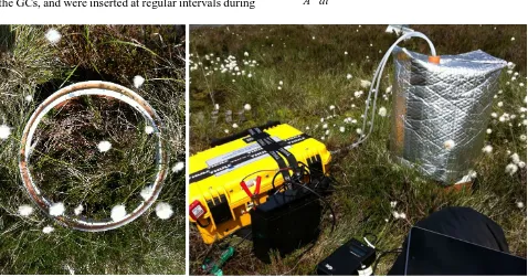
98.8–99.7 % and a C/N quotient of 30.0–36.6 (depending on depth) (Table 1). The wider purpose of the project was to investigate the effects of different methods of ditch blocking (for peatland restoration) on GHG uptake and emissions. GHG exchanges were measured across the site, both within and between ditches, using flux chambers (Denmead 2008, Green et al. 2016a). These comprised cylindrical acrylic chambers with an outside diameter

Table 1. Physical and chemical properties of the peat at the study site (n = 12). Parentheses contain standard deviation.

Depth (cm)

Dry bulk density (g cm-3₎

Volumetric water content

(cm cm-3₎

Loss on ignition

(%)

pH (H2O)

pH (CaCl2)

Conductivity

(H2O µS cm-1) C/N

0 – 10 0.08

(0.02) 0.77 (0.18) 98.8 (2.74) 3.80 (0.15) 2.98 (0.05) 61.6 (18.8) 36.6 (10.9)

15 – 25 0.10

(0.03) 0.96 (0.12) 99.6 (0.32) 3.62 (0.11) 2.97 (0.05) 81.2 (13.6) 30.0 (5.33)

30 – 40 0.11

(0.03)

0.91

(0.12) 99.7 (0.10)

(o.d.) of 300 mm, a wall thickness of 3 mm and a height of 333 mm (Figure 1) that were placed on polyvinyl chloride (PVC) collars during tests. The collars had an o.d. of 315 mm and wall thickness of 8 mm, enclosing an area of 0.07 m2_{. The collars were}

200 mm long with half that length inserted below the ground surface. The upper rim of each collar was fitted with a gutter into which water was poured and the chamber placed to form a gas-tight seal during flux tests.

Within-chamber CH4 concentrations during tests

were measured either (a) by taking syringe samples of the gas (25 mL) and later analysing these in the laboratory (see below) or (b) in-field using an on-line Los Gatos Research Ultra-portable GHG Analyzer (UGHGA; Model 915-0011; Los Gatos Research, Mountain View, California). Method (a) was used at the beginning of the project but was replaced by Method (b) in 2013 because it allowed tests to be carried out more quickly and because the UGHGA was more accurate than the laboratory method of measuring CH4 concentrations (see below). For the

syringe-sample tests (i.e. Method (a)), gas samples were taken at intervals of 1, 6, 11, 16 and 21 minutes after chamber closure. The gas samples were analysed for CH4 content using either a Perkin Elmer

Clarus 500 gas chromatograph (GC) system fitted with a flame ionisation detector (FID), or an Agilent Varian 450 GC system, also fitted with a FID. Standard analytical grade reference span gases (Cryoservice, Worcester, UK) were used to calibrate the GCs, and were inserted at regular intervals during

sample runs to check for instrument drift. When

using the Los Gatos UGHGA, CH4 concentration

readings were taken over a period of 3–5 minutes after chamber closure at a frequency of 0.5 Hz. We varied the closure time according to disturbance effects (abrupt variations in CH4 concentrations

within the chamber) associated with placing a chamber on a collar. Sometimes these effects were minimal, so we ran the test for three minutes. However, sometimes they affected readings in the first 50–100 s, in which case we ran the test for up to five minutes. Inspection of our data had shown that at least three minutes' worth of readings were required to provide a reliable flux estimate.

Changes in CH4 concentration during a chamber

test can be used to estimate the flux between the peatland and the atmosphere using (Denmead 2008):

dt d

A V

fg g

ρ

= [3]

where fg is the gas flux density at the peatland surface

(mg m-2 _day-1_{), V is the combined volume of the flux}

chamber and the collar above the peatland surface, A is the inside area of the collar (m2_), ρg _{is the mass}

concentration of the gas in the chamber (mg m-3_{), and}

t is time (days). Equation 3 may also be written in slightly modified form, as:

dt dg A

f_g = 1 m [4]

where gm is the mass of the gas in the chamber (mg)

(gm = V ×ρg).

We applied Equation 4 to our chamber data by first converting ppm gas concentrations into masses using the Ideal Gas Equation. Ordinary least squares regression (using the LINEST function in Excel 2010) was used to estimate dgm/dt by fitting a line

through the gas versus time data. The regression fit was only accepted if r2 ≥ 0.7 and p < 0.05. Fluxes for

datasets that did not meet these criteria were rejected with one exception: if variations in gas concentration during a test were within a threshold error range of the instrument being used to measure the concentrations, the flux was assumed to be zero. This range was 0.3 ppm for the GC-FID determinations (Method (a)) and 0.03 ppm for the UGHGA (Method (b)). If this additional criterion had not been used, the flux estimates would be biased to higher fluxes because all zero and close-to-zero fluxes would have failed the regression criteria and been excluded (this

additional criterion applied to ~4 % of our

measurements).

In addition to measuring gas fluxes at the study site we measured the following variables, which were candidates for inclusion in the linear models based on Equation 2 (see above).

Air temperature

This was measured at a height above the ground surface of 1.3 m using a Davis Instruments Vantage Pro 2 (Davis Instruments Corp., Hayward, California, USA) automatic weather station (AWS) situated within 100 m of the experimental area. Hourly averages of air temperature (°C) were available for use in the linear models.

Soil temperature

Soil temperature (°C) was measured by the AWS (see above) at a depth of 5 cm, and hourly averages recorded.

Temperature sum index

The temperature sum index (ETI) is the ratio of the cumulative air temperature sum to the number of temperature sum days. A threshold temperature has to be reached before the ETI is calculated. Alm et al. (1997) and Tuittila et al. (1999) estimated ETI only for that part of the year (for sites in eastern and southern Finland, respectively) when the five-day moving average air temperature was above 5 °C.

Here, we also used a temperature of 5 °C.

Mathematically, the ETI is given by:

j T ETI

j

i air,i

j 

  

  ∑ =

=1

[5]

where j is the day of interest (counted from the first day when the five-day moving average air temperature exceeds the threshold temperature), Tair

is daily-average air temperature (°C) and i is day number.

Abundance of plant functional types

The abundance of sedges (mainly Eriophorum spp.), Sphagnum spp. and ericoid shrubs was measured in each collar from digital photographs. Photographs were taken during every flux test and a subset of these were analysed for nested frequency. This measurement comprised placing a 100-cell grid over the photograph and recording the presence/absence of all sedges, Sphagnum spp. and ericoid shrubs in each cell. While this method has limitations—for example, it cannot account for layering of species— it does provide a quantitative measure of plant abundance that can be used as a predictor of CH4

exchanges between a peatland and the atmosphere.

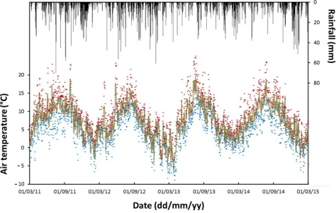
Meteorological conditions over the study period Meteorological conditions, especially rainfall, varied quite strongly over the study period (Figure 2), which ran from March 2012 to March 2015. Each project year ran from March to February; however, henceforth we abbreviate the project years according to the calendar year in which the majority of the project year fell. For each project year, the site had an annual mean air temperature of 6.5 °C (2012), 6.9 °C (2013) and 7.6 °C (2014). In the same period, the rainfall for each successive year was 2409, 1786 and 1936 mm.

Comparison of approaches to estimating time-integrated fluxes

For our comparison of integration approaches we considered CH4 fluxes from 24 of the flux chambers

deployed at the site, situated in the areas between the ditches (i.e. not within the ditch channels). Measurements were made every three to six weeks in 2012 (n=10 readings per chamber), 2013 (n=11) and 2014 (n=11) (768 flux chamber tests in total). We use the convention that positive fluxes represent emissions and negative fluxes indicate uptake. We compared estimates of annual peatland–atmosphere

CH4 emissions calculated using interpolation

Figure 2. Meteorological conditions at the experimental site between 01 March 2012 and 01 March 2015. The black bars indicate daily rainfall (mm). Average daily air temperature (°C) is denoted by the green-brown line, daily maximum temperature by the red dashes and daily minimum by the blue dashes.

there were quite large variations in model fit (see below), all of the models were included in the comparison of modelled and interpolated fluxes so that the effect of model quality (as described by SEE) on differences between the flux estimation methods could be assessed.

The models were run at hourly time intervals and the hourly fluxes summed to give annualised fluxes. The plant abundance data were obviously not available at hourly intervals, but were entered for each hour and updated for every time at which abundance was re-measured (twice per year). The training (calibration) datasets used for each model were mostly sufficiently extensive to cover the range of conditions encountered over the period of model application (i.e. 2012–2014 inclusive). The ETI and plant functional type abundance training sets included the full range of conditions encountered during the period of model application. Twelve percent of the soil temperature values during the period of application were lower or higher than the range used in the training set, while for air temperature the figure was 8.7 percent. However, in all cases where the model was applied beyond the range of the training set, the modelled CH4 fluxes

were not extreme or unreasonable.

Comparison of annualised CH4 fluxes estimated

by interpolation and modelling (Figure 3) revealed a moderate correlation (r=0.73, p<0.0001) but a significant difference between the two datasets (p=0.001) (IBM SPSS version 23: paired t-test). Interpolated fluxes were on average 29 % higher than those estimated through the modelling approach. In some cases, even the sign of the flux differs (Figure 3). The difference between the methods seems also to be related to the size of the flux, with greater differences (and scatter) at the higher end (i.e. greater than 20 g CH4 m-2 y-1). Modest-sized fluxes

(5–15 g CH4 m-2 y-1) are scattered closer to the 1:1

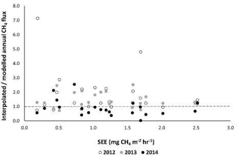
line (Figure 3). There was no correlation between the SEE of the individual flux models and the ratio of interpolated to modelled annual CH4 flux (r=-0.143,

p=0.232) (Figure 4). This suggests that model

Figure 3. Interpolated versus modelled annual methane (CH4) flux. A positive CH4 flux indicates emission

and a negative flux uptake.

Figure 4. Model standard error of the estimate (SEE) versus the quotient of interpolated to modelled annual methane (CH4) flux. Note: for 2013 there is a quotient of 77, and for 2014 a quotient of -11.2 for a model

and seasonal timing of 'snapshot' chamber measurements. In comparison, the modelling approach is dependent on the resolution and quality of the supporting datasets and the number of data points included in the model calibration dataset.

An alternative way of considering the differences in estimates between the approaches is to convert the CH4 into CO2-e and combine it with net ecosystem

CO2 exchange (NEE). To illustrate this alternative,

we considered 22 of the 24 collars for which we also had measured and modelled values of NEE (methods not explained here, see Green et al. 2016b). By combining the NEE for a collar with its CH4 flux

expressed in CO2-e we were able to estimate the

overall radiative forcing effect of the patch of peatland within the collar. The 22 collars had CH4

models with SEE in the range 0.18–2.5 mg CH4

m-2 _hr-1_{. When all 22 collars are averaged, the CH} 4

flux is estimated as 19.0 g CH4 m-2 y-1 (interpolated)

and 15.1 g CH4 m-2 y-1 (modelled), which are

comparable to CH4 annual emissions in other

ombrotrophic peatlands (Blain et al. 2014, Wilson et al. 2016). NEE for the 22 collars was estimated at -108 g CO2 m2 y-1 (i.e. a CO2 sink). When

combining the CO2 and CH4 fluxes into a single

CO2-e value, over a 100-year time frame, we

obtained a value of 424 g CO2-e m2 y-1 (CH4

interpolation) and 314 g CO2-e m2 y-1 (CH4

modelled). Notably, the difference in the CO2-e

estimates is similar to the absolute value of the NEE. Interpolation produces a 26 % increase in terms of estimated CH4 and a 35 % increase in the estimated

CO2-e flux. This is because NEE for each of the 22

collars is relatively small in magnitude, so that a substantial part of the CO2-e estimate for each collar

comprises the contribution from CH4.

CONCLUSION

Our results show that the two approaches, interpolation and modelling, can lead to substantial relative and absolute differences in estimates of peatland–atmosphere CH4 fluxes and estimates of the

radiative forcing effect of a peatland. Given the potential for such large differences, we recommend future studies on bogs take account of the effects of different integration approaches when estimating annual fluxes of CH4, and report the alternative sets

of estimates. This information is clearly policy-relevant given interest in, for example, how best to restore peatlands while also minimising CH4 fluxes

(e.g. Baird et al. 2009) and in the accurate MRV (measurement, reporting and verification) of peatland emissions and the calculation of emission factors for

land-use change in peatlands (e.g. Couwenberg 2009). In our analysis, we did not discriminate between models based on their SEE. If good (accurate) models can be developed, they are likely to provide better estimates than interpolation, unless fluxes are measured at very high frequencies (much more often than weekly, e.g. Lai et al. 2014). However, it is notable that the differential between modelled and interpolated fluxes in this study was not related to model quality or accuracy as represented by SEE. Therefore, care should be taken when deciding which approach to use.

ACKNOWLEDGEMENTS

The UK Government’s Department for Environment, Food and Rural Affairs (Defra) funded the research under grant SP1202. We are grateful to The National Trust for giving permission to work at the site. The Countryside Council for Wales (now part of Natural Resources Wales) are also thanked for funding the

vegetation survey used in the modelling of CH4

fluxes. The reviewers Markku Koskinen and an anonymous reviewer are thanked for their comments on the original manuscript which helped us improve the paper.

REFERENCES

Alm, J., Talanov, A., Saarnio, S., Silvola, J., Ikkonen, E., Aaltonen, H., Nykänen, H. & Martikainen, P.J. (1997) Reconstruction of the carbon balance for microsites in a boreal oligotrophic pine fen, Finland. Oecologia, 110, 423–431.

Baird, A.J., Holden, J. & Chapman, P. (2009) A Literature Review of Evidence on Emissions of Methane in Peatlands. Report, UK Government Department of Environment Fisheries and Rural Affairs (Defra) Project SP0574, University of

Leeds, Leeds, UK, 54 pp. Online at:

http://randd.defra.gov.uk/Default.aspx?Menu=M enu&Module=More&Location=None&Complete d=0&ProjectID=15992, accessed 07 Mar 2017. Baird, A.J., Stamp, I., Heppell, C.M. & Green, S.M.

(2010) CH4 flux from peatlands: a new

National Greenhouse Gas Inventories: Wetlands. Intergovernmental Panel on Climate Change (IPCC), Switzerland. Online at: http://www.ipcc-nggip.iges.or.jp/public/wetlands/pdf/Wetlands_s eparate_files/WS_Chp3_Rewetted_Organic_Soil s.pdf, accessed 07 Mar 2017.

Bubier, J.L., Crill, P.M., Moore, T.R., Savage, K. & Varner, R.K. (1998) Seasonal patterns and

controls on net ecosystem CO2 exchange in a

boreal peatland complex. Global Biogeochemical Cycles, 12, 703–714.

Couwenberg, J. (2009) Methane Emissions from Peat Soils (Organic Soils, Histosols): Facts, MRV-ability, Emission Factors. Wetlands International, Ede, The Netherlands, 14 pp.

Denmead, O.T. (2008) Approaches to measuring fluxes of methane and nitrous oxide between landscapes and the atmosphere. Plant and Soil, 309, 5–24, doi: 10.1007/s11104-008-9599-z. Dinsmore, K.J., Skiba, U.M., Billett, M.F., Rees,

R.M. & Drewer, J. (2009) Spatial and temporal variability in CH4 and N2O fluxes from a Scottish

ombrotrophic peatland: Implications for

modelling and up-scaling. Soil Biology and

Biochemistry, 41(6), 1315–1323.

Dise, N.B., Gorham, E. & Verry, E.S. (1993) Environmental factors controlling methane emissions from peatlands in northern Minnesota. Journal of Geophysical Research, 98(D6), 10583–10594, doi:10.1029/93JD00160.

Grant, R.F. & Roulet, N.T. (2002) Methane efflux from boreal wetlands: Theory and testing of the ecosystem model Ecosys with chamber and tower flux measurements. Global Biogeochemical Cycles,16(4),1054,doi:10.1029/2001GB001702. Green, S.M., Baird, A.J., Evans, C., Ostle, N.,

Holden, J., Chapman, P.J. & McNamara, N. (2016a) Investigation of Peatland Restoration (Grip Blocking) Techniques to Achieve Best Outcomes for Methane and Greenhouse Gas Emissions/Balance: Field Trials and Process Experiments. Final Report. Defra Project SP1202, University of Leeds, Leeds, UK, 17 pp. Online at: file:///C:/Users/Setup/Downloads/13868_SP1202 _FinalReport.pdf,accessed01Mar 2017.

Green, S.M., Baird, A.J., Evans, C., Peacock, M., Holden, J., Chapman, P., Gauci, V. & Smart, R. (2016b) Appendix D: The effect of drainage ditch blocking on the CO2 and CH4 budgets of blanket

peatland. In: Green, S.M., Baird, A.J., Evans, C., Ostle, N., Holden, J., Chapman, P.J. & McNamara, N. Investigation of Peatland Restoration (Grip Blocking) Techniques to Achieve Best Outcomes for Methane and Greenhouse Gas Emissions/Balance: Field Trials

and Process Experiments. Final Report, Defra Project SP1202, University of Leeds, Leeds, UK,

30 pp. Online at: file:///C:/Users/Setup/

Downloads/13871_SP1202_FinalReport_Appen dixD.pdf, accessed 01 Mar 2017.

Lai, D.Y.F., Moore, T.R. & Roulet, N.T. (2014) Spatial and temporal variations of methane flux measured by auto chambers in a temperate ombrotrophic peatland. Journal of Geophysical Research - Biogeosciences, 119, 864–880, doi:10.1002/2013JG002410.

Laine, A., Wilson, D., Kiely, G. & Byrne, K.A. (2007) Methane flux dynamics in an Irish lowland blanket bog. Plant & Soil, 299, 181–193, doi: 10.1007/s11104-007-9374-6.

Meng, L., Roulet,. N., Zhuang, Q., Christensen, T.R. & Frolking, S. (2016) Focus on the impact of climate change on wetland ecosystems and carbon

dynamics. Environmental Research Letters,

11(10), 100201.

Moore, T., De Young, A., Bubier, J., Humphreys, E., Lafleur, P. & Roulet, N. (2011) A multi-year record of methane flux at the Mer Bleue bog, southern Canada. Ecosystems, 14(4), 646–657. Moore, T.R. & Knowles, R. (1990) Methane

emissions from fen, bog and swamp peatlands in

Quebec. Biogeochemistry, 11, 45–61, doi:

10.1007/BF00000851.

Myhre, G., Shindell, D., Bréon, F.M., Collins, W., Fuglestvedt, F., Huang, J., Koch, D., Lamarque, J.F., Lee, D., Mendoza, B., Nakajima, T., Robock, A., Stephens, G., Takemura, T. & Zhang, H. (2013) Chapter 8. Anthropogenic and natural radiative forcing. In: Stocker, T.F., Qin, D., Plattner, G.K., Tignor, M., Allen, S.K., Boschung, J., Nauels, A., Xia, Y., Bex, V. & Midgley, P.M.

(eds.) Climate Change 2013: The Physical

Science Basis. Contribution of Working Group I to the Fifth Assessment Report of the Intergovernmental Panel on Climate Change. Cambridge University Press, Cambridge, United Kingdom and New York, NY, USA. Available online at: http://www.ipcc.ch/report/ar5/wg1/, accessed 07 Mar 2017.

Olson, D.M., Griffis, T.J., Noormets, A., Kolka, R. & Chen, J. (2013) Interannual, seasonal, and retrospective analysis of the methane and carbon dioxide budgets of a temperate peatland. Journal of Geophysical Research - Biogeosciences, 118, 226–238, doi:10.1002/jgrg.20031.

10.1111/j.1365-2486.2006.01292.x.

Strack, M., & Zuback, Y.C.A. (2013) Annual carbon balance of a peatland 10 yr following restoration. Biogeosciences, 10(5), 2885–2896.

Tuittila, E-S., Komulainen, V-M., Vasander, H. & Laine, J. (1999) Restored cutaway peatland as a sink for atmospheric CO2. Oecologia, 120, 563–

574.

Vanselow-Algan, M., Schmidt, S.R., Greven, M., Fiencke, C., Kutzbach, L. & Pfeiffer, E.M. (2015) High methane emissions dominated annual greenhouse gas balances 30 years after bog rewetting. Biogeosciences, 12(14), 4361–4371.

Waddington, J.M. & Roulet, N.T. (1996)

Atmosphere-wetland carbon exchanges: Scale dependency of CO2 and CH4 exchange on the

developmental topography of a peatland. Global Biogeochemical Cycles, 10(2), 233–245.

Wilson, D., Blain, D., Couwenberg, J., Evans, C.D., Murdiyarso, D., Page, S., Renou-Wilson, F., Rieley, J., Sirin, A., Strack, M. & Tuittila, E.-S. (2016) Greenhouse gas emission factors associated with rewetting of organic soils. Mires

and Peat, 17, Article 04, 1–28, doi:

10.19189/MaP.2016.OMB.222.

Submitted 16 Aug 2016, final revision 23 Feb 2017 Editor: David Wilson

_______________________________________________________________________________________