Estimation of the mixing kernel and the disturbance covariance in IDE-based spatiotemporal systems

This is a repository copy of

Estimation of the mixing kernel and the disturbance covariance

in IDE-based spatiotemporal systems

.

White Rose Research Online URL for this paper:

http://eprints.whiterose.ac.uk/100737/

Version: Accepted Version

Article:

Aram, P. and Freestone, D.R. (2016) Estimation of the mixing kernel and the disturbance

covariance in IDE-based spatiotemporal systems. Signal Processing, 121. pp. 46-53. ISSN

0165-1684

https://doi.org/10.1016/j.sigpro.2015.10.031

eprints@whiterose.ac.uk

Reuse

This article is distributed under the terms of the Creative Commons Attribution-NonCommercial-NoDerivs (CC BY-NC-ND) licence. This licence only allows you to download this work and share it with others as long as you credit the authors, but you can’t change the article in any way or use it commercially. More

information and the full terms of the licence here: https://creativecommons.org/licenses/

Takedown

If you consider content in White Rose Research Online to be in breach of UK law, please notify us by

Estimation of the Mixing Kernel and the Disturbance Covariance in

IDE-Based Spatiotemporal Systems

P. Arama,1,∗

, D. R. Freestoneb,c,1

a

Department of Automatic Control and Systems Engineering, University of Sheffield, Sheffield, UK

b

Department of Statistics, Columbia University, New York, New York, USA

c

Department of Medicine, St. Vincent’s Hospital, The University of Melbourne, Fitzroy, VIC, Australia

Abstract

The integro-difference equation (IDE) is an increasingly popular mathematical model of spatiotemporal

processes, such as brain dynamics, weather systems, disease spread and others. We present an efficient

approach for system identification based on correlation techniques for linear temporal systems that extended

to spatiotemporal IDE-based models. The method is derived from the average (over time) spatial correlations

of observations to calculate closed-form estimates of the spatial mixing kernel and the disturbance covariance

function. Synthetic data are used to demonstrate the performance of the estimation algorithm.

Keywords: dynamic spatiotemporal modeling, integro-difference equation (IDE), system identification,

correlation

1. Introduction

The ability to describe the spatiotemporal dynamics of systems has a profound effect on the manner in

which we deal with the natural and man-made world. Complex spatiotemporal behavior is found in many

different fields, such as population ecology [1], computer vision [2], video fusion [3] and brain dynamics

[4, 5]. In order to describe such dynamical systems, the spatial and temporal behavior can be described

simultaneously by diffusion or propagation through space and evolution through time.

Techniques for modeling spatiotemporal systems are generating growing interest, both in the applied

and theoretical literature. This interest is perhaps driven by increasing computational power and an ever

increasing fidelity of spatiotemporal measurements of various systems. Computational models to describe

spatiotemporal processes of particular interest in the wider literature include the cellular automata (CA)

[6], partial differential equations (PDEs) [7, 8], lattice dynamical systems (LDSs) [9], coupled map lattices

∗_{Corresponding author}

(CMLs) [10, 11], spatially correlated time series [12, 13, 14], and the integro-difference equation (IDE).

These models have all been used in a system identification context [15, 16]. This paper deals in particular

with the IDE-based spatiotemporal models.

The key feature of IDE models is that they combine discrete temporal dynamics with a continuous spatial

representation, enabling predictions at any location of the spatial domain. The dynamics of this model are

governed by a spatial mixing kernel, which defines the mapping between the consecutive spatial fields.

Estimating the spatial mixing kernel of the IDE and the underlying spatial field is of particular interest

and can be achieved by using conventional state-space modeling [17, 18] or in a hierarchical Bayesian

framework [19, 20, 21]. Wikle et al. [22] addressed the estimation problem by describing the IDE in a

state-space formulation by decomposing the kernel and the field using a set of spectral basis functions. An

alternative approach for the decomposition of the IDE and estimation of the spatial mixing kernel, using the

expectation maximization (EM) algorithm, was introduced by Dewar et al. [17]. The key development of

this work was a framework where the state and parameter space dimensions were independent of the number

of observation locations. The problem of an efficient decomposition of the spatial mixing kernel and the

field was addressed in Scerri et al. [18], by incorporating the estimated support of the spatial mixing kernel

and the spatial bandwidth of the system from observations. It should be noted that these methods can be

combined with improved versions of the EM algorithm such as [23] used in several recent identification work

(see [24] for an example) to overcome the limitations of the standard EM algorithm such as sensitivity to

initialization.

Despite the popularity of the IDE-based modeling framework, the aforementioned methods for system

identification have not been widely used or cited. Perhaps the limited application of the methods is due

to the complicated nature of the state-of-the-art algorithms. The algorithms require identification of the

spatial mixing kernel support and the system’s spatial bandwidth for the model reduction, followed by

iterative algorithms for state and parameter estimation. The contribution of this paper is a closed-form

system identification method that takes care of all of the steps and is easy to implement. It is hoped

that the elegant solution will facilitate the development and refinement of models of many systems with

spatiotemporal dynamics governed by the IDE.

Linear system identification methods based on temporal correlation techniques and frequency analysis

are well documented [25, 26, 27, 28]. However, such methods are often under utilized when studying complex

spatiotemporal systems. Here we extend such techniques to IDE based spatiotemporal models, where the

closed-form equations, based on the average (over time) spatial auto-correlation and cross-correlation of the

observed field. An upper bound on the observation noise variance is also computed. This way we eliminate

the computational load of the methods in [17, 18, 21]. Furthermore, we relax assumptions in the previous

work where it was assumed that disturbance characteristics were known to the estimator.

The paper is structured as follows. In Section 2 the stochastic IDE model is briefly reviewed. New

meth-ods for closed-form estimations of the spatial mixing kernel and the covariance function of the disturbance

signal are derived in Section 3. In Section 4 synthetic examples are given to demonstrate the performance of

the proposed method using both isotropic and anisotropic spatial mixing kernels. The paper is summarized

in Section 5.

2. Stochastic IDE Model

The linear spatially homogeneous IDE is given by

zt+1(r) =

Z

Ω

k(r−r′)zt(r

′

)dr′+et(r), (1)

wherek(·) =Tsκ(·),κ(·) is the spatial mixing kernel andTsis the sampling time. The indext∈Z0denotes

discrete time and r ∈ Ω ⊂ Rn _{is position in an n-dimensional physical space, where n ∈ {1,2,3}. The}

continuous spatial field at timetand at locationris denotedzt(r). The model dynamics are governed by

the homogeneous, time invariant spatial mixing kernel,k(r−r′

), that maps the spatial field through time

via the integral (1). The disturbanceet(r) is uncorrelated withzt(r) and is a zero-mean normally distributed

noise process that is spatially colored and temporally independent with covariance [29]

cov(et(r), et+t′(r

′

)) =σ_d2δ(t−t′)γ(r−r′), (2)

where σd is temporal disturbance, δ(·) is the Dirac-delta function, and γ(·) is a spatially homogeneous

covariance function. The mapping between the spatial field and the observations,yt(ry), is modeled by

yt(ry) =

Z

Ω

m(ry−r

′ )zt(r

′

)dr′+εt(ry), (3)

where the observation kernel,m(·), is defined by

m(r−r′) = exp

−(r−r

′ )⊤

(r−r′ )

σ2

m

and σm sets the observation kernel width or pickup range of the sensors. The superscript ⊤ denotes the

transpose operator. The variableεt(ry)∼ N(0,Σε) models measurement noise and is assumed to be a zero

mean multivariate Gaussian with covariance matrixΣε=σ2εI, whereIis the identity matrix. We will show

that the estimate of the spatial mixing kernel is independent of the shape of the observation kernel, under

the assumption that the field is adequately sampled.

2.1. Stability Analysis

Here we provide an analysis to show the effect of the spatial kernel on the stability of the system. The

aim of this analysis is to provide insight into how the shape of the kernel influences the dynamics of the

field. This analysis shows that ifz0(r) is bounded, the spatial mixing kernel is absolutely integrable, and

R+∞ −∞

k(r

′ )

dr ′

<1 then the system is bounded-input bounded-output (BIBO) stable.

If the field at time t= 0,z0(r), is bounded with z0(r)

≤ξthen we have

z1(r)

=

Z +∞

−∞

k(r′)z0(r−r

′ )dr′

≤

Z +∞

−∞ k(r

′ )

z0(r−r ′

) dr

′

≤ξ

Z +∞

−∞ k(r)

dr. (5)

Assuming thatR+∞ −∞

k(r)

dr=ζ <∞then we have

z1(r)

≤ξζ. (6)

Therefore, if the kernel is absolutely integrable and equation (6) is satisfied then the spatial field att= 1,

i.e.,z1(r) is bounded. In a similar way fort= 2,3,· · · , T we have

z2(r)

≤ξζ2,

z3(r)

≤ξζ3,· · ·, z_T(r)

≤ξζT. (7)

Therefore, ifζ≤1, i.e.,

Z +∞

−∞ k(r)

dr≤1, (8)

the spatial field is bounded at all time instants and the system is BIBO stable.

3. Estimation Method

To derive the estimator for the spatial mixing kernel and the disturbance covariance function of the IDE

functionsf(·) andg(·) the spatial convolution and the spatial cross-correlation are respectively denoted as

Z

Ω

f(r−r′)g(r′)dr′= (f∗g)(r), (9)

and

E

f(r)g(r+τ)= (f ⋆ g)(τ) =Rf,g(τ), (10)

where E[·] denotes the spatial expectation and τ is the spatial shift. We also denote the spatial

cross-spectrum asSf,g(ν) =F{Rf,g(τ)}, whereνis the spatial frequency andF is the spatial Fourier transform.

3.1. Estimation of Spatial Mixing Kernel

The derivation proceeds with the following assumptions. 1) The sensors are not spatially band-limiting

the spectral content of the field, 2) the spatial mixing kernel is homogeneous, and 3) the spatial field,zt(r),

is stationary. With these assumptions, the shape of the spatial mixing kernel can be inferred by studying

the spatial cross-correlation between consecutive observations.

Now we start the derivation by shifting (1) in space byτ giving

zt+1(r+τ) =

Z

Ω

k(r′)zt(r+τ−r′)dr′+et(r+τ). (11)

Multiplying through byzt(r) gives

zt(r)zt+1(r+τ) =zt(r)

Z

Ω

k(r′)zt(r+τ−r′)dr′+zt(r)et(r+τ). (12)

Taking expected value over space we get an equation for the spatial correlation of the field

E

zt(r)zt+1(r+τ)= E

zt(r)

Z

Ω

k(r′)zt(r+τ−r′)dr′

+ E

zt(r)et(r+τ). (13)

Next we use the fact that we can switch the order of the expectation and convolution spatial operators for

the first term on the right hand side. Switching this order yields

(zt⋆ zt+1) (τ) =

Z

Ω

Under the assumption that the signal,zt(r), is uncorrelated with the disturbance,et(r) we can write

(zt⋆ zt+1) (τ) = (k∗(zt⋆ zt)) (τ). (15)

In the above equation we have switched to the more compact notation for convolution. Next we convolve

(15) withm(·), which allows us to rewrite it in terms of the measurements from (3). As a result we get

((yt−ǫt)⋆(yt+1−ǫt+1)) (τ) = (k∗((yt−ǫt)⋆(yt−ǫt))) (τ). (16)

Under the assumption that the measurement noise,ǫt(r), is spatially white and uncorrelated with the field,

zt(r), we have

Ryt,yt+1(τ) = k∗ Ryt,yt−σ

2

ǫδ

(τ). (17)

Next we take Fourier transform and rearrange to get the spatial mixing kernel on the left hand side

F {k(τ)}= Syt,yt+1( ν)

Syt,yt(ν)−σ

2

ǫ

, (18)

whereSyt,yt+1(ν) =F

Ryt,yt+1(τ)

andSyt,yt(ν) =F[Ryt,yt(τ)].

The relationship in (18) is exact for sensors that are arbitrarily close (continuous in space or infinite in

number), since the convolutions and correlations are over space. This is approximately true for the data

acquired from optical imaging, such as high-resolution photography. However, in most systems a continuous

sensor array is not realistic. Nevertheless, in the next section we demonstrate that good estimates of the

mixing kernel can be achieved in practical situations.

Finally, an expression for the kernel is obtained by taking the inverse Fourier transform giving

k(τ) =F−1

_Sy

t,yt+1(ν) Syt,yt(ν)−σ

2

ǫ

. (19)

From (19) it can be seen that the estimate of the kernel depends on the observation noise variance. Small

errors in the assumed observation noise variance will lead to reasonable kernel estimates, with small

distor-tions, as demonstrated in the following sections. If the measurement noise is completely unknown, bounds

on the initial guess ofσ2

in (19) is non-negative and a real quantity [30] and

minSyt,yt(ν)≥σ

2

ε ≥0. (20)

Using values of the measurement noise variance within this bound will lead to estimation of the true shape

or at least the structural shape of the spatial mixing kernel. Note, the estimate of the spatial mixing kernel

is independent of the shape of the observations kernel.

3.2. Comments on Identifiability

In systems with strictly temporal linear time invariant dynamics, application of a persistently exciting

signal (in open loop configuration) results in identifiability [31]. Similar notions apply to the

spatiotem-poral IDE system, since in the steady state the dynamics are driven from the disturbanceet(r) (assuming

equation (8) is satisfied). Therefore, the IDE system of (1) is identifiable, under the conditions outlined

below.

A signal is persistently exciting of orderpif its spectral density is nonzero at least atppoints [32]. This

holds if theF{γ(r)} > 0 over the spatial bandwidth of the system. Since the covariance is a continuous

function, the spectrum is persistently exciting of infinite order. Note, if the covariance function is compactly

supported or semi-compactly supported (such as with a Gaussian function) then its spatial support should

be smaller (higher spatial frequency) than the the mixing kernel in order to excite all modes of the system.

As we mentioned earlier the width of measurement sensors should be chosen such that the spatial

bandwidth of the observed field is not limited. If the spatial bandwidth of the sensors is small compared

to the spatial bandwidth of the field (sensor with a large spatial extent), high frequency variations in the

underlying field will be attenuated, leading to errors in spatial mixing kernel estimates.

3.3. Estimation of Disturbance Covariance Function

The spatial auto-correlation of the field at each time instant provides useful information about the field

disturbance properties. This motivates using the characteristics of the autocorrelation to estimate the shape

of the disturbance covariance, which turns out to be useful as shown below.

We start the derivation by writing down the field auto-correlation function at timet+ 1 shifted in space

byτ, i.e.,

zt+1(r+τ) =

Z

Ω

Now, multiplying through byzt+1(r) gives

zt+1(r)zt+1(r+τ) =zt+1(r)

Z

Ω

k(r′)zt(r+τ −r′)dr′ (22)

+zt+1(r)et(r+τ).

Taking expected value over space we get the autocorrelation and have

E

zt+1(r)zt+1(r+τ)= E

zt+1(r)

Z

Ω

k(r′)zt(r+τ−r′)dr′

+ E

zt+1(r)et(r+τ). (23)

Substituting forzt+1(r) in the second term on the right hand side of (23) we get

(zt+1⋆ zt+1) (τ) = E

zt+1(r)

Z

Ω

k(r′)zt(r+τ −r′)dr′

+ E

Z

Ω

k(r′)zt(r−r

′ )dr′

+et(r)

et(r+τ)

. (24)

Next the order of the expectation and convolution operators is switched to isolate the mixing kernel, which

yields

(zt+1⋆ zt+1) (τ) =

Z

Ω

k(r′) (zt+1⋆ zt) (τ−r′)dr′

+

Z

Ω

k(r′) E

zt(r−r

′

)et(r+τ)dr′+ Eet(r)et(r+τ). (25)

Using the fact that the field,zt(r), is uncorrelated with the disturbance,et(r), equation (25) reduces to the

simplified version

(zt+1⋆ zt+1) (τ) = (k∗(zt+1⋆ zt)) (τ) +η(τ), (26)

where η(τ) =σ_d2γ(τ). Our goal is to find an expression for the disturbance in terms of measurements, so

we convolve (26) withm(·) which enables us to write

((yt+1−ǫt+1)⋆(yt+1−ǫt+1)) (τ) =

The measurement noise,ǫt(r), is uncorrelated with the fieldzt(r), so we get the simplifications

Ryt+1yt+1(τ)− Rǫt+1ǫt+1(τ) = k∗ Ryt+1yt

(τ) + (m∗m∗η) (τ). (28)

Taking Fourier transform and re-arranging we have

F{η(τ)}F{(m∗m)(τ)}=Syt+1yt+1(ν)−σ 2

ǫ − F{k(τ)}Syt+1yt(ν). (29)

Substituting the estimate for F{k(τ)} from (19), rearranging, then taking the inverse Fourier transform

gives an expression for the disturbance covariance

η(τ) =F−1

₁

F{(m∗m)(τ)}

Syt+1yt+1−σ 2

ε −

Syt,yt+1(ν)Syt+1yt(ν)

Syt,yt(ν)−σ

2

ε

. (30)

From (30) the observation noise variance and the sensor kernel support are required to calculate the

dis-turbance covariance function. As discussed in the earlier section, an estimate of σ2_ǫ can be found using

the bound in (20). It is often the case that the sensors, m(·), can be modeled by simply sampling points

in the field (delta function). If this is the case the above expression can be further simplified. We have

provided a more general derivation considering sensors with a spatial extent, providing more flexibility for

the estimation method.

3.4. Reducing Finite Size and Noise Influences

The above solutions for the spatial mixing kernel and the process noise covariance function are exact for

a very large or infinite number of observations. In practice, fluctuations in the process noise and finite size

effects of the number of sensors can lead to errors in the estimated quantities. These errors can be greatly

diminished by simply averaging the spatial auto-correlation and cross-correlation terms over time. In the

subsequent sections, where we demonstrate the estimation performance, we will use temporally averaged

values for the spatial correlation terms, i.e., replacingRwith ¯Rin calculations of auto-spectrum and

cross-spectrum where

¯

Rytyt+1(τ) =

1

T−1

T−1 X

t=1

Rytyt+1(τ) (31)

¯

Rytyt(τ) =

1 T

T

X

t=1

4. Simulation and Results

This section demonstrates the performance of the proposed estimation scheme. Examples are shown

where different spatial mixing kernels (isotropic and anisotropic) were adopted. In our forward simulations,

these kernels are defined as a sum of Gaussian basis functions in the form of

k(r) =

nθ

X

i=0

θiψi(r), (33)

whereθi is the weight and

ψi= exp

−(r−µi)

⊤

(r−µ_i)

σ2

i

. (34)

In each example 20 seconds of data was generated using (1) and (3) over the spatial regionΩ= [−10,10]2_.

Periodic boundary conditions (PBC) were used. Data was sampled at Ts = 1 ms at 196 regularly spaced

locations, with the sensor kernel defined by (4) with the widthσ2

m= 0.81. The observation noise variance,

σ2

ε, was set to 0.1. The field disturbance covariance function, γ(·), was modeled by a Gaussian with the

width σ2

γ = 1.3 and σ2d = 0.1. The first 1000 samples of the simulated data were discarded allowing the

model’s initial transients to die out. Unless otherwise stated, the observation noise variance is assumed to

be known to the estimator.

4.1. Example I: Isotropic Mixing Kernel

Consider the isotropic and homogeneous spatial mixing kernel that is described by (33) and (34) and is

comprised of three basis functions. Each basis function was centered at the origin with widths, σ2

0 = 3.24,

σ2

1 = 5.76,σ22 = 36, and amplitudesθ0= 100,θ1=−80 andθ2= 5, respectively. The resultant kernel has

Mexican-hat shape with semi-compact support. A snap-shot of a simulated field that was generated using

this kernel is shown in Fig. 1.

The estimation results are plotted in Fig. 2, where the recovered mixing kernel and disturbance covariance

are compared to the actual values. Diagonal cross-sections of the actual and estimated kernels are shown in

Fig. 2(c). Although the observation noise variance assumed known, an upper bound onσ2

ε is also computed

using (20) givingσ2

ε ≤0.105 (see Fig. 3(c) for the estimation result using this value), which is close to the

actual value of the observation noise variance,σ2

ε= 0.1. The cross-sections of the actual and the estimated

disturbance covariance functions are also shown in Fig. 2(d).

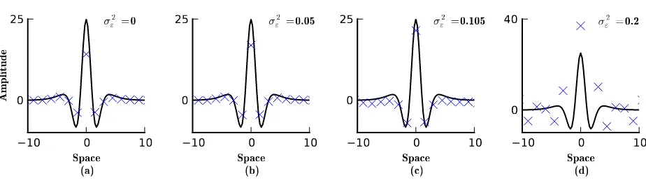
Next we studied the robustness of the estimator with errors in the assumed value of the observation

noise, where we estimated the spatial mixing kernel using different values ofσ2

are illustrated in Fig. 3. The Figure shows that the general shape of the mixing kernel can be recovered with

errors in the assumed value, provided the bound is satisfied. When the bound is not satisfied, the estimated

spatial mixing kernel is heavily distorted.

4.2. Example II: Anisotropic Mixing Kernels

In this section, we present results showing that the method can reliably recover anisotropic mixing

kernels from measured data. Estimation performance is illustrated with using two scenarios. It is worth

noting that recovering anisotropic mixing kernels is a problem that has previously been difficult to solve.

The difficulties are caused by the higher number of unknown parameters (with basis function placement)

when using anisotropic spatial mixing kernels in existing parametric methods. Due to our non-parametric

approach, issues with anisotropy are overcome.

For the first scenario the spatial mixing kernel is constructed from two basis functions that are offset

from the origin, leading to anisotropy. The kernel shown in Fig. 4(a). The parameters wereµ0 = [−0.5 0]

andµ1= [0 0.5], with amplitudes θ0= 100 and θ1=−100 and both widths set to 5.76.

The estimated kernel is depicted in Fig. 4(b). Cross-sections of actual and estimated kernels are shown

in Fig. 4(c). The Figures clearly show that the reconstructed spatial mixing kernel is in good accordance

with the actual kernel. The cross-sections of the actual and the estimated disturbance covariance functions

are also shown in Fig. 4(d), which also shows good concordance.

For the second scenario, a more complicated anisotropic mixing kernel is used. This time, the kernel is

constructed from four basis functions, where the centers are placed atµ0=µ1=µ2=0and µ3= [−3 0],

with widthsσ2

0= 3.24,σ12= 5.76,σ22= 36,σ32= 4, and amplitudesθ0= 80,θ1=−80,θ2= 5 andθ3= 15.

The resultant kernel is shown in Fig. 5(a). The estimated kernel is depicted in Fig. 5(b) with its cross-section

in Fig. 5(c). The cross-sections of the true and the estimated disturbance covariance functions are presented

in Fig. 5(d). The results show that the more complicated spatial mixing kernel and disturbance covariance

can be recovered by the new methods.

5. Conclusion

A novel and efficient approach for creating data-driven models of spatiotemporal systems has been

presented. We have presented a derivation of an estimator that can identify the spatial mixing kernel,

solutions, which extends linear systems theory to a broader class of spatiotemporal systems. The

closed-form solutions enable straight forward application of the theory, which will facilitates the identification and

modeling of a systems using the IDE framework.

Previous methods for identifying spatiotemporal properties of the IDE have involved more complicated

iterative algorithms [17, 18]. The complicated nature of the previous algorithms have potentially limited their

application in the general scientific domain, beyond the signal processing community. The IDE describes

a wide range of dynamical systems, including models of dispersion (where the shape of the kernel governs

the speed) and meteorological systems [1, 20]. Therefore, the new methods can potentially impact a wide

range of fields in scientific and engineering endeavor. Perhaps one of the most famous applications of the

IDE is with the Wilson and Cowan or Amari neural field model of the neocortex [33, 34]. In the Amari

neural field model (and many others), the spatial mixing kernel represents the neural connectivity function

and the disturbance covariance represents the receptive field for subcortical input [35, 36].

The analytic solutions in this paper can also be used to enhance existing methods for estimating and

tracking the dynamics of the field. For example, the closed-form solution for the estimated kernel can be

used to initialize the state-space EM algorithm framework of [17]. In fact, the solutions presented in this

paper should be a prerequisite for the EM algorithm. Previously, in state-space schemes the spatial mixing

kernel was recovered by inferring coefficients to basis functions. Until now, no good method existed for the

placement of kernel basis functions. Furthermore, the new methods presented in this paper will enhance

existing methods for tracking the dynamics of the field to overcome issues associated with anisotropy in the

mixing kernels. The estimated support of the disturbance covariance function also facilitates the application

of the EM algorithm for estimating the temporal variance in the disturbance signal. This way the disturbance

covariance matrix can be decomposed into two parts: an unknown scalar and a constant matrix depending

only on the inferred spatial support. Once the spatial support is estimated, recovering the disturbance

covariance matrix breaks down to the estimation of a single scalar parameter, improving the accuracy and

the convergence property of the algorithm.

The analytic solutions that we present in this paper are exact for a stationary system, that has an

infinite number of (temporal) samples that are acquired from an infinite number of sensors. Naturally, the

estimates of the spatial properties of the system will be approximate in any practical setting. Here we take

the opportunity to point out some issues regarding modeling choices. Firstly, care should be taken in dealing

with finite size effects. If the number of sensors is low, then there is the potential for significant errors to

kernel. Homogeneity is a restrictive assumption that limits the applicability of the model to systems where

the kernel is spatially invariant. If systems require a heterogeneous spatial mixing kernel, then alternative

modeling choices should be used such as [20]. Alternatively, one may use a spatiotemporal autoregressive

model. Modeling choices are often a trade-off between modeling accuracy or complexity, and the ability to

perform inference. The estimator that was derived in this paper is useful when efficiency out-weighs the

benefits of modeling heterogeneities. Finally, the accurate reconstruction of the spatial characteristics of

the IDE model requires making assumptions regarding the nature of the process and measurement noise.

These assumptions are standard and are necessarily to derive solutions and create useful tools [31, 15].

Nevertheless, care should be taken with quantifying and dealing with uncertainty. Future work should

investigate confidence bounds on the estimates.

The importance of spatiotemporal modeling is increasing with advances in technology as larger, higher

resolution datasets are being acquired. This research represents progress in modeling spatiotemporal

dy-namics, particularly with dealing with anisotropies and deriving an efficient estimator. Similar results have

previously existed for models that do not have spatial components, but these results have been overlooked

in spatiotemporal systems due to the added complexity in dealing with higher dimensions. The results

presented here pave the way and motivate further research to generalize and broaden the scope. Looking

forward, efforts should be directed towards incorporating heterogeneity into the spatial mixing kernels.

6. Acknowledgements

The research reported herein was partly supported by the Australian Research Council (LP100200571).

Dr Freestone acknowledges the support of the Australian American Fulbright Commission. The authors

also acknowledge valuable support and feedback from Prof Liam Paninski, Prof David Grayden, and Prof

[1] M. Kot, M. A. Lewis, P. van den Driessche, Dispersal data and the spread of invading organisms, Ecology 77 (7) (1996)

2027–2042.

[2] X. Zhou, X. Li, Dynamic spatio-temporal modeling for example-based human silhouette recovery, Signal Processing.

[3] Q. Zhang, Y. Chen, L. Wang, Multisensor video fusion based on spatial–temporal salience detection, Signal Processing

93 (9) (2013) 2485–2499.

[4] F. Amor, D. Rudrauf, V. Navarro, K. Ndiaye, L. Garnero, J. Martinerie, M. Le Van Quyen, Imaging brain synchrony

at high spatio-temporal resolution: application to MEG signals during absence seizures, Signal processing 85 (11) (2005)

2101–2111.

[5] A. Hegde, D. Erdogmus, D. S. Shiau, J. C. Principe, C. J. Sackellares, Quantifying spatio-temporal dependencies in

epileptic ECoG, Signal processing 85 (11) (2005) 2082–2100.

[6] S. Wolfram, Cellular Automata and Complexity, New York: Addison-Wesley, 1994.

[7] J. Wu, Theory and applications of partial functional differential equations, Vol. 119, Springer, 1996.

[8] B. Datsko, V. Gafiychuk, Chaotic dynamics in Bonhoffer–van der Pol fractional reaction–diffusion systems, Signal

Pro-cessing 91 (3) (2011) 452–460.

[9] S. Chow, J. Mallet-Paret, Pattern formation and spatial chaos in lattice dynamical systems. I, Circuits and Systems I:

Fundamental Theory and Applications, IEEE Transactions on 42 (10) (1995) 746–751.

[10] S. A. Billings, D. Coca, Identification of coupled map lattice models of deterministic distributed parameter systems, Int

J Syst. Sci. 33 (8) (2002) 623–634.

[11] L. Lin, M. Shen, H. C. So, C. Chang, Convergence analysis for initial condition estimation in coupled map lattice systems,

Signal Processing, IEEE Transactions on 60 (8) (2012) 4426–4432.

[12] P. E. Pfeifer, S. J. Deutsch, Identification and interpretation of first order space-time ARMA models, Technometrics 22 (3)

(1980) 397–408.

[13] M. Dewar, V. Kadirkamanathan, A canonical space-time state space model: State and parameter estimation, Signal

Processing, IEEE Transactions on 55 (10) (2007) 4862–4870.

[14] P. Aram, V. Kadirkamanathan, S. Anderson, Spatiotemporal system identification with continuous spatial maps and

sparse estimation., Neural Networks and Learning Systems, IEEE Transactions on.

[15] N. Cressie, C. K. Wikle, Statistics for spatio-temporal data, Vol. 465, Wiley, 2011.

[16] S. A. Billings, Nonlinear system identification: NARMAX methods in the time, frequency, and spatio-temporal domains,

John Wiley & Sons, 2013.

[17] M. Dewar, K. Scerri, V. Kadirkamanathan, Data-driven spatio-temporal modeling using the integro-difference equation,

Signal Processing, IEEE Transactions on 57 (1) (2009) 83–91.

[18] K. Scerri, M. Dewar, V. Kadirkamanathan, Estimation and Model Selection for an IDE-Based Spatio-Temporal Model,

Signal Processing, IEEE Transactions on 57 (2) (2009) 482–492.

[19] C. Wikle, N. Cressie, A dimension-reduced approach to space-time kalman filtering, Biometrika 86 (4) (1999) 815–829.

[20] K. Xu, W. C. K, F. Neil, A kernel-based spatio-temporal dynamical model for nowcasting weather radar reflectivities,

Journal of the American Statistical Association 100 (472) (2005) 1133–1144.

[21] C. K. Wikle, S. Holan, Polynomial nonlinear spatio-temporal integro-difference equation models, Journal of Time Series

Analysis.

[23] M. A. Figueiredo, A. K. Jain, Unsupervised learning of finite mixture models, Pattern Analysis and Machine Intelligence,

IEEE Transactions on 24 (3) (2002) 381–396.

[24] G. Biagetti, P. Crippa, A. Curzi, C. Turchetti, Unsupervised identification of nonstationary dynamical systems using a

gaussian mixture model based on em clustering of soms, in: Circuits and Systems (ISCAS), Proceedings of 2010 IEEE

International Symposium on, IEEE, 2010, pp. 3509–3512.

[25] P. Eykhoff, System Identification: Parameter and State Estimation, Wiley, 1974.

[26] L. Ljung, System identification: theory for the user, Prentice-Hall Information and System Sciences Series, Englewood

Cliffs, NJ., 1987.

[27] J. S. Bendat, A. G. Piersol, Random data: analysis and measurement procedures, Vol. 729, John Wiley & Sons, 2011.

[28] R. Pintelon, J. Schoukens, System identification: a frequency domain approach, John Wiley & Sons, 2012.

[29] C. Rasmussen, C. Williams, Gaussian Processes for Machine Learning (Adaptive Computation and Machine Learning),

The MIT Press, Cambridge MA, 2005.

[30] D. Ricker, Echo signal processing, Springer Netherlands, 2003.

[31] L. Ljung, T. S¨oderstr¨om, Theory and practice of recursive identification, MIT Press, Cambridge, MA, 1983.

[32] L. Ljung, Characterization of the concept of ‘persistently exciting’ in the frequency domains, Lund Inst. of Technology,

Division of Automatic Control, 1971.

[33] H. Wilson, J. Cowan, A mathematical theory of the functional dynamics of cortical and thalamic nervous tissue, Biological

Cybernetics 13 (2) (1973) 55–80.

[34] S. Amari, Dynamics of pattern formation in lateral-inhibition type neural fields, Biological Cybernetics 27 (2) (1977)

77–87.

[35] D. R. Freestone, P. Aram, M. Dewar, K. Scerri, D. B. Grayden, V. Kadirkamanathan, A data-driven framework for neural

field modeling, NeuroImage 56 (3) (2011) 1043–1058.

[36] P. Aram, D. Freestone, M. Dewar, K. Scerri, V. Jirsa, D. Grayden, V. Kadirkamanathan, Spatiotemporal multi-resolution

−30 0 30 −30

0 30

−0.8

0.0 0.6

10 0 10

Space

(a)

0 10

Space

10 0 10

Space

(b)

0 10

10 0 10 20

10 0 10

Space

(c)

0 25

Amplitude

κ(

r

r

10 0 10

Space

(d)

0 0.12

η(

r

r

10 0 10

Space

(a)

0 25

Amplitude

σ2 ε =

0

10 0 10

Space

(b)

0

25 σ2

ε =

0.05

10 0 10

Space

(c)

0

25 σ2

ε =

0.105

10 0 10

Space

(d)

0

40 σ2

ε =

0.2

10 0 10

Space

(a)

0 10

Space

10 0 10

Space

(b)

0 10

20 0 25

10 0 10

Space

(c)

20 0 25

Amplitude

κ(

r

r

10 0 10

Space

(d)

0 0.12

η(

r

r

10 0 10

Space

(a)

0 10

Space

10 0 10

Space

(b)

0 10

10 0 10

10 0 10

Space

(c)

10 0 10

Amplitude

κ(

r

r

10 0 10

Space

(d)

0 0.12

η(

r

r