A Physically-based, Subgrid Parametrization for the Production and Maintenance of Mixed-phase Clouds in a General Circulation Model

This is a repository copy of

A Physically-based, Subgrid Parametrization for the Production

and Maintenance of Mixed-phase Clouds in a General Circulation Model

.

White Rose Research Online URL for this paper:

http://eprints.whiterose.ac.uk/91977/

Version: Published Version

Article:

Furtado, K, Field, PR, Boutle, IA et al. (2 more authors) (2016) A Physically-based, Subgrid

Parametrization for the Production and Maintenance of Mixed-phase Clouds in a General

Circulation Model. Journal of the Atmospheric Sciences, 73 (1). pp. 279-291. ISSN

0022-4928

https://doi.org/10.1175/JAS-D-15-0021.1

[email protected] https://eprints.whiterose.ac.uk/

Reuse

Unless indicated otherwise, fulltext items are protected by copyright with all rights reserved. The copyright exception in section 29 of the Copyright, Designs and Patents Act 1988 allows the making of a single copy solely for the purpose of non-commercial research or private study within the limits of fair dealing. The publisher or other rights-holder may allow further reproduction and re-use of this version - refer to the White Rose Research Online record for this item. Where records identify the publisher as the copyright holder, users can verify any specific terms of use on the publisher’s website.

Takedown

If you consider content in White Rose Research Online to be in breach of UK law, please notify us by

A Physically Based Subgrid Parameterization for the Production and Maintenance

of Mixed-Phase Clouds in a General Circulation Model

K. FURTADO, P. R. FIELD, I. A. BOUTLE, C. J. MORCRETTE,ANDJ. M. WILKINSON

Met Office, Exeter, United Kingdom

(Manuscript received 15 January 2015, in final form 10 September 2015)

ABSTRACT

A physically based method for parameterizing the role of subgrid-scale turbulence in the production and maintenance of supercooled liquid water and mixed-phase clouds is presented. The approach used is to simplify the dynamics of supersaturation fluctuations to a stochastic differential equation that can be solved analytically, giving increments to the prognostic liquid cloud fraction and liquid water content fields in a general circulation model (GCM). Elsewhere, it has been demonstrated that the approach captures the properties of decameter-resolution large-eddy simulations of a turbulent mixed-phase environment. In this paper, it is shown that it can be implemented in a GCM, and the effects that this has on Southern Ocean biases and on Arctic stratus are investigated.

1. Introduction

Mixed-phase and supercooled liquid water clouds are known to be difficult to represent in numerical weather prediction (NWP) and climate models. This has been implicated as a potential cause of serious model biases. For example, many of the IPCC models exhibit large sea surface temperature biases over the Southern Ocean. This adversely effects the global cir-culation and leads to difficulties in simulations of the cryosphere, such as underestimation of the extent of Antarctic sea ice. Given the critical role of the South-ern Ocean for energy and carbon uptake, deep-water mass formation, and climate sensitivity, alleviation of these biases is seen as a priority for climate prediction (Rintoul 2011). Southern Ocean surface temperature biases are accompanied by a bias in the shortwave (SW) radiation reflected to space by clouds (Bodas-Salcedo et al. 2014), the most likely cause of which is insufficient amounts of model supercooled liquid water.

Similar problems have been identified in the simula-tion of Arctic climates. In a study of Arctic stratus clouds, Klein et al. (2009) showed that many models have significant surface radiation biases that are linked to the determination of the phase of the condensate.

Hypotheses exist for why models struggle to represent mixed-phase clouds [seeKlein et al. (2009)for a review]. For example,Forbes and Ahlgrimm (2014)incorporated the subgrid vertical structure of mixed-phase clouds into a general circulation model (GCM) by making microphys-ical process rates depend directly on the distance from cloud top. Another suggestion (e.g., Korolev and Field 2008) is that small-scale turbulence plays a role by driving fluctuations in relative humidity that lead to the conden-sation of liquid water. In competition with this effect is the depositional sink of water vapor to the ice phase, which acts to damp out humidity fluctuations. If real-world mixed-phase clouds owe their longevity to the interplay of these processes, then their accurate parameterization in numerical models becomes important because, as a result of computational constraints, GCMs cannot resolve small-scale variability. Indeed, at climate model resolutions, subgrid humidity variability (due to unresolved eddying motions) must ultimately account for the majority of liq-uid water formation, and it is the long-recognized goal of GCM cloud schemes to parameterize this condensation pathway in terms of the resolved model variables.

In this paper, we will consider how turbulence forms and maintains mixed-phase clouds and propose a method for including these effects in numerical models. Our ap-proach originates in the study byField et al. (2014, here-after F14), who proposed an analytically soluble model of mixed-phase cloud dynamics based on a stochastic dif-ferential equation for supersaturation fluctuations. Their Corresponding author address: Kalli Furtado, Met Office, FitzRoy

Rd., Exeter EX1 3PB, United Kingdom. E-mail: [email protected]

model gave the liquid cloud properties in terms of the local turbulence and the properties of any preexisting ice cloud and agreed well with the results of decameter-scale large-eddy simulations.

Broadly speaking,F14sought to address the following question: given the turbulent and ice microphysical state of a preexisting ice cloud, can the liquid phase properties be determined analytically from the underlying dy-namical equations? Although their approach was ini-tially used to analyze mixed-phase environments, it naturally contains the ice-free limit as a special case and can therefore be applied to predict liquid condensation from clear-sky conditions at any temperature.

To describe the turbulence,F14used the turbulent ki-netic energy (TKE) and dissipation rate. They also ac-counted for mixing of environmental air into cloudy regions, modeled via the mixing length over which turbu-lent transport occurred. Ice effects were included via the phase-relaxation time scale, characterizing the rate at which the conditions in a fluid parcel attain ice saturation. It was shown that the above parameters completely specify the steady-state probability density function (PDF) of su-persaturation fluctuations inside an air volume. This PDF can then be inspected to obtain the liquid cloud properties, which appear naturally as truncated PDF moments.

In this paper, we will use theF14method to develop a parameterization of subgrid liquid water cloud pro-duction for use in a GCM. In each model grid box, the analytical solution ofF14will be applied to diagnose the liquid cloud properties from the gridbox-mean vari-ables. Closure relations will be introduced to obtain the turbulence information needed to determine the subgrid statistics. The effect of the parameterization on South-ern Ocean radiative biases and simulations of Arctic stratus clouds will then be considered.

2. Model description and implementation

The starting point for the study byF14is a modified form of the linearized Squires equation for the super-saturationSiwith respect to ice:

dS_i dt 5 2

S_i t_p2

S_i2S_E

t_E 1aiw, (1)

whered/dt is the Lagrangian time derivative,w is the turbulent vertical velocity, tp is the phase-relaxation time scale,SEis the environmental supersaturation with

respect to ice, tE is a mixing time scale, and ai is a

function of temperature (see theappendix).

The standard version of Squires equation is obtained from Eq. (1) by omitting the term (SE2Si)/tE. F14

added this term to model the exchange of air parcels

between a turbulent zone of depth‘_{Eand its} surround-ings. The time needed for homogenization by turbulent diffusion over this length scale is given by

t_E5

_‘2

E

1/3

, (2)

where_{is the turbulent dissipation rate.}

To include the effects of turbulence,F14modeledwas Gaussian white noise with variances2

wand autocorrelation

hw(t₁)w(t₂)i5s2_wt_dd(t₁2t₂) , (3)

wheredis the Dirac distribution, andtdis the Lagrangian

decorrelation time scale, characterizing vertical velocity correlations along fluid parcel trajectories. Throughout this paper, we will use angle brackets to denote ensemble averages over realizations ofw.

For homogeneous, isotropic, stationary turbulence, it is known that

t_d52s 2

w

_C

0

, (4)

whereC0is an empirical constant (Rodean 1997).

The effects of ice enter via the phase relaxation time scale, which is defined by

t_p5 1

b_iB₀M₁, (5)

where M1 is the first moment of the ice particle size

distribution, andbiandB0are functions of temperature

given in theappendix.

Equation(1)can be solved analytically for the statistics ofSi. In particular, it can be shown that the steady-state PDFF(Si) ofSiis Gaussian with variances2

S and mean hSii, given by

s2_S5(1/2)a 2

is

2

wtd

1/t_p11/t_E and (6)

hS_ii5S_E 1/tE

1/t_p11/t_E. (7)

The liquid cloud fraction f and mean liquid water mass mixing ratiohqliare given by the following trun-cated moments of theSiPDF:

f5

ð‘

S_iw

ds F(s) and (8)

hq_li5

ð‘

S_iw

whereSiwis the value of the ice supersaturation in

water-saturated conditions, andqsiis the saturated mass

mix-ing ratio of water vapor in air with respect to ice. We note that the integrals in Eqs.(8)and(9) can be per-formed analytically.

a. Underlying assumptions

In this section, we revisit the derivation of the F14

model to highlight the assumptions on which it is based. The premise of the model is that the cloud liquid water content can be deduced by inspecting the PDF of ice supersaturation in the absence of liquid condensate. However, we propose that it can also be used to repre-sent the supersaturation dynamics once an air parcel becomes mixed phase.

Diagnosing liquid cloud properties from the PDF ofSi

is possible because of the dynamical equivalence between the water vapor mixing ratioqyin a system without liquid

water andqy1qlin a system that includes a massqlof

liquid water per unit mass of dry air. To make this more precise, let us define the liquid water supersaturation with respect to iceh_ito be

h_i5 qy1ql

q_si(p,T_l)21 , (10)

whereTl5T2Lyql/cp is the liquid water temperature

of the system, andTandpare the air temperature and pressure.

It can be shown that, for temperatures below 08C, the dynamical equation forh_ican be obtained from Eq.(1)by substitutingh_i in place ofSi. In other words,h_ievolves according to the same equation as doesSiin the absence of liquid water. Hence, the results ofF14can be interpreted as giving analytical expressions for the PDF ofhi.

Note that forT.08C, we can modify the definition ofhi

by replacingqsi with its liquid water counterpartqsw.

Dy-namically, the resultant quantity is still equivalent toSiifLy

is substituted forLsin the definitions ofai,bi, andB0. F14comparedSiwithSiwto determine the threshold

for liquid water condensation. However, the exact cri-terion for condensation of liquid water is

h_i.qsw(p,T)

q_si(p,T_l)21 , (11)

which necessarily involvesqlvia the liquid water

tem-perature. This induces an inconvenient circularity: one cannot diagnose the presence of liquid water without already knowing the value ofql.

However, the right-hand side of inequality (11) is approximatelySiw(p,T) ifql is sufficiently small. This suggests that the model ofF14applies only in situations

where latent heating due to liquid condensation can be neglected. This is equivalent to introducing the follow-ing approximation:

a_iLy c_pql5

L_yL_sq_l

c_pR_yT21 , (12)

whereai5›lnqsi/›T (see theappendixfor a complete nomenclature of symbols); that is, the fractional change inqsidue to latent heating is small. We will call condition

(12) the small ql approximation.Figure 1gives an in-dication as to its range of validity. The parameterization implemented here is most active for temperatures warmer than 2158C and typically gives condensation increments in the range 0.1–0.5 g kg21

. FromFig. 1, this corresponds to errors of around 10%; however, this is lower (e.g., 5%) for cold clouds.

We can then identify the subset of phase space that corresponds to nonzeroqlas approximately those points

for which

h_i.S_iw(p,hTi) , (13)

where we have made the further assumption thatTcan be replaced with its mean value hTi. [Note that, for temperature fluctuations on the order ofLyhqli/cp, this

follows from Eq.(12).]

Furthermore, the amount of liquid water present at any one of these phase points is

q_l5q_si(p,hTi)[h_i2S_iw(p,hTi)] . (14)

Condition(13)and Eq.(14)correspond to the model of F14 for temperature below 08C. For temperatures above 08C, Eqs.(13)and(14)continue to hold, provided one substitutesqswforqsi, thereby settingSiw50.

In this paper, we interpret theF14 model as giving PDFs of the humidity variable hi. The above small ql

approximation can then be used to predict mean liquid water mass mixing ratio hqli and cloud fraction f. As

inputs, the model requires the parameters needed to specify theh_iPDF, along with the valuespandhTi.

b. Closure relations

To implement the model in a GCM, closure relations are required for the parameters that determine the su-persaturation distribution in each model grid box. We re-call that the following variables are required: the vertical velocity variances2_w, the eddy dissipation rate_{, the} tur-bulent mixing length‘_{E, the turbulent decorrelation time} scaletd, and the supersaturationSE of the air entrained

from the surroundings. In addition, we must specify the mean values ofpandTfor the state of the subgrid model. These latter two quantities we will take to be equal to the resolved values in the grid box:hTi5Tandp5p. We use an overbar for gridbox-mean quantities.

Consistency between the closure relations requires that Eq.(4)hold fortd. In addition, we choose to impose

the constraint that

‘

E5tdsw. (15)

This equation states that the turbulent mixing length is the typical decorrelation length scale of the unresolved eddies.

In the Met Office Unified Model,s2_wis a diagnostic from the boundary layer scheme, although it is avail-able at all altitudes. In regions wheres2_wis small, the subgrid PDF is very narrow, and no liquid water is produced. The scheme is therefore able to produce liquid cloud at any altitude where sufficient turbulence is diagnosed, although in practice its effects are largest in the boundary layer wheres2

wis large. By

construc-tion, the TKE diagnostic is zero in regions of deep convection.

We impose the constraint that the unresolved mo-tions are similar in vertical extent to the gridbox depth

Dz. Hence, the mixing length‘E5b1Dz, whereb1 is a

proportionality constant. We will takeb1to be an

ad-justable tuning parameter, subject to the constraint that it should be of order 1. In physical terms, we therefore have in mind an ensemble of subgrid-scale motions (eddies), each driven by an independent random re-alization of the subgrid noisewand making excursions that are on the order of gridbox depth. In this paper, we chooseb152.

Using Eqs.(2)and(4)and the eddy size constraint equation [Eq.(15)], we obtain closed expressions for

tdandtE:

t_d5b1Dz

s_w 5b2tE, (16)

whereb25(2/C0)1/3. FollowingF14, we will setC0510

[Rodean (1997)states that estimates are in the range 0.6–10; seeF14for a detailed discussion]. Using Eq.(16), we can diagnose the dissipation rate_{from Eq.(4).}

The phase-relaxation time scaletpis calculated using Eq.(5)with the gridbox-mean valuesT andpand first moment of ice particle size distribution M1 from the

cloud microphysics scheme. The environmental super-saturation SE is assumed to be the gridbox-mean

su-persaturation Si. We note that the turbulent cloud production scheme does not change the amount of ice in a grid box: rather, it uses information about preex-isting ice to determine how much liquid water conden-sation occurs. The growth of ice from vapor occurs only in a cloud microphysics scheme. Hence, although this condensation mechanism and the cloud microphysics scheme both deplete qy, this depletion represents

dif-ferent processes in the two schemes.

Using these closures in Eqs.(6)and(7)gives the fol-lowing expressions fors2_SandhSii:

s2_S5 (1/2)a 2

ib1swDz b_iB₀M₁1gs_w/Dz

and (17)

hS_ii5 gswSi/Dz b_iB₀M₁1gs_w/Dz

. (18)

where it is convenient to define a constantg5b2/b1.

Two limiting cases are of interest:

(i) Microphysics dominated:tptE.In this case,sS

and hSii tend to zero. In the presence of large amounts of ice, the supersaturation distribution becomes very sharply peaked around ice saturation. (ii) Entrainment dominated:tEtp. In this case,

s_S;a_iD_z,hS_ii;S_i. (19)

In the presence of rapid entrainment from the environ-ment, the cloud layer quickly homogenizes to the hu-midity of the environment, and the supersaturation fluctuations are determined by the vertical extent of the turbulent excursions.

c. Incrementing model prognostics

The most prosaic way of implementing the scheme is to use the values calculated from Eqs.(8) and(9) to increment the GCM prognostics for ql,qy,T, and f.

For example, if the turbulent cloud production pa-rameterization diagnoses a liquid water content hqli

ql, then the resultant increment to the gridbox-mean

value is

Dq_l5hq_li2q_l, (20)

together with a compensating change in the water vapor prognostic and an amount of latent heatingLyDql/cp.

However, applying the same recipe to cloud fraction increments leads to the following inconsistency with the GCM macroscale cloud scheme.

Underlying the Unified Model macroscale cloud scheme [prognostic cloud fraction and prognostic condensate (PC2) scheme;Wilson et al. 2008] is an implicit PDF for subgrid moisture variability. To initialize the liquid cloud fields away from states with zero cloud fraction, the PC2 scheme uses a diagnosed PDF width based on the vertical profile of an adjustable parameter: the crit-ical relative humidity (RHc). This diagnosed profile

represents the PDF widths at the onset of cloud for-mation. An equivalent approach is used to initialize the liquid cloud fields away from totally overcast states by breaking up overcast skies when the gridbox-mean total relative humidity falls below 22RHc.

Care must therefore be taken with any parameteriza-tion that can add significant amounts of cloud fracparameteriza-tion to the model. Suppose a parameterization elevates the cloud fraction tof51 in a grid box that is then diagnosed by the PC2 scheme to meet the criteria for initialization away from overcast skies. The PC2 initialization param-eterization will then remove some of the additional cloud fraction, almost immediately counteracting the desired tendency toward greater cloudiness.

This situation essentially arises because the turbulent production parameterization and the PC2 initialization scheme have conflicting definitions of the critical rela-tive humidity. We must therefore adopt a method that calculatesf increments that are consistent with both the turbulence-based scheme and the underlying PC2 cloud scheme.

One such method is the following. The increments toql

are determined by the turbulent production mechanism [i.e., from Eq.(9)] using the recipe given above. The cloud fraction increment, however, is not found from Eq.(8). Instead, we use available resolved-scale information to determine afincrement that is consistent with the cur-rent state of moisture PDF from the PC2 cloud scheme. To do this, we use the fact that, as shown inMorcrette (2012), changes infandqlcan be related by

Df5QcG(2Qc)

fQ_c2q_l Dql, (21)

whereGis the subgrid moisture PDF in the macro-scale cloud scheme, andQcis the boundary between

the saturated and unsaturated parts of the moisture PDF.

The f increments determined in this way will be consistent with the underlying subgrid variability that is implicit in the PC2 cloud scheme [via the parameteri-zation ofG(2Qc)]. As a consequence, the RHc-based,

PC2 initiation scheme is inhibited from counteracting the turbulence-driven scheme. In addition, we note that the structure of the PC2 code prevents PC2 initiation from initializing more cloud in grid boxes that already contain liquid water. Hence, in the regions with signifi-cant TKE, the turbulent production scheme overrides PC2 initiation as the main condensation pathway.

Figure 2ashows a typical globals2_w field from a low-resolution global model a couple of hours into the simu-lation at a height of 1 km.Figures 2b and 2cshow the as-sociated increments ofql andf. It can be seen that the

liquid cloud increments are located in the turbulent re-gions. More intense turbulence tends to imply larger cloud increments. However regions of highs2

wwith little liquid

cloud produced can also be identified. This occurs when the gridbox-mean state is too dry for the parameterized subgrid motions to produce liquid water (e.g., over Australia).

Note that, inFigs. 2b and 2c, orange is used to denote grid boxes where the cloud increments are below the lower limit of the color scale. Hence, inFig. 2b, orange regions show the (relatively infrequent) occurrence of negativeqlincrements. This happens where the scheme diagnoses less liquid condensate than is already present in the model grid box. Similarly, inFig. 2c, orange de-notes regions where the cloud fraction decreases as a result of the scheme. This occurs because, as noted in

Wilson et al. (2008), Eq.(21)does not constrainDfto be positive for positiveDqlif the grid box is moist enough.

Typically, however, we have found Df to be small (greater than20.05) when negative.

3. NWP simulations

a. Comparison to AMSR

described by D. N. Walters et al. (2015, unpublished manuscript). We test the effect of adding the turbulent cloud production parameterization to this model. To de-termine the model liquid water paths, we sum contribu-tions from the model large-scale (stratiform) cloud and convection schemes.1

AMSR-E provides cloud water path and surface rain rate products that are interrelated by the algorithm de-scribed in Hilburn and Wentz (2008). If a drop size distribution and fall speed–size relation are assumed for rain, then the algorithm can be inverted to obtain an estimate of the total liquid water path (LWP). Here, we have assumed the fall speed relation according to

Sachidananda and Zrnic (1986) and the particle size distribution fromAbel and Boutle (2012).

Figure 3acompares the zonal- and time-averaged AMSR-E liquid water path (red line) to the model pre-dictions. The line-filled regions show the envelopes of zonally averaged model LWP. AMSR observations are not available over land or sea ice, and the model has therefore been filtered to correspond with the AMSR data mask.

South of 508S and in the Arctic, the control model (black-lined region) underpredicts the LWP. Including the turbulent production parameterization (green-lined region) increases the LWPs and goes some way to ad-dressing this bias. Note that the latitudinal coverage of the comparison is limited by the extent of the polar sea ice. In the tropics and subtropics, however, the experi-ment overpredicts the LWP. In fact, away from the polar regions, the control model agrees reasonably well with the observations.

Only the model large-scale cloud-scheme LWP is di-rectly affected by the turbulent production mechanism.

Figure 3bshows that the parameterization increases the model large-scale LWP by approximately 50%.

Increasing the stratiform cloud LWP will cause more SW radiation to be reflected back to space. Over the Southern Ocean, this effect is beneficial because the Unified Model has a large negative bias in outgoing SW radiation in that region (Bodas-Salcedo et al. 2014). Similarly, the increase in Arctic LWP will enhance the surface downwelling longwave (LW) flux, which is also negatively biased in the control model.

The extra stratiform tropical and subtropical LWP is not beneficial and leads to a positive bias in reflected SW over the tropics. There are several possible reasons for FIG. 2. Instantaneous global fields at a height of 1120 m above

the surface, 2 h into an N96L70 (130-km horizontal grid spacing, 70 vertical levels) global simulation. (a) The variance of the tur-bulent vertical velocity, diagnosed by the boundary layer scheme; (b) liquid water mass mixing ratio increment produced by the scheme; and (c) liquid cloud fraction increment produced by the scheme.

1_{The convective cloud water content is derived as a product of}

this. First, there may be flaws in the parameterization, either because of simplifications in theF14model itself, or because of the closure relations used in this im-plementation. Second, there are uncertainties in the way in which liquid water paths are estimated from the model convection scheme and the AMSR surface rain rates. In addition, other sources of model error may be complicating the comparisons. For example, the model may contain too much rainwater.

Third, it is known that the control model possesses a good representation of subtropical/tropical cloud compared with other models (Wyant et al. 2010). Parameterizing a previously unrepresented pathway to cloud formation, as has been done here, may therefore be likely to degrade the model for warm clouds simply because the model is already in a rela-tively acceptable state. This would suggest that

weaknesses in warm clouds could be remedied by tuning parameterizations as part of a much broader model development activity.

By contrast, for cold clouds, the control model is sub-optimal with respect to cloud phase, as evidenced byFig. 3

and the large Southern Ocean radiative biases. This is be-cause existing PC2 processes are not providing a significant source of liquid water within cold clouds. We argue that this is precisely because they do not represent the main pathway to cold-cloud formation: namely, inhomogeneous conden-sation in response to small-scale turbulent fluctuations.2 Hence, by adding this process, there is considerable scope to improve the representation of cold clouds.

Finally, perhaps the scheme leads to processes being overparameterized, in the sense of their being handled by two separate parameterizations. This, however, should not be the case. The method described insection 2cprevents any inconsistency with the PC2 initiation parameterization (which does not act if the turbulence-based scheme has done so). In addition, there should be no overlap of phys-ical processes between the current scheme and other PC2 source terms, since the latter either are homogeneous forcings in response to spatially uniform cooling or hu-midification, without change to the underlying PDF shape (e.g., boundary layer scheme increments) or are caused by manifestly different physics (e.g., convective detrainment). In summary, we are left with a need for a pragmatic way of retaining the benefit of more LWP at high latitudes, but without the detrimental effects in the subtropics. To this end, we choose to implement the turbulent cloud pro-duction mechanism only in grid boxes where the tem-perature is below 08C. We revisit this issue in the context of climate simulation insection 4.

b. M-PACE simulations

We consider the effect of the turbulent cloud production parameterization on NWP simulations of the Mixed-Phase Arctic Cloud Experiment (M-PACE) flying period (Klein et al. 2009). M-PACE was an aircraft campaign with co-incident ground-based measurements, which took place over Barrow in northern Alaska in October 2004. The observations show a stratiform mixed-phase cloud deck underlying a weak inversion at a height of around 1.5 km and descending to 0.5 km from the surface. In situ mea-surements showed the vertical profile of liquid water content increasing toward the cloud top, which had a typ-ical temperature of2158C. Below the mixed-phase layer, snowfall was recorded that extended down to the surface. FIG. 3. Comparison of model LWPs to AMSR-E. (a) Total LWP,

all cloud types. (b) Model large-scale (stratiform) cloud LWP (excluding large-scale rain and convective condensate). In (a), the red line shows the zonal and time average of the AMSR-E obser-vations for the 6-day period ending 24 Sep 2011. The line-filled envelopes show model LWP ranges for the same period for the control (black) and experiment (green) configurations. The vertical red bars show the range of AMSR-E observations.

2_{The only PC2 process that does try to represent this process is}

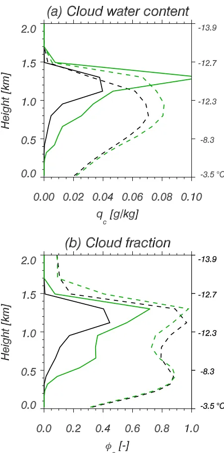
Figure 4shows the changes in the mean vertical liquid cloud profiles along a cross section through the target area. The transect chosen for the cross section joins the Barrow Atmospheric Radiation Measurement (ARM) Program site in the northwest to Oliktok Point, ap-proximately 300 km to the southeast, and corresponds

closely to the flight path of the aircraft during the ex-periment. The left-hand-side vertical axes inFig. 4show height above the surface. The profiles are means con-structed from hourly model outputs over a 12-h period beginning at 1700 UTC 9 October 2004. The model used is the N512 global model described insection 3a. Initial conditions were prescribed at 0000 UTC 9 October, using an ECMWF analysis.

Profiles from two model runs are plotted inFig. 4. The control model, shown by the black lines, is compared to an experiment that includes the turbulent cloud pro-duction parameterization. The solid lines show liquid water contents and cloud fractions; the dashed lines are for ice cloud.

The experiment shows significantly more liquid cloud throughout the depth of the profile. The profile of ql

becomes more adiabatic in character, with the biggest increases in liquid water content occurring near cloud top, where enhanced TKE due to cloud-top instability drives the production of extra liquid water.

The cloud-top liquid water contents attained are still much lower than those observed: 0.1 g kg21 in the ex-periment model compared with 0.3 g kg21_{in the}

obser-vations. In addition, the model ice water contents are larger than observed and typically exceed the liquid water contents. This problem is exacerbated in the experiment because of riming of the increased liquid water.

The improvements made to the subgrid cloud frac-tion fields are relatively modest. The observed stratus had mixed-phase cloud fractions of close to 1 throughout its depth (Klein et al. 2009). Figure 4b

shows that the liquid cloud fractions have increased in the experiment but remain significantly lower than were recorded in reality.

Figure 5shows the mean thermodynamic structure of the boundary layer in the two models. Also shown are the mean vertical extents of the cloud layers.3

The cloud base in the control model is typically too high, compared to the observed value of 500 m. The experiment shows more frequent occurrence of low cloud bases, and this improves the mean cloud-base forecast. The temperature range of cloud (also shown in

Fig. 4) is similar to that inferred from the observations [cf. Fig. 2 ofKlein et al. (2009)]. However, the coldest temperatures attained at the inversion are around a degree warmer than the reported cloud top of2158C. This is potentially due to underresolution of the in-version structure because of vertical grid spacing. FIG. 4. Vertical profiles of (a) gridbox-mean condensed water

content for liquid (solid lines) and ice (dashed lines), and (b) cloud fractionfcof liquid (solid lines) and ice (dashed lines) along a cross section through the target region, around Barrow on the North Slope of Alaska, for the two N512 global model forecasts. The fields are averaged along a transect joining 70.518N, 1498W and 71.38N, 1578W for a 12-h time interval. The black lines are for the control model, and the green lines are for the experiment.

3_{FollowingKlein et al. (2009), we define cloud base as the height}

For the Arctic climate, it is interesting to consider the effects of the additional liquid cloud on the surface ra-diation budget.Figure 6shows the joint PDF of surface downwelling LW flux and liquid water path. The statis-tics were obtained for a 1.28 38.88rectangle centered on 70.58N, 1538W, which includes the two ARM sites. The black contours show the joint PDF for the control model; the green contours show those for the experi-ment. The green and black symbols correspond to Bar-row and Oliktok Point, at both of which the liquid water paths more than doubled. The increase in LWP has a radiative impact at the surface, leading to an average increase in surface downwelling LW of approximately 10 W m22

and bringing the forecast closer to the obser-vations (shown by the gray rectangle). The variability of the model fields is also improved: the control model gives a longer tail of low LWPs and LW fluxes, which is shifted to higher values in the experiment. However, it is clear that deficiencies remain in the way the model represents Arctic stratus cloud.

4. Climate simulations

In this section, we consider the effects of the turbu-lent cloud production parameterization on 20-yr climate

simulations. In particular, we quantify the impact of the additional liquid cloud on the model top-of-atmosphere (TOA) and surface radiation biases. The control model used is similar to the GA6 con-figuration of the Met Office Unified Model at N96L70 resolution (approximate horizontal grid spacing is 130 km).

As shown insection 3a, applying the turbulent cloud production scheme for all temperatures results in a sig-nificant increase in large-scale cloud LWP globally. At high latitudes, this increase addresses an existing LWP deficit in the control model. However, the significant increase in tropical large-scale cloud due to the scheme leads to a very large increase in outgoing SW radiation over the tropics. Consequently, for the climate simula-tions presented here, we constrain the scheme to oper-ate only for temperatures below 08C. This effectively restricts the production of additional liquid cloud to the poles and midlatitudes. In future work, it may be pos-sible to relax this temperature restriction by making alterations to the model cloud and radiation schemes.

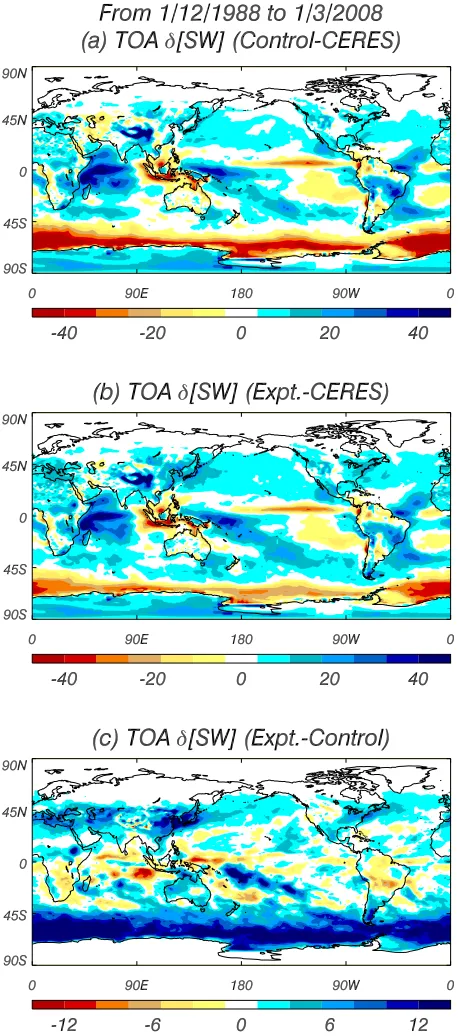
Figures 7a and 7bshow the 20-yr mean bias in TOA outgoing SW flux for the control and experiment, rela-tive to CERES-EBAF (Loeb et al. 2009) in the Southern Hemisphere summer. There is a very large negative shortwave bias over the Southern Ocean for the control model that is significantly reduced for the experiment. The extent of the bias reduction is apparent fromFig. 7c, FIG. 6. Joint histogram of surface downwelling longwave flux and LWP for the North Slope of Alaska region. The line-filled box shows the M-PACE observations. The small colored symbols show the means at Barrow (circles) and Oliktok Point (squares). FIG. 5. Vertical profiles of potential temperature (solid lines;

which shows the differences in the outgoing TOA shortwave flux between the two models.

Figure 8ashows the zonally averaged, 20-yr TOA flux differences. The additional liquid water produced at

midlatitudes in both hemispheres results in an increase in the reflected SW of up to 6 W m22and a decrease in outgoing LW of 2 W m22.

The effect on model TOA fluxes is similar in both hemispheres. This can also be seen fromFig. 7, where brightening of clouds is visible, for example, over the North Pacific and the Sea of Japan. Because Northern Hemisphere SW biases are smaller than those over the Southern Ocean, and typically positive in sign, bright-ening of Northern Hemisphere clouds is detrimental to the SW. This is most pronounced in the Arctic during the summer (not shown). However, given severity of the Southern Ocean biases and their importance for climate prediction, improvement there might be valued over degradation elsewhere.

Figure 8bshows the zonally averaged differences in the surface fluxes. The total surface flux is a sum of the net surface LW and SW fluxes, sensible heat flux, and latent heat flux. The black line shows how the total surface flux differs between the control and experiment. The effect of the increased liquid cloud in the experi-ment is to reduce the total energy flux into the surface over most of the regions that show increased cloudiness. Over the Southern Ocean, for example, the total energy flux is reduced in the experiment by up to 4 W m22_.

Also shown inFig. 8care the various contributions to the surface energy balance. The net flux of SW radia-tion into the surface (red line) is reduced in the ex-periment as a result of increased cloud optical depth. There is a corresponding increase in net surface LW flux (blue line) as a result of thermal emission from the extra liquid mass. The green line shows the increase in the sum of the latent and sensible heat fluxes out of the surface (i.e., into the atmosphere) in response to the changes in cloudiness.

In the subtropics and midlatitudes, the total surface flux is dominated by the decrease in downwelling SW. At polar latitudes, the total flux is a sensitive balance of radiative and turbulent heat fluxes. For example, north of 708N, the change in the total radiative flux into the surface (i.e., the sum of LW and SW contributions) is positive, because of the low solar irradiance in the winter months. This is offset by an increase in turbulent trans-port out of the surface, and the total flux is approxi-mately the same in both models.

5. Sensitivity to model parameters

The parameterization has a strong, nonlinear sensi-tivity to the choice of the entrainment length scale pa-rameterb1. For example, in sensitivity tests, we found

that halving b1 (‘E5 Dz) more than halved the liquid

water produced. This occurs because the cloud ice water FIG. 7. The 20-yr seasonal TOA outgoing SW flux means (W m22₎

contents are such that the entrainment time scaletEis

comparable to the ice phase-relaxation time scaletp, so

the width of subgrid PDF ofSiis strongly influenced by the entrainment terms in Eq.(6).

For the NWP simulations of the M-PACE case study, using a reduced entrainment tuning ofb151 gives a

much more modest impact on LW fluxes and LWCs (increases of a few watts per square meter in LW flux and 0.02 g kg21

in cloud-top ql, compared to those shown inFigs. 4and6).

Similarly, for the climate simulations insection 4, the amount of liquid cloud produced can be reduced by decreasing the value ofb1. Decreasing the liquid water

paths leads to less intense cloud brightening and reduces the LW flux reaching the surface. For example, in sen-sitivity tests, we found that settingb151 approximately

halved the increase in outgoing SW flux at midlatitudes but retained the geographical distribution of changes shown inFig. 7. Indeed, the associated map of mean SW

flux bias (not shown) is similar to that shown inFig. 7b, but with a change of color scale.

In addition to sensitivity to closure parameters, there is uncertainty in the choice of the closure relations themselves. For example, the constraint that lE scales

like the gridbox depth is a structural assumption in the scheme that could be replaced with a different closure. There is also sensitivity to the TKE diagnostic used to drive the cloud production mechanism. Since it modu-lates the liquid cloud increments, changes to the for-mulation of the boundary layer TKE would affect the distribution and amount of cloud produced.

The most appropriate settings for use in a climate model or NWP model depends on the exact nature of the cloud and radiation biases in that model. For example, the Met Office Unified Model shows large outgoing SW biases (on the order of 30 W m22) but relatively small surface LW flux biases over the Southern Ocean. In this region, improvements to the SW flux need to be traded off against the desire to reduce the downward heat flux across the sea surface. To address these issues, in situ observations are needed to determine the optimal closure relations for the model.

6. Conclusions

We have implemented a parameterization of subgrid-scale liquid cloud formation due to unresolved turbulent processes. The parameterization is based on an analyt-ical model of moisture variability that predicts the PDF of total relative humidity, from which the liquid cloud in each model grid box can be diagnosed. The PDF shape depends on small-scale turbulence and ice microphysics. We have developed closure relations that allow the model to be implemented in a GCM. Turbulence in-formation is obtained from the boundary layer scheme and properties of any preexisting cloud from the cloud microphysics scheme. The liquid cloud properties di-agnosed from the parameterization are used to increment the GCM prognostic cloud variables in a way that is consistent with the GCM’s preexisting, macroscopic large-scale cloud scheme (PC2).

The model improves liquid water paths at polar lati-tudes compared with satellite retrievals from the AMSR instrument. This leads to an increase in reflected SW radiation at TOA over the Southern Ocean and in the Arctic, with associated changes in the surface radiation budget in these regions. For a case study focusing on Arctic stratus in Alaska, the enhanced liquid water paths were shown to bring the GCM closer to the observations of Klein et al. (2009). Over the Southern Ocean, the SW bias was reduced in magnitude and spatial extent but not eliminated. Many factors are implicated in the FIG. 8. The 20-yr annual radiative flux differences for the

remaining bias: for example, continuing cloud biases, wind and storm-track errors, and aerosol physics.

If the parameterization is active at all temperatures, then an increase in tropical and subtropical liquid water path occurs that leads to a positive bias with respect to the AMSR retrievals. This has a detrimental effect on the overall tropical radiative balance. To avoid this issue, we have restricted the scheme to work only for temperatures below 08C and therefore produce only cold clouds. This retains the beneficial effects at high latitudes while avoiding detrimental effects associated with too much tropical and subtropical midlevel liquid cloud.

The improvements over the Southern Ocean are at the expense of increased radiation biases in the Northern Hemisphere, particularly the Arctic. This is despite the parameterization improving the structure and phase of Arctic clouds, perhaps suggesting that the Northern Hemisphere SW biases are due to a combination of other model errors. In future work, we aim to remove the temperature restriction and offset the Northern Hemisphere radiative impacts by mak-ing other changes to the model cloud and radiation schemes.

Acknowledgments. KF and PRF acknowledge the benefit to this work of helpful discussions with Patrick Hyder, Alejandro Bodas-Salcedo, Keith Williams, Dan Copsey, John Edwards, Adrian Lock, and the other members of the Met Office Southern Ocean Process Evaluation Group. AMSR data are produced by Re-mote Sensing Systems and were sponsored by the NASA AMSR-E Science Team and the NASA Earth Science MEaSUREs Program. Data are available online (atwww.remss.com).

APPENDIX

Definitions

For reference, we collate some of the state-dependent functions used in this paper:

b_i5 1 q_y1

L2

s

c_pR_yT2, (A1)

B₀54pC

L2

s K_aR_yT21

R_yT e_sic

21

, and (A2)

a_i5_Rg dT

R_dL_s c_pR_yT221

!

, (A3)

whereKais thermal conductivity of air,cis the molec-ular diffusivity of air,Lyis the latent heat of vaporization

of water,Lsis the latent heat of sublimation of water,cp

is the specific heat capacity of water at constant pressure,

Rdis the gas constant of dry air,Ryis the gas constant of

water vapor, and the constantCis the capacitance of the ice crystal population. The following values have been assumed:Ly52:5013106,Ls52:8353106,cp51005, Rd5287:05,Ry5461:51, and C51.

The solution to the stochastic Squires equation [Eq.(1)] is given by

S_i(t)5exp[2(B1C)t]

3

S₀1S_E C

B1Cfexp[(B1C)t]21g

1a_i

ðt

0

dr w(r) exp[2(B1C)(t2r)], (A4)

where B51/tp, C51/tE, and S05Si(0) is the initial

supersaturation of the air parcel. The steady-state sta-tistics of Si can be derived from Eq. (A4) using the method described inF14.

REFERENCES

Abel, S. J., and I. A. Boutle, 2012: An improved representation of the raindrop size distribution for single-moment microphysics schemes.Quart. J. Roy. Meteor. Soc.,138, 2151–2162, doi:10.1002/ qj.1949.

Bodas-Salcedo, A., and Coauthors, 2014: Origins of the solar ra-diation biases over the Southern Ocean in CFMIP2 models. J. Climate,27, 41–56, doi:10.1175/JCLI-D-13-00169.1. Field, P. R., A. Hill, K. Furtado, and A. Korolev, 2014:

Mixed-phase clouds in a turbulent environment. Part 2: Analytic treatment. Quart. J. Roy. Meteor. Soc., 21, 2651–2663, doi:10.1002/qj.2175.

Forbes, M. R., and M. Ahlgrimm, 2014: On the representation of high-latitude boundary layer mixed-phase cloud in the ECMWF global model. Mon. Wea. Rev., 142, 3425–3445, doi:10.1175/ MWR-D-13-00325.1.

Hilburn, K. A., and F. J. Wentz, 2008: Intercalibrated passive mi-crowave rain products from the Unified Mimi-crowave Ocean Retrieval Algorithm (UMORA).J. Appl. Meteor. Climatol.,

47, 778–794, doi:10.1175/2007JAMC1635.1.

Klein, S. A., and Coauthors, 2009: Intercomparison of model simulations of mixed-phase clouds observed during the ARM Mixed-Phase Arctic Cloud Experiment. I: Single-layer cloud. Quart. J. Roy. Meteor. Soc., 135, 979–1002, doi:10.1002/ qj.416.

Korolev, A., and P. R. Field, 2008: The effect of dynamics on mixed-phase clouds: Theoretical considerations. J. Atmos. Sci.,65, 66–86, doi:10.1175/2007JAS2355.1.

Loeb, N. G., A. Wielicki, D. R. Doelling, G. Louis Smith, D. F. Keyes, S. Kato, N. Manalo-Smith, and T. Wong, 2009: Toward optimal closure of the earth’s top-of-atmosphere radiation budget. J. Climate, 22, 748–766, doi:10.1175/ 2008JCLI2637.1.

Rintoul, S. R., 2011: The Southern Ocean in the Earth system. Science Diplomacy: Antarctica, Science, and the Governance of International Spaces, P. A. Berkman et al., Eds., Smithsonian Institution Scholarly Press, 175–187.

Rodean, H. C., Ed., 1997:Stochastic Lagrangian Models of Turbulent Diffusion. Meteor. Monogr., No. 26, Amer. Meteor. Soc., 84 pp. Sachidananda, M., and D. S. Zrnic, 1986: Differential propagation phase shift and rainfall rate estimation.Radio Sci.,21, 235– 247, doi:10.1029/RS021i002p00235.

Wentz, F. J., T. Meissner, C. Gentemann, and M. Brewer, 2014: Re-mote Sensing Systems AQUA AMSR-E 3-day environmental

suite on 0.25 deg grid, version 7.0. Remote Sensing Systems, ac-cessed 4 November 2014. [Available online atwww.remss.com/ missions/amsre.]

Wilson, D. R., A. C. Bushell, A. M. Kerr-Munslow, J. D. Price, and C. J. Morcrette, 2008: PC2: A prognostic cloud fraction and condensation scheme. I: Scheme description.Quart. J. Roy. Meteor. Soc.,134, 2093–2107, doi:10.1002/qj.333.