Contents lists available atScienceDirect
International Journal of Heat and Fluid Flow
journal homepage:www.elsevier.com/locate/ijheatfluidflow
DNS study of a pipe flow following a step increase in flow rate
K. He
a, M. Seddighi
a,b, S. He
a,∗aDepartment of Mechanical Engineering, University of Sheffield, Sheffield S1 3JD, UK
bDepartment of Maritime and Mechanical Engineering, Liverpool John Moores University, Liverpool L3 3AF, UK
a r t i c l e
i n f o
Article history:
Received 11 June 2015 Revised 21 August 2015 Accepted 25 September 2015 Available online 17 December 2015
Keywords:
Transient flow Pipe flow Flow acceleration Bypass transition
a b s t r a c t
Direct numerical simulation (DNS) is conducted to study the transient flow in a pipe following a near-step increase of flow rate from an initial turbulent flow. The results are compared with those of the transient flow in a channel reported in He and Seddighi (2013). It is shown that the flow again exhibits a laminar–turbulent transition, similar to that in a channel. The behaviours of the flow in a pipe and a channel are the same in the near-wall region, but there are significant differences in the centre of the flow. The correlation between the critical Reynolds number and free stream turbulence previously established for a channel flow has been shown to be applicable to the pipe flow. The responses of turbulent viscosity, vorticity Reynolds number, and budget terms are analysed. Some significant differences have been found to exist between the developments of the vorticity Reynolds number in the pipe and channel flows.
© 2015 The Authors. Published by Elsevier Inc. This is an open access article under the CC BY license (http://creativecommons.org/licenses/by/4.0/).
1. Introduction
Transient flows exist in many natural and engineering systems. Some of them are harmful and may lead to economical loses or safety concerns. A typical example is a pump on/off event or valve malfunc-tion, which may potentially induce significant transients resulting in strong pressure waves travelling through a pipe network, potentially causing major damages to a civil water system (Colombo et al., 2009; Ghidaoui et al., 2005). A good understanding of transient flow not only helps in designing safer and more economical engineering sys-tems, but is also useful in developing a better understanding of tur-bulent flow in general. The studies of turbulence during a transient process (He and Jackson, 2000; He and Seddighi, 2013, 2015; Seddighi et al., 2014) have revealed physical phenomena that are not obvious in steady flows, providing a strong incentive for further investigations.
Unsteady transient flows can typically be categorized into two groups, i.e. periodic (oscillating or pulsating) and non-periodic (acceleration/deceleration) flows. Whereas there is a large body of studies on the former (Mizushina et al., 1975; Akhavan et al., 1991; Choi et al., 1997; Maurizio and Stefano, 2000; He and Jackson, 2009) fewer studies have been performed on the latter (Kataoka et al., 1975; Maruyama et al., 1976; He and Jackson, 2000; Greenblatt and Moss, 2004; Seddighi et al., 2011). Step acceleration and deceleration flows have been investigated experimentally since the 1970s (Kataoka et al., 1975; Maruyama et al., 1976). An important finding was that in both
∗ Corresponding author. Tel.:+44 114 222 7756.
E-mail address:s.he@sheffield.ac.uk(S. He).
flows, turbulence first responds near the wall and then propagates outwards.He and Jackson (2000)conducted a detailed experimental study of turbulent pipe flow with a constant temporal acceleration or deceleration. They identified important processes which were used to explain unsteady turbulence responses, namely, the response of tur-bulence production, turtur-bulence energy redistribution among its three components, and the propagation of turbulence radially. Although a multitude of knowledge is gained through experiments, the under-standing of the detailed flow structures and dynamics is still lim-ited. Computational fluid dynamic (CFD) based on RANS (Reynolds-averaged Navier–Stokes) modelling has been used to complement the experiments to improve our understanding of the transient flow phe-nomena (e.g.Mankbadi and Liu, 1992; He et al., 2008). Even though some turbulences models can be used to reproduce many interest-ing flow behaviours with some success (Gorji et al., 2014), the RANS modelling, by virtue of its nature, has limited capability in offer-ing new understandoffer-ing of the physics. By contrast, direct numeri-cal simulation (DNS) resolves all the detailed flow physics without using empirical models. Recently, based on DNS simulation of tran-sient channel flow following a near-step increase in flow rate,He and Seddighi (2013)(referred to as HS2013 hereafter) proposed that the transient process is effectively a laminar–turbulent bypass transition even though the initial flow is turbulent. The transient process un-dergoes three distinct stages, namely,pre-transition,transition, and fully-developed turbulent flow.
The mechanisms of boundary layer bypass transition have been studied intensively (Jacobs and Durbin, 2001; Zaki and Durbin, 2005; Nagarajan et al., 2007; Schlatter et al., 2008). The process of the by-pass transition can be divided into three regions, namely, a buffeted http://dx.doi.org/10.1016/j.ijheatfluidflow.2015.09.004
tive bypass transition scenario to the free-stream turbulence induced transition, whereby the disturbances are turbulence in a turbulent wall shear flow with pre-existing streaky structures (HS2013). Later, He and Seddighi (2015)studied the effect of varying the initial and fi-nal Reynolds numbers of the transient channel flow. It was shown that the onset of transition is a function of the initial free stream turbulence level,T u0, based on the initial turbulence and the final bulk velocity. It has been established through both theoretical and experimental investigations that for spatially developing boundary, Recr∼T u0−2 (Andersson et al., 1999; Brandt et al., 2004; Fransson et al., 2005; Ovchinnikov et al., 2008). Analogy to boundary layer flow, the onset of transition in transient channel flow has been found to be dependent onT u0asRet,cr∼T u0−1.71, whereRet,cr=tcr∗Ub12/
ν
and tcr∗is the time of the transition onset (He and Seddighi, 2015).The present paper extends previous DNS studies on the transient channel flow (HS2013;He and Seddighi, 2015) to investigate corre-sponding transient flow in a pipe. It has been established that channel and pipe flows are similar in the near wall region, but there are var-ious differences between the two flows in the core of the flow field. Nagib and Chauhan (2008)studied the wake parameter based on a large data set with a wide range of Reynolds numbers and concluded that its value is higher in pipes than in channels. However, the ori-gin of the difference between the channel and pipe is still unclear (Wosnik et al., 2000). Theoretical analysis ofMeseguer and Trefethen (2003)shows that the pipe flow is linearly stable for all Reynolds numbers while the channel flow has a critical Reynolds number be-yond which the flow is linearly unstable. Very recently,Chin (2011) showed that the pipe flow is dominated by small-scale structures in the core region, whereas the channel flow is dominated by large-scale motions. In this paper, we will compare the transient flows in a pipe and a channel and discuss the transition mechanisms in a transient flow.
2. Methodology
The channel flow DNS code ofSeddighi (2011)has been modified to simulate the flow in a pipe. The dimensionless forms of the mo-mentum and continuity equations are written as:
r
∂
qz∂
z +∂
qr∂
r +1
r
∂
qθ∂θ
=0 (1)∂
qz∂
t +∂
qzqz∂
z +1
r
∂
qrqz∂
r +1
r2
∂
qrθ
qz∂θ
= −
∂
∂
p z−∂
P∂
z+1
Rep
∂
2qz
∂
z2 +1
r
∂
∂
rr∂
qz∂
r +1
r2
∂
2qz
∂θ
2(2)
∂
qr∂
t +∂
qrqz∂
z +∂
qr(
qr/r)
∂
r +∂(
qθqr)
/r2∂θ
−qθ2 r2
= −r
∂
p∂
r +1
Rep
∂
2qr
∂
z2 +∂
∂
rr∂(
qr/r)
∂
r +1
r2
∂
2qr
∂θ
2 −qr
r2−
2
r2
∂
qθ∂θ
(3)
spatial derivatives are discretized using a second-order central finite difference method. An explicit low-storage, third-order Runge–Kutta scheme is used for the temporal discretization of the nonlinear terms and a second order implicit Crank–Nicholson scheme is used for other terms. These are combined with the fractional-step method to en-force the continuity constraint (Kim and Moin, 1985). In this method, each time-advancement consists of three steps and the discretized equations are firstly solved for an intermediate non-solenoidal veloc-ity field without a full consideration of the continuveloc-ity constraint in each step. The Poisson equation is then solved for a virtual pressure field which is subsequently used to project the velocity field onto a solenoidal velocity field. Periodic boundary conditions are applied in the axial and azimuthal directions, and a non-slip boundary condi-tion is imposed at the wall. The message passing interface (MPI) is used to parallelize the code. More detailed descriptions can be found inSeddighi (2011).
The pipe length has typically been chosen to be 10R in DNS of sta-tionary (steady) flow simulations. According toChin’s (2011), how-ever, this length is marginal for some statistics, such asr.m.s.of turbu-lent velocity and two-point correlation. Chin suggested a pipe length of 8
π
Rto be used in order to ensure all statistics to be free from the effects of streamwise periodic boundary conditions. However, this length is overly strict.Wu and Moin (2008)used 15Ras the pipe length in their simulations based on the findings that large scale mo-tions (LSMs) range between 8Rand 16R. In the present study, the length of pipe is chosen to be 18R(corresponding to a viscous length of 3200 and 7800 for the initial and final flows, respectively). At this length, the statistical values converge for steady flows at both low (Reτ=180) and high (Reτ=437) Reynolds numbers, whereReτ= Ruτ/ν
, anduτis the friction velocity. In addition, the two point corre-lation of the streamwise velocity during the transient stages (shown inFig. 6) reduces to zero within half of the streamwise domain, con-firming the adequacy of the domain size in the flow direction.The mesh employed here is 800× 160×480 (z ×r×
θ
). The mesh resolution at the initial Reynolds number (Re0=2650, where Re0=RUb0/ν
andUb is the bulk velocity; the subscript 0 refers tothe initial flow and the subscript 1 refers to the final flow) is
z+= 4.5,
rmin+=0.09,
rmax+=2.4, and
(
rθ)
max+=2.4. At thefi-nal Reynolds numbers (Re1=7362), it is
z+=9.8,
rmin+=0.22,
rmax+=6.0, and
(
rθ)
max+=5.6. These are similar to theresolu-tion used in HS2013. To validate the DNS code, steady simularesolu-tion re-sults atReτ0=180 andReτ1=437 are compared with the benchmark data of DNS (Fukagata and Kasagi, 2002) atReτ=180 and the experi-ment (Durst et al., 1995) atReτ=410 (Fig. 1). Our results show a good agreement with the benchmark data.
Fig. 1. Validation of the code for (a), (b)Reτ=180 (c), (d)Reτ=437.
a linear increase in its mass flow rate. The acceleration period is very short
(
t∗=0.22, wheret∗=t Ub1/RandUb1 is the bulk velocity of the final flow). This can be compared with the Kolmogorov and the integral time scales of final flow which are aboutt∗=0.1 and 0.9, respectively, and the period during which the flow is transient which ist∗=42, as will be shown later. Consequently the flow can be seen as undergoing a step change. The simulation continues until the flow has become fully developed again (t∗=97). The calculation of ensemble-averaged statistical quantities follows the method used in HS2013, through averaging in the two periodic directions and eight flow realizations. The initial flow for each simulation is selected from an instant of the steady state flow simulation atRe0and there is an in-terval of at least
t∗=70 between any two flow fields used, ensuring that the flow fields used in the ensemble averaging are independent of each other. The simulation results are re-scaled using the final flow bulk velocity (Ub1) or initial shear velocity (uτ0) as will be indicated when they are presented. The purpose is to facilitate the discussion of the results and comparison with the data from HS2013.
3. Results and discussion
3.1. Three stages of the transient pipe flow
As mentioned in Section 1, the transient process of a chan-nel flow responding to a rapid flow acceleration can be described as a laminar–turbulent transition, comprising three distinct stages namely, pre-transition, transition, and fully turbulent stages. The three-stage process is reflected in the development of the friction coefficient,Cf (Cf=
τ
w/0.5ρ
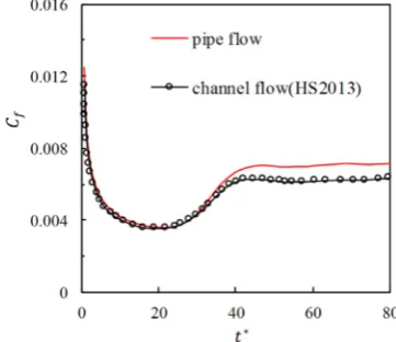
U02) which also reflects the develop-ment of wall shear stress.Fig. 2shows the development ofCfof thepresent pipe flow together with that of a channel flow for compari-son. Prior to the commencement of the acceleration, the friction co-efficient is equal to the value (Cf0=0.00928) corresponding to the initial steady-state flow atRe0=2650.
Immediately after the commencement of the acceleration, it in-creases rapidly to a much higher value, reaching a maximum at (t∗=0.22 when the acceleration is terminated. The value then
re-Fig. 2. Development of friction coefficient.
duces gradually, reaching a minimum value at aroundt∗= ∼21 or t+0=92 (the corresponding time for the channel flow ist∗=21 or
t+0=90). Subsequently,C
frecovers and approaches the steady flow
value of the final flow aroundt∗=42. Then, it only changes slightly untilt∗= ∼50, and remains constant afterwards. It is seen that the trend of the development of the friction factor is the same as that of the transient channel flow of HS2013. In fact, the friction factors of the two flows are practically the same beforet∗=30. In addition, the time for the transition onset is the same in the two flows. Simi-lar to the channel flow, the response can be characterized into three stages; namely pre-transition (t∗<21), transition (t∗=21–42) and fully developed stage (t∗>42).
[image:3.595.335.516.358.514.2]Fig. 3.Transient boundary layer behaviour of pipe flow and channel flow.
These are based on the perturbation velocity ¯u∧defined in a way similar to that used in HS2013, but it is modified for the cylindrical coordinate.
¯
u∧
(
r,t∗)
=u¯(
r,t∗)
−u¯(
r,0)
uc(
t∗)
−uc(
0)
(5)
R2−
R−δ
∗du
2=
R
0
(
1−u¯∧
(
r,t∗))
2r dr (6)R2−
(
R−θ
du
)
2=R
0
¯
u∧
(
r,t∗)(
1−u¯∧(
r,t∗))
2r dr (7)Reθ=
θ
duuc(
t∗)
ν
(8)H=
δ
du∗θ
du(9) where, ¯uanducare ensemble-averaged local streamwise mean
ve-locity and the centre veve-locity of the pipe flow, respectively.
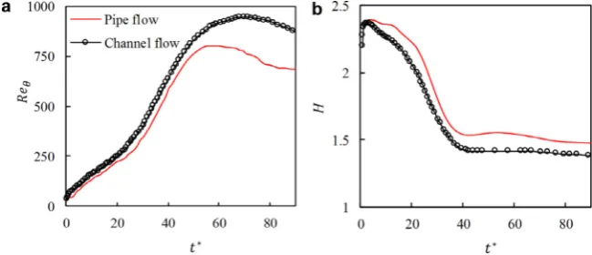
Overall, the boundary layer in a pipe develops in a way similar to that of the channel flow.Reθgrows almost linearly with time until Reθ≈240. Afterwards, the growth rate increases as a result of the on-set of the transition. The value ofReθof the pipe flow is close to, but lower than that of the channel flow during the pre-transition and the transition periods, and diverges from it after the transition is com-pleted (t∗>42). That is, even though the values ofReθ are signifi-cantly different in the two flows they are very close during the tran-sition period. The shape factor of the pipe flow shows a similar devel-oping pattern to that of the channel flow but with a higher value. 3.2. Instantaneous flow
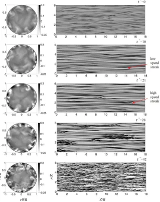
Fig. 4shows the contours of the streamwise fluctuating velocity uzat ar–
θ
plane (z/R=5.0) and az–θ
plane (y+0=5.4, wherey+0is the radial distance from the wall normalized with
ν
/uτ0) at sev-eral instants following the rapid increase of flow rate. The first frame (t∗=0) corresponds to the steady flow field just before the start of the transient flow. It is seen from thez–θ
plane that the values of uzare relatively low and the colour is light. Some weak and shortpatches of high-speed (dark color) and low-speed (brighter color) patterns are present in the initial flow field. Ther–
θ
plane shows that these streaks appear alternately in the azimuthal direction and the low speed streaks penetrate deeper into the core region of the pipe (Klebanoff et al., 1962). Duringt∗=0–21, elongated streaks of posi-tive and negaposi-tiveuz’are formed and intensified. Ther–θ
plane plotson the left show that the low- and high-speed streaks are confined to the region very close to the wall. Later, some highly fluctuating veloc-ities are seen to form, which appear as isolated turbulent patches (or, spots, see panel att∗=28). The spots spread into the flow and merge with each other until aboutt∗=42, when the turbulence occupy the z–
θ
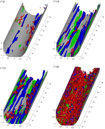
near plane.To further illustrate the flow structures, Fig. 5shows the iso-surface plots ofuz/Ub1and
λ
2att∗=0, 14, 21, and 42. Only the bot-tom half of the pipe is displayed.λ
2is the second eigenvalue of the symmetric tensorS2+2whereSand
are the symmetric and an-tisymmetric parts of the velocity gradient tensor
∇
u. This value is introduced byJeong and Hussain (1995)to identify vortex cores, and has been used frequently in studies of transition and turbulence. At t∗=0, there are few short low- and high-speed streaks. At a later pre-transition stage (t∗=14), elongated streaks appear alternately, which start to break up att∗=21 at some isolated places in the pipe. Packets of hairpin-like structures (identified by the iso-surface of the negativeλ
2) are observed mostly surrounding the low-speed streaks. There are very few of such structures in the early pre-transition stage, and the size of such packet is small; but att∗=21, large spots of the turbulence start to occur, which signify the onset of transition. At the end of the transition (t∗=42), fine vortical structures are full of the flow. The development of the streaky and vortical structures during the transient flow exhibits a great resemblance to that of the channel flow of HS2013.The streamwise and spanwise correlation coefficients of the streamwise velocity, R11, contain quantitative information of the streaky structures.Fig. 6(a) and (b) shows the profiles ofR11at sev-eral instants. It is seen that the magnitude of the negative value of the spanwise correlation increases slightly first and then remains largely unchanged during the early pre-transitional stage (t∗= 4–17). The minimum values of the pipe flow at onset of transition are -0.21, whereas those for channel and boundary layer flow are 0.3, and -0.35 respectively (HS2013). The distance at which the minimum R11 occurs decreases from the highest value∼0.3R (∼50uv
τ0) rapidly to a
minimum∼0.23R (∼70uv
τ, or∼41uvτ0) at pre-transition stage and it
reduces to a value∼0.12R (∼50uv
τ, or∼122uvτ0) at final steady stage.
The averaged spanwise spacing of the streaks at the onset of tran-sition is therefore approximately 0.46R (∼140uv
τ0), which is about
twice the boundary thickness (based on ¯u/u¯c) and is different from
the typical steady flow value of 0.6R (∼100uvτ). The growth of the streaks in streamwise can be observed fromFig. 6(b). The length of the streaks grows from∼3.5R (or∼630uv
τ0) to∼4.5R (or∼1350
v
uτ)
att∗= 21, showing the elongation of the streaks during the pre-transition period. It reduces to∼2.4R (or∼1000uvτ) at the final stage (t∗=97), commensurate with the characteristics of a steady turbu-lent flow at a higher Reynolds number.
3.3. Flow statistics
3.3.1. Mean velocity
[image:4.595.42.291.266.386.2]Fig. 4.Development of flow structure (2-D). Left: Contour plots of (uz/Ub1) in ar–θplane (z/R=5.0); right: contour plots of (uz/Ub1) in az–θplane (y+0=5.4). bright: low speed streaks; dark: high speed streaks.
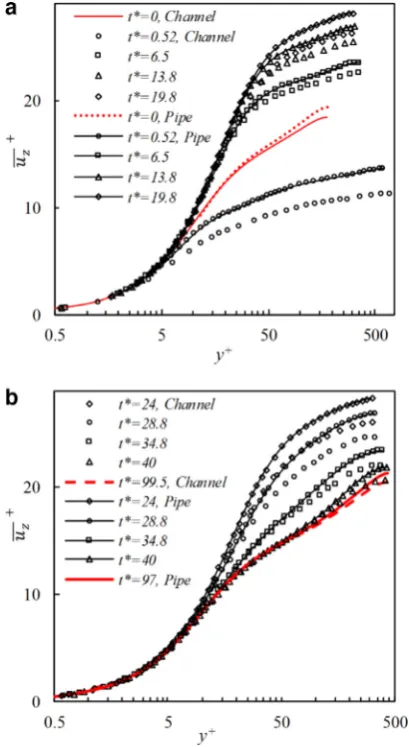
pre-transitional period, after a rapid reduction at the very begin-ning, the velocity gradually increases with time reaching a maximum around the onset of the transition. During this period, the thickness of the sub-layer increases due to the growth of the boundary layer. During the transition period, the velocity in the core progressively reduces and the profile gradually approaches the typical distribution of a steady flow again. It can be seen that the behaviour of the veloc-ity profiles in the pre-transition stage (Fig. 7(a)) is very similar to that in the channel flow. There are however some quantitative differences between two flows. At the initial steady flow, the velocity profiles in the pipe and channel flows overlap each other iny+≤20, but differ beyond this region.
During the pre-transition period, the profiles in the two flows are very similar. In a steady pipe flow, the velocity in the centre region is higher than that in the channel flow. The quantitative differences in the centre region still remain during the pre-transition period. This is due to the fact that both flows respond to the increase of the flow rate as a “plug” flow due to the ‘inertia effect’, namely, the velocity of the fluid is uniform across any cross-section of the pipe perpendicular to the axis of the pipe, and reduces rapidly to zero in the vicinity of the wall due to no-slip boundary condition on the wall. The turbulence in centre region is frozen so that the mean velocity profile does not change. During the transition period, the profiles of both the pipe and the channel flows reduce significantly in the log law region during
t∗=28.8–34.8. The quantitative differences reduce towards the later stage of the transition and at the end, the main differences between the two profiles are in the wake region.
3.3.2. Development of Reynolds stresses
Fig. 8 shows the development of the ensemble-averagedr.m.s. value of the fluctuating velocities normalized by the final bulk ve-locity (uz,rms/Ub1,ur,rms/Ub1, uθ,rms/Ub1), together with the normal-ized Reynolds stress (uzur/Ub12). The curves with makers are data of channel flow at corresponding positions. The responses in the wall region (y+0<36) are shown inFig. 8(a), (c) and (e) and those in the core region are shown inFig. 8(b), (d) and (f). It is clear that the re-sponse of turbulence is different in the wall and in the core regions. In addition, the response of the streamwise turbulenceuz,rmsis char-acteristically different from those of the other two components. Fo-cusing on the streamwise turbulence first, the values ofuz,rmsin the wall region (y+0= 8.6, 19.5) increase rapidly with small or no de-lays untilt∗<34, after which they reduce and eventually approach the steady state values. The response ofuz,rmsat other locations all
have some delays before increasing, the length of which increases with the distance from the wall. In the wall and buffer regions,uz,rms over-shoots its final steady values att∗= ∼30. The responses ofur,rms
Fig. 5. Development of the streaks and vortex structures at several instants: 3-D iso-surfaces plots of low- and high-speed streaks (blue foruz/Ub1= −0.13 and green foruz/Ub1= 0.13);λ2(red forλ2= −2, normalized by (up0/R)2). (For interpretation of the references to colour in this figure legend, the reader is referred to the web version of this article.)
Fig. 6. Profiles of spanwise (a) and streamwise (b) correlations of the streamwise velocity aty+0=5.4.
reduce then increase slightly or remain more or less unchanged until t∗= ∼21.
They then respond rapidly and reach to their corresponding final steady values (or slightly over-shooting them) just aftert∗= ∼35. In the core region, the response ofur,rmsanduθ,rmsare similar to that ofuz,rms, which show a delay followed by a period of response and
the period of the delay is longer as the distance to wall increases. The Reynolds stress inFig. 8(g) and (h) exhibits similar features described for the normal stresses.
[image:6.595.141.467.508.647.2]Fig. 7.Development of ensemble-averaged streamwise mean velocity: (a) pre-transition stage (b) pre-transitional and fully developed stage.
their measurements were largely limited to the core and the buffer region (up toy+0∼ 17). The turbulence behaviour was explained by relating them to turbulence production, energy redistribution be-tween its components and the radial diffusion. The results inFig. 8 provide detailed information in the wall region (y+0<36). More im-portantly, the present results show that the initial response inuz,rmsis due to the formation of elongated streaks which are not conventional turbulence. The rapid increase ofur,rmsanduθ,rmsat aroundt∗= ∼21
is linked to the transition of the flow, from an agitated laminar flow to a turbulent flow. This is to some extend related to the energy re-distribution identified byHe and Jackson (2000).
Comparing the pipe flow with the channel flow, the overall be-haviour identified here is very similar. Especially, in the near wall re-gion, the transient behaviour ofuz,rmsis quantitatively similar before t∗<25. However, some notable differences are observed in the cen-tre region. Firstly,uz,rms,ur,rms,uθ,rms aty+0= 148 increase earlier
in pipe flow than in the channel flow. Secondly, the growth rates of ur,rmsanduθ,rmsare similar before the onset of transition, however
they become larger after the onset of transition in the pipe flow. One possible reason for these differences is that the structures are free to grow in spanwise in the channel flow, whereas in the pipe flow, the structures near the core region are constrained in the azimuthal di-rection. Stronger structure interactions in the pipe core region hence intensify the mixing of the flow, introducing an earlier growth of fluc-tuation velocities and a higher growth rate.
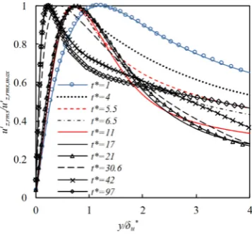
The growth rate of the peakr.m.s.of the fluctuating velocity rep-resents the energy growth in the pre-transition stage.Fig. 9shows the development of the streamwise fluctuating velocity normalised by its corresponding peak value in pipe flow, againsty/
δ
u∗, whereδ
u∗is defined as follows:
¯
u
(
r,t∗)
=u(
r,t∗)
uc(
t∗)
(10)
R2−
(
R−δ
∗u
)
2
=
R
0
(
1− u¯
(
r,t∗))
2rdr (11)The position of the peak value moves rapidly outwards at the be-ginning, then remains almost unchanged at 0.75
δ
u∗duringt∗=5–21. It is of interest noting that the location of the peak value of the transient pipe flow is similar to that found for the channel flow, which remains unchanged duringt∗=5–21 at 0.75
δ
u∗. As indicatedby HS2013, this behaviour suggests thatuz,rmsvalue varies with the
growth of the boundary layer and can be scaled with boundary thick-ness instead of the inner scaling. This is in fact an important feature of the boundary bypass transition reported (e.g.Cossu et al., 2009).
Fig. 10(a) and (b) shows the growth of square of the peakr.m.s. of fluctuating velocities together with the turbulent kinetic energy for both the pipe and channel flows. It is clear that following a short delay, the peak value grows linearly during pre-transition. It is esti-mated that at the onset of transition, the streak amplitude (uz,rms) grows to∼14% of mean flow, which is the same as that of the channel flow (HS2013). The growth rates of the pipe and channel flows are the same beforet∗<21. However, after that, and the growth rates of all components are different in the two flows.
[image:7.595.55.260.56.430.2]3.3.3. Turbulent viscosity
Fig. 11shows the development of turbulent viscosity (
μ
t)calcu-lated from
μ
t=ρ
uzur
duz/dy
(12) The turbulent viscosity reflects turbulent activities and mix-ing, and useful parameter in RANS modelling. It can be seen from Fig. 11(a) that duringt∗=0–19.5, the value of
μ
t/μ
in the corere-gion (y+0>60) remains more or less unchanged (except for some fluctuations) but it decreases in the wall region (y+0<60). During the transition period (21<t∗<42),
μ
t/μ
increases rapidly near thewall (y+0<60), reaching its final steady values towards the end of this period (seeFig. 11(b)). The increase of
μ
t/μ
in the core regionis much slower, which continues after the completion of transition (t∗=43). The behaviour of
μ
t/μ
in the channel is generally the samewith that of the pipe flow. The steady state value is slightly lower in the pipe flow than in the channel flow, especially in the centre region (y+0>50). It is interesting to see that this difference in the centre re-gion (y+0>50) is reduced during the transition stage (21<t∗<43),
but it is regained when the flow is fully developed again. As indicated inSection 3.3.2, the growth of turbulent shear stress (uzur) in the
cen-tre region is different for the two types of flows during the transition stage. The value ofuzurgrows faster in the pipe flow at this stage. However, this is not reflected in the turbulence viscosity response, which implies different growth behaviours of velocity gradient in the two flows. This is discussed in the next section.
3.3.4. Vorticity Reynolds number
Gorji et al. (2014)showed that the
γ
−Reθtransitional model can predict the basic features of a ramp-up flow rather well. However, the predicted onset of the transition in three ramp-up flow cases by this model is noticeably delayed. A key feature of this turbulence model is to make use of the correlation betweenReθandRev.max, replacingFig. 8. Development of the normalizedReynolds stresses. (a, c, e, g) near-wall region; (b, d, f, h) core region. Lines: pipe flow, lines with makers: channel flow.
be evaluated in this section. The vorticity Reynolds numberRevwas originally defined by vanDriest and Blumer (1963). It reads
Reν=
ρ
μ
y2 duzdy (13)
where uz is the local mean velocity. It is known that (Driest and Blumer, 1963; Langtry, 2006) the maximum value of this local pa-rameter (Rev.max) can be directly linked to the momentum thickness
Reynolds numberReθthrough an empirical correlation. HenceRev.max
is used in favour ofReθto avoid the integration of the boundary layer velocity profile in order to determine the onset of transition in the RANS approaches. In the Blasius boundary layer, the maximumRev in the wall-normal direction is proportional to the momentum thick-ness Reynolds number asRev.max=2.193Reθ. For a flat plate boundary
Fig. 9. Development ofurmsnormalized by the peak value.
Fig. 12(a) and (b) shows the developments of the vorticity Reynolds number (Rev) in the channel and pipe flows. The calcula-tion ofRevis based on local mean velocity. It is shown inFig. 12(a) that this local parameter increases quickly near the wall (y/R<0.4), forming a local peak. Another peak is observed at the centre, how-ever, it does not respond to the flow rate change. This is consistent with earlier observations that there are no structural changes in cen-tre region.Fig. 12(b) shows thatRevin the centre (y/R>0.4) increases quickly during the transition stage, whereasRevnear the wall starts to decrease. InFig. 12(c), the development of peakRevagainst theReθ in pipe flow is shown, whereReθ is calculated from the local mean velocity. It is found that the relationship betweenRev.maxandReθis
not linear. The values ofReθandRev.maxat the onset of transition are
395 and 281, respectively.
Let us now consider the differential velocity ( ¯u∧defined inSection 3.1). The correlations between Rev.max
(
u¯∧)
andReθ(
u¯∧)
, which arecalculated from the differential velocity are calculated for both the pipe and channel flows.Fig. 12(d) shows that the near wall peaks, Rev.maxof the pipe and channel flows both increase linearly with the Reθ fort∗<14. After that,Rev.maxin the pipe flow increases slightly
slower thanReθ untilt∗=19.8. In the transitional stage,Rev.max
in-creases significantly slower thanReθ. It shows that there is a linear relationship betweenReθ andRev.maxat the pre-transition stage if
these parameters are calculated from the differential mean velocity. The linear correlation between theRev.maxandReθ in the transient
pipe and channel flows are respectively as:
Reν,max=0.99Reθ (14)
Reν,max=0.62Reθ (15)
The differences between the actual momentum thickness Reynolds number and the prediction of equations are less than 22%
Fig. 11. Development of turbulent viscosity: (a) pre-transition stage (b) transition and fully turbulent stages.
and 14% respectively for the two equations during the pre-transition region (t∗=0–19.8). As shown inSection 3.1, the growth ofReθis the same in the channel and pipe flows during pre-transition. The differ-ence between theRev.max–Reθcorrelation in the two flows is
there-fore attributed to the different growth rates of the vorticity Reynolds number, which are in turn due to the different growths of the ve-locity gradient in these flows. Initially (t∗=0–14), the growth of the velocity gradient of the pipe flow is faster than that of channel flow, but later (t∗=14–19.8), the growth of velocity gradient of pipe flow slows down dramatically, contrasting to the steady growth of the ve-locity gradient in channel flow.
Consequently, the Rev.max–Reθ correlation is geometry
[image:9.595.69.248.56.222.2]depen-dent. This may have some implications when the models devel-oped based on the boundary layer correlation are directly used for a
[image:9.595.133.458.591.727.2]Fig. 12. Development of vorticity Reynolds number (Rev). (a) Pre-transition; (b) transition and fully turbulent stages; (c) relationship betweenReν,maxandReθat pre-transition stage (based on local mean velocity); (d) relationship betweenReν,maxandReθat pre-transition stage (based on differential mean velocity). Lines with makers: pipe flow; makers: channel flow.
channel, pipe or other internal flows. Further studies are required to develop a better understanding.
3.3.5. Budget terms
In this section, we present the variations of the budget terms of uzuzduring the transition period. The transport equation ofuzuzin a
cylindrical coordinate system is as follows:
∂
uz2
∂
t = −2uruz∂
uz∂
r +2p∂
uz∂
z −2∂
puz∂
z− 2 Re
∂
uz∂
z 2+
∂
uz∂
r 2+ 1 r2
∂
uz∂θ
2−1 r
∂
ruruz2∂
r +1
Re
1
r
∂
∂
r ruz2
∂
r(16)
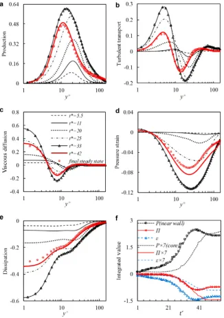
[image:10.595.41.296.490.585.2]On the right hand side of the equation, the terms from left to right are production, pressure strain, pressure diffusion, dissipation rate, turbulent transport and viscous diffusion, respectively. The pressure diffusion term is 0, which is not studied in the following section.
Fig. 13shows the budget terms ofuzuznormalized withuτ4R/
ν
at t∗=5.6, 11, 20, 25, 33, 42. The budget terms of the final steady flow (t∗=97) are shown for comparison. Since the data is normalized us-ing the ensemble-averaged friction velocity (uτ) at the corresponding t∗, the absolute variations during the transitional period cannot be shown. Instead, they show how the distributions deviate from those of a fully developed flow. At the beginning of the transient (t∗=5.6), the budget terms are very low compared to the final flow results. This is due to the rapid increase of the wall shear stress.There are characteristic differences between the budget distribu-tions in the transient flow and in a steady turbulent wall shear flow.
Firstly, the location of the peak production moves fromy+=10 in steady flow toy+=20. Secondly, the dissipation term remains rather uniform in the wall region (say,y+<20), whereas a typical feature of the wall shear flow is that the dissipation increases as the wall is ap-proached. Thirdly, as noted before, the pressure–strain term remains very low compared to the production term, which implies that lit-tle energy is supplied toururanduθuθ. These features of the budget
terms are related to the fact that the “turbulence” generated during the pre-transition stage is not conventional turbulence, but due to the elongated streaky structures (t∗<20).
Fig. 13(f) shows the response of the production (P), pressure strain (II) and dissipation (ɛ) terms integrated over y+0 ≈ 0–50 andy+0≈50–100 respectively. All three terms are normalized with Ruτ04/
ν
to show the absolute value of the development of these terms in the two regions. During the pre-transition period (t∗<21), the pressure strain term remains unchanged in both regions. The pro-duction and dissipation terms grow steadily in the near wall region, but no significant changes are observed in central region. The produc-tion term is mainly balanced by the dissipaproduc-tion term at pre-transiproduc-tion stage in the near wall region, whereas it is balanced by both the pres-sure strain term and dissipation term in the central region. The values of the three terms in centre region are multiplied by 7 for clearer dis-play. Therefore, the production and dissipation terms in the near wall region are much larger than those in the centre region for the flow studied herein.The growths of the budget terms in the near wall region dur-ing the early period (t∗<20) are not associated with conventional turbulence, but a reflection of the streaks developed in the region ofy+0≈0–50. Later during the transition period (t∗=21–40), the
Fig. 13.Development of budget terms ofuzuz: (a) production; (b) turbulence transport; (c) visocus diffusion; (d) pressure strain; (e) disssipation; (f) Spatial integration of (a, d, e)
in the wall and core regions.
significantly. The dominant terms are still production and dissipation in the region ofy+0 ∼ 0–50. However, the pressure strain term in-creases to a significant level in both the near wall and the central re-gions. It starts to overtake the dissipation fort∗>40 in the region ofy+0 ∼ 50–100, where it redistributes a significant amount of en-ergy from the streamwise component to the other two components. The budget terms reach a peak att∗≈40, and then they drop to the steady state values att∗≈44.
3.3.6. Effect of starting and final Reynolds numbers
The results discussed so far have been for a fixed starting and fi-nal Reynolds number. An interesting question to ask is that what will happen if the starting or the final Reynolds numbers are changed. Potentially, the transient process may be affected by a number of factors, including the initial turbulence characteristics (dependent onRe0), the ‘free stream’ velocity (dependent onRe1), the change rate of the mean velocity (dependent on
(
Ub1−Ub0)
/t), and the free stream turbulence level (dependent onRe0andRe1). The rate of
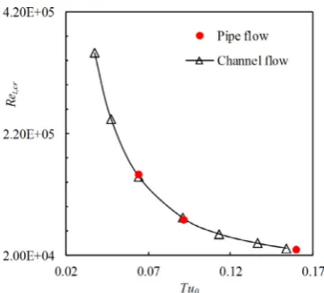
change of the mean velocity plays a weak role as long as the accelera-tion time is much less than the onset time of the transiaccelera-tion (HS2013). It was shown that, in a channel flow, the critical Reynolds number Ret,cr (=tcr∗Re1) is proportional toT u0−1.71, wheretcr∗is the time
for the onset of transition,T u0is defined as
(
urms0,max)
/Ub1,urms0,maxis the peak value of ther.m.s.of the streamwise fluctuating velocity of the initial flow. InFig. 14, the results of three cases of pipe flows with the same initial Reynolds number (Re0=2650) but different fi-nal Reynolds numbers (Re1=3000, 5220, 7362) are plotted against the data obtained from channel flows (He and Seddighi, 2015). Those cases are simulated with the same mesh setup described inSection 2 for the case (Re=2650–7362).
Fig. 14. Transition onset Reynolds number againstT u0.
4. Conclusions
It has been shown that, similar to that in a channel, the tran-sient flow in a pipe after a step increase in flow rate is effectively a laminar flow followed by a bypass transition. New turbulence gen-erated through bypass transition mechanisms initially occupies the near wall region; it propagates into the centre region following the completion of the transition. The general trends of the transition in the pipe and channel flows are found to be the same in the near-wall region. The similarities among the two flows are not only in instan-taneous flow structures, but also in the ensemble-averaged statistical values. However, there are detailed differences in the central region between the two flows during the transition stage. The growth of tur-bulence in the pipe at this stage is faster than that in the channel. This is attributed to the stronger mixing effect in the pipe, where the spanwise space becomes narrower as the flow goes closer to the cen-tre. The developments of the mean velocity profiles, turbulent vis-cosity, vorticity Reynolds number and budget terms are analysed. It is found that the growths of the turbulent viscosity and the vortic-ity Reynolds number are quantitatively different in the two flows, which are attributed to the differences in the velocity gradient velopments. These results may provide useful information for the de-velopment of turbulence models.
Acknowledgements
We gratefully acknowledge that the work reported herein is par-tially funded by UK Engineering and Physical Sciences Research Coun-cil (Grant No. EP/G068925/1). KH is jointly sponsored by Chinese Scholarship Council and The University of Sheffield.
References
Akhavan, R., Kamm, R.D., Shapiro, A.H., 1991. An investigation of transition to turbu-lence in bounded oscillatory Stokes flows. Part 1. Experiments. J. Fluid Mech. 225, 395–422.
Andersson, P., Berggren, M., Henningson, D.S., 1999. Optimal disturbances and bypass transition in boundary layers. Phys. Fluids 11, 134.
Brandt, L., Schlatter, P., Henningson, D.S., 2004. Transition in boundary layers subject to free-stream turbulence. J. Fluid Mech. 517, 167.
Colombo, A.F., Lee, P., Karney, B.W., 2009. A selective literature review of transient-based leak detection methods. J. Hydro-environment Res. 2, 212.
J. Fluid Mech. 514, 65–75.
Gorji, S., Seddighi, M., Ariyaratne, C., Vardy, A.E., Donoghue, T.O., Pokrajac, D., He, S., 2014. A comparative study of turbulence models in a transient channel flow. Com-put. Fluids 89, 111.
He, S., Jackson, J.D., 2000. A study of turbulence under conditions of transient flow in a pipe. J. Fluid Mech. 408, 1.
He, S., Jackson, J.D., 2009. An experimental study of pulsating turbulent flow in a pipe. Eur. J. Mech. B/Fluids 28, 309.
He, S., Ariyaratne, C., Vardy, A.E., 2008. A computational study of wall friction and tur-bulence dynamics in accelerating pipe flows. Comput. Fluids 37, 674.
He, S., Seddighi, M., 2013. Turbulence in transient channel flow. J. Fluid Mech. 715, 60. He, S., Seddighi, M., 2015. Transition of transient channel flow after a change in
Reynolds number. J. Fluid Mech. 764, 395.
Jacobs, R.G., Durbin, P.A., 2001. Simulations of bypass transition. J. Fluid Mech. 428, 185. Jeong, J., Hussain, F., 1995. On the identification of a vortex. J. Fluid Mech. 285, 69. Kataoka, K., Kawabata, T., Miki, K., 1975. The start-up response of pipe flow to a step
change in flow rate. J. Chem. Eng. Japan 8, 266.
Kim, J., Moin, P., 1985. Application of a fractional-step method to incompressible Navier–Stokes equations. J. Comput. Phys. 59, 308.
Klebanoff, P.S., Tidstrom, K.D., Sargent, L.M., 1962. The three-dimensional nature of boundary-layer instability. J. Fluid Mech. 12, 1.
Langtry, R.B., 2006. Correlation-based Transition Modelling for Unstructured Parallelized Computational Fluid Dynamics Codes. University of Stuttgart (Ph.D. thesis).
Maurizio, Q., Stefano, S., 2000. Numerical simulation of turbulent flow in a pipe oscil-lating around its axis. J. Fluids Mech. 424, 217–241.
Maruyama, T., Kuribayashi, T., Mizushina, T., 1976. The structure of the turbulence in transient pipe flows. J. Chem. Eng. Japan 9 (6), 431–439.
Meseguer, A., Trefethen, L.N., 2003. Linearized pipe flow to Reynolds number 107. J. Comput. Phys. 186, 178.
Mizushina, T., Maruyama, T., Hirasawa, H., 1975. Structure of the turbulence in pulsat-ing pipe flow. J. Chem. Eng. Japan. 8 (3), 210–216.
Mankbadi, R.R, Liu, J.T.C., 1992. Near-wall response in turbulent shear flows subjected to imposed unsteadiness. J. Fluid Mech. 238, 55–71.
Nagarajan, S., Lele, S.K., Ferziger, J.H., 2007. Leading edge effect in bypass transition flow. J. Fluid Mech. 572, 471.
Nagib, H.M., Chauhan, K.A., 2008. Variations of von Kármán coefficient in canonical flows. Phys. Fluids 20, 101518.
Ovchinnikov, V., Choudhari, M.M., Piomelli, U., 2008. Numerical simulations of boundary-layer bypass transition due to high-amplitude free-stream turbulence. J. Fluid Mech. 613, 135.
Orlandi, P., 2001. Fluid Flow Phenomena: A Numerical Toolkit, 2001. Kluwer. Seddighi, M., He, S., Vardy, A.E., Orlandi, P., 2014. Direct numerical simulation of an
accelerating channel flow. Flow Turbul. Combust. 92, 473.
Seddighi, M., He, S., Vardy, A.E., Orlandi, P., 2011. A comparative study of turbulence in ramp-up and ramp-down unsteady flows. Flow Turbul. Combust. 86, 439–454. Seddighi, M., 2011. Study of Turbulence and Wall Shear Stress in Unsteady Flow over
Smooth and Rough Wall Surfaces. University of Aberdeen (Ph.D. thesis). Schlatter, P., Brandt, L., de Lange, H.C., Henningson, D.S., 2008. On streak breakdown in
bypass transition. Phys. Fluids 20, 101505.
Wosnik, M., Castillo, L., George, W.K., 2000. A theory for turbulent pipe and channel flows. J. Fluid Mech. 421, 115.
Wu, X.H., Moin, P., 2008. A direct numerical simulation study on the mean velocity characteristics in turbulent pipe flow. J. Fluid Mech. 608, 81.