Novel methods for quantifying movement behavior of free ranging fish from telemetry data

(1)

0

Novel methods for quantifying movement behavior

of free-ranging fish from telemetry data

by

Kilian Michael Stehfest BSc, MRes

This thesis is submitted in partial fulfilment of the requirements for the degree of Doctor of Philosophy in the CSIRO-UTAS PhD Program in Quantitative Marine Science.

Institute for Marine and Antarctic Studies University of Tasmania, Australia

July 2013

(2)

1 Statements and declarations

Declaration of Originality

This thesis contains no material which has been accepted for a degree or diploma by the University or any other institution, except by way of background information and duly

acknowledged in the thesis, and to the best of my knowledge and belief no material previously published or written by another person except where due acknowledgement is made in the text of the thesis, nor does the thesis contain any material that infringes copyright.

Authority of Access

This thesis may be made available for loan and limited copying and communication in accordance with the Copyright Act 1968.

Statement regarding published work contained in thesis

The publisher of the paper comprising Chapter 2 holds the copyright for that content, and access to the material should be sought from the journal. The remaining non published content of the thesis may be made available for loan and limited copying and communication in

accordance with the Copyright Act 1968. Statement of Ethical Conduct

The research associated with this thesis abides by the international and Australian codes on human and animal experimentation, the guidelines by the Australian Government's Office of the Gene Technology Regulator and the rulings of the Safety, Ethics and Institutional Biosafety Committees of the University. All research conducted for this thesis was approved by the University of Tasmania Animal Ethics Committee (Permit No. A0011590).

(3)

2 Statement of Co-Authorship

The following people and institutions contributed to the publication of work undertaken as part of this thesis:

Kilian Stehfest, Fisheries Aquaculture and Coasts, Institute for Marine and Antarctic Studies Dr.Toby Patterson, CSIRO Wealth from Oceans National Research Flagship

Dr. Jayson Semmens, Fisheries Aquaculture and Coasts, Institute for Marine and Antarctic Studies Dr. Laurent Dagorn, Institut de Recherche pour le Développement

Dr. Kim Holland, Hawaiian Institute of Marine Biology (HIMB), University of Hawaii David Itano, Hawaiian Institute of Marine Biology (HIMB), University of Hawaii Dr. Adam Barnett, School of Life and Environmental Sciences, Deakin University

Author details and their roles:

Paper 1, Network analysis of acoustic tracking data reveals the structure and stability of fish aggregations in the ocean

Located in chapter 2

The candidate was the primary author, Toby Patterson and Jayson Semmens are primary supervisors, providing advice on analytical techniques and manuscript preparation. Laurent Dagorn, Kim Holland and David Itano collected the data analysed in this paper. Laurent Dagorn provided advice on manuscript preparation.

Paper 2, Intraspecific differences in movement, dive behavior and vertical habitat preferences of a key marine apex predator

Located in chapter 3

The candidate was the primary author, Toby Patterson and Jayson Semmens are primary supervisors, providing advice on analytical techniques and manuscript preparation. Jayson Semmens assisted with data collection, Adam Barnett collected some of the data analysed and provided advice on manuscript preparation.

We the undersigned agree with the above stated “proportion of work undertaken” for each of the above published (or submitted) peer-reviewed manuscripts contributing to this thesis:

Dr.Jayson Semmens Prof. Colin Buxton

Primary Supervisor Director

Fisheries, Aquaculture and Coasts Fisheries, Aquaculture and Coasts

(4)

3

List of Figures

(7)

6

List of Tables

(8)

7

Abstract

In recent decades, technological progress in the field of biotelemetry has allowed the collection of vast amounts of data on the movement of free-ranging marine animals and recently there have been great advances in analysing data from tags that allow the observation of complete animal tracks. One of the most common and low-cost tools for tracking marine animals, however, are automated acoustic arrays, which often do not record complete tracks but provide presence/absence data for tagged animals at fixed locations. The development of quantitative methods for analysing these data has lagged behind the technological advances in the field.

This thesis applies novel methods for quantifying the movement behaviour of highly mobile free-ranging teleosts and elamsobranchs using automated acoustic tracking data and answers ecological questions of management relevance for tropical tuna (Yellowfin tuna Thunnus albacares) and a temperate shark species (Broadnose sevengill shark Notorynchus cepedianus). Additionally, pop-up satellite archival tag (PSAT) data are analysed for the temperate shark species, to put the findings of the acoustic tracking data analysis into the context of the animals’ large-scale movement behaviour.

(9)

8

locations. For the shark study, receivers were deployed as multiple curtains between opposite shorelines to detect passes of animals through the curtains and determine general movement patterns within a coastal area.

Network analysis methods were applied to both datasets to quantify the co-occurrence of individuals at a given location and to determine the relative importance of each location to the animals. For the former, we adapted association indices from social network analysis to

quantify temporally explicit joint occurrences of individuals. For the latter we treated the number of transitions between locations as a measure of the connectivity between them. The network analysis approach to the acoustic tracking data was well suited to the type of array used in the tuna study and was a considerable improvement over traditional measures of co-occurrence which often only include either the spatial or the temporal dimension, not both. It provided new insight into the temporal dynamics of tuna aggregations at FADs and how they may be linked to between-FAD movement. We observed large interannual variation in

(10)

9

For the shark data, we compared results from the network analysis to a Markovian movement model estimated from counts of observed transitions. Specifically, we tested the suitability of the two methods for determining whether the differences in large-scale movement behaviour between males and females we established from the PSAT data are mirrored in their space-use during their coastal summer residency. Both spatial network analysis and Markov chain analysis showed differences in space-use between male and female broadnose sevengill sharks,

however, rankings of the relative importance of geographic areas differed between the two approaches. This indicated that not only transitions but also residency periods, which are not accounted for by spatial network analysis, were important for identifying priority areas for the sharks.

(11)

10

Acknowledgements

First and foremost, I would like to thank my two supervisors Toby Patterson and Jayson Semmens for their tireless motivation, guidance and support throughout this PhD. It wouldn’t have been possible without them.

I would also like to thank Stewart Frusher and Mark Hindell for their support in the initial stage of my PhD and for making me feel welcome when I first arrived in Tasmania.

I would furthermore like to thank Laurent Dagorn for his collaboration and for making highly productive and enjoyable trips to the Seychelles and Azores possible.

Many thanks go out to Adam Barnett, Laurent Dagorn, Kim Holland and David Itano for letting me play with their data and Jaime McAllister and Russ Bradford for helping me collect my own.

I would also like to extend my gratitude to Bill Holsworth and the Holsworth Wildlife Research Endowment for their generous financial support over the course of my PhD.

(12)

11

Chapter 1 - General Introduction

1.1 Movement ecology: Concepts and significance

Many applied questions in population dynamics and conservation biology have an explicit spatial dimension (Morales et al. 2010). This spatial dimension is fundamentally linked to the movement behavior of individuals (Patterson et al. 2008). As individuals move from one

location to another, they influence not only their own chances of survival and reproduction and the distribution and genetic dispersal of their species (Bowler & Benton 2005), but also the structure and dynamics of the populations, communities and ecosystems they encounter (Nathan et al. 2008). Moreover, movement patterns are likely to play an important role in the response and adaptability of animal populations to perturbations such as overexploitation (Field et al. 2009), disease (Green et al. 2006), habitat loss (Green et al. 2006) or climate change (Drinkwater 2005).

(13)

12

movement ecology paradigm an organism’s movement track is driven by 3 fundamental factors:

1) What is the motivation behind the movement? This question relates to the internal state of an organism and hence the goal of the movement such as finding food or a mate or escaping predation.

2) How is the movement performed? This question relates to the physical capacity of an animal to perform the movement required to reach the goal determined by the internal state.

3) When and to what destination is the movement performed? This question relates to the navigational and sensory capacity of an organism to detect times and/or locations when and/or towards which movement is performed to reach the goal of the movement.

All 3 factors are directly influenced by external environmental factors which can be chemical, physical and biological. Understanding how they interact both with each other and the external environmental factors to produce a movement track and determining the ecological

consequences of the movement track is the overarching aim of movement ecological research (Nathan et al. 2008).

(14)

13

2005), determining the internal state of an individual directly in the field is impossible for most species. Hence, the majority of movement ecological research aims to determine the link between movement patterns and external factors, implicitly acknowledging internal state, movement and navigational capacity without quantifying them.

The main external factors which influence movement tracks can be divided into two categories (Revilla & Wiegand 2008):

(1) Habitats, which includes physical (Morrissey & Gruber 1993) and chemical (Brill 1994) as well as biological parameters such as distribution of prey (Sims et al. 2005)

(2) Interactions with conspecifics, which includes mating (Pratt & Carrier 2001), competition (Jones 1987) and schooling (Newlands et al. 2006).

Habitats in the marine realm exert their influence on movement patterns over a large range of temporal and spatial scales: From transient features such as eddies (Seki et al. 2002) to

(15)

14

Interactions with conspecifics are also likely to exert considerable influence on movement patterns of some species, particularly for animals that inhabit relatively homogeneous habitats and travel in groups such as schooling, pelagic fish (Dagorn et al. 2001). Despite the fact that a large number of commercially exploited fish species fall into this category (e.g. tuna, Partridge et al. 1983, herring, Nøttestad et al. 1996, mackerel, Glass et al. 2006) and that group

movement is likely to influence stock size estimates (Newlands et al. 2006) for these species, only few attempts (Turchin 1989, Turchin 1997) have been made at linking aggregation and movement behavior. This is primarily due to the difficulty of simultaneously collecting movement data on multiple individuals from the same school (Dagorn et al. 2001).

In recent decades, technological progress in the field of biotelemetry (the remote monitoring of an organisms condition, activity, or function, Cooke et al. 2004) has allowed the collection of vast amounts of data on the movement of free-ranging marine animals, providing new insight into the movement ecology of a large range of species. However, the progress of methods for analysing these data has lagged behind in a lot of cases and the potential of biotelemetry for answering the key questions outlined above has yet to be fully exploited.

1.2 Fish tracking techniques: a historical overview

(16)

15

extensive application of this method for a broad range of species started in the 1800s and increased considerably since the 1940s, when the rapid expansion of commercial fisheries after World War II required increased monitoring of exploited fish stocks (Kohler & Turner 2001). Since then, the marking of fish has provided valuable insight into the large-scale movement of a large number of fish species such as cod (Ames 2004), tuna (Eveson et al. 2009) and snapper (Patterson et al. 2001) and is a standard component of the monitoring programs for most commercial fish stocks (e.g. Hallier 2008). However, mark-recapture tagging only provides two locations from the life-history of an individual, the location where it was marked and the location of its recapture, with the latter often highly dependent on the spatial distribution of fishing effort (Sibert & Hampton 2003).

To overcome these limitations, researchers have been working on the development of electronic tags since the 1950s (Arnold & Dewar 2001). These electronic tags can be divided into two broad categories:

(1) data logging tags, which measure and record data on the animal’s environment

(2) transmitter tags, which continuously transmit a signal, making the tagged animal and its location and/or presence detectable to a suitable receiver.

(17)

16

Dewar 2001) and temperature, providing information on the habitat encountered by fish (Metcalfe & Arnold 1997). In the mid 1990s, light level sensors were added to tags deployed on southern bluefin (Gunn et al. 1994) and Pacific bluefin tuna (Itoh et al. 1997), allowing the estimation of geographic position from tag data using geolocation (Wilson et al. 1992) and consequently the reconstruction of the animal’s movement track. Similar to traditional marker tags, however, data loggers relied on the recapture of tagged animals, making them suitable for species with high recapture probabilities i.e. commercially exploited species only. This changed in 1998 when the first pop-up satellite archival tag (PSAT) was developed (Block et al. 1998) and later fitted with a light level sensor for geolocation to study the large-scale movement of

Atlantic bluefin tuna (Block et al. 2001). These PSATs are data loggers which collect and store data, detach from the animal after a predefined period and transmit the collected data via satellite. PSATs are now the standard method for studying the large-scale, open-ocean

movement of non-surfacing marine animals and have provided a wealth of information on the movement ecology of a large variety of species such as turtles (Swimmer et al. 2009), sharks (Bonfil et al. 2005) and marlin (Domeier 2006). Yet, while the development of new statistical methods has considerably improved the reconstruction of animal tracks from geolocation data over the last 10 years (Nielsen et al. 2006, Pedersen et al. 2008, Jonsen et al. 2012), position estimates are still relatively coarse, particularly in coastal areas where sea surface temperature is highly variable and cannot be used to improve geolocation accuracy. Hence, signal

(18)

17

Transmitter tags, which continuously transmit a signal, making the tagged animal and its location or presence detectable to a suitable receiver were first developed for underwater applications by the U.S. Bureau of Commercial Fisheries and the Honeywell Corporation in the 1950s. Tags emitting ultrasonic frequencies (30-300kHz) (Arnold & Dewar 2001), allowing them to be detected by a sonar or hydrophone, were deployed to track the movement of Chinook salmon in the Columbia River (Trefethen 1956). This first generation of tags was relatively large, preventing their use on smaller fish. Additionally, detections of the tag had to be recorded manually (Trefethen 1956), hence only active tracking of single tags was possible and studies using the technology focused on the small-scale movement of individual fish (Voegeli et al. 2001). From the first prototype, tags evolved rapidly and by the early 1960s a smaller tag with twice the detection range and three times the battery-life had been developed (Novotny & Esterberg 1962). In the 1970s, multichannel tags which could measure both internal and

external temperature (Carey & Lawson 1973) or swimming speed (Scariotta & Nelson 1977) and transmit the data through ultrasonic codes were developed, vastly increasing the biological and behavioral information that could be collected. However, receivers were still only capable of active or “focal tracking” (Sims 2009) of single tags until the 1980s (Voegeli et al. 2001) and while providing continuous tracks with relatively high position accuracy, actively tracking highly mobile species for long periods of time is prohibitively expensive and has only been carried out for a small number of individuals from a few species (e.g. the blue shark, Carey et al. 1990, marlin, Block et al. 1992). The introduction of commercially available automated receivers in the 1980s (McKibben et al. 1985) which contained a microprocessor and memory

(19)

18

compare acoustic signals to a list of stored signals and thereby identify and distinguish multiple tags and the memory allowed the storage of detection records, removing the need for manual, real-time recording of detections (Voegeli et al. 2001). This allowed continuous monitoring of the presence of multiple tagged individuals at fixed locations over long time periods, such as the presence of hammerhead sharks at seamounts (Klimley et al. 1988) or tuna (Dagorn et al. 2007) or dolphinfish (Taquet et al. 2007) at fish aggregating devices . Since the development of these first automated receivers, acoustic telemetry technology has become almost ubiquitous in marine movement behavior studies (e.g. Lacroix & McCurdy 1996, Klimley & Holloway 1999, Welch et al. 2006, Dagorn et al. 2007) and the reduction in cost of acoustic receivers has meant that monitoring arrays have continuously increased in size with arrays of up to 400 receivers reported in recent studies (Welch et al. 2011). This increase in array size means that the possibilities for array configuration have become increasingly diverse (see Heupel et al. (2006) for review), giving researchers the flexibility to address a wide range of questions regarding the movement of marine fish from the fine-scale movement of reef fish (Bolden 2001) to the large-scale migration of wide-ranging apex predators (Jorgensen et al. 2010).

1.3 Automated acoustic telemetry: Array designs

(20)

19

(1) Single receivers placed at ecologically significant locations such as refuge areas (Meyer et al. 2000), seamounts (Klimley et al. 1988), fish aggregating devices (FADs) (Dagorn et al. 2007) or oil rigs (Lowe et al. 2009). This is the oldest automated acoustic array type (Klimley et al. 1988) and is highly suited to studying different types of aggregating behavior. It has provided

significant insight into the temporal dynamics of residencies (Ohta et al. 2005) and interactions between individuals (Klimley & Holloway 1999) and species (Klimley & Butler 1988) at a given location and is the most cost and labor effective array type. While it can also be used to determine movement rates between multiple such significant locations (Lowe et al. 2009), compared to the other array design types, this generally produces the most rudimentary data in terms of recording animal movement in space and time.

(2) Regular or irregular grid arrays, which are mainly used to study the space-use of fish in well defined study areas such as reefs (Claisse et al. 2011), marine protected areas (MPAs)(Meyer et al. 2010) or coastal embayments (Heupel et al. 2004). This type of array is used to determine general movement patterns at local (meters) to regional (kilometers) scales. Detection probability depends on receiver density and is a trade-off between the size of the study area and the cost of acoustic receivers. If sufficient receivers are deployed that detection ranges overlap, continuous monitoring of fish movement is possible with a positional accuracy equivalent to the receiver range (Heupel et al. 2006). If receivers are only as far apart as the radius of the detection range, positional accuracy of 1-5m can be achieved through

(21)

20

2011), providing complete movement tracks similar to those from active tracking. Receiver grids can be regular, random or stratified by habitat type, depending on the study objective.

(3) curtains or gates of receivers with overlapping ranges to capture the passage of animals, for example along migratory routes (Honda et al. 2010), in longitudinal coastal areas such as estuaries (Andrews et al. 2010) or in and out of MPAs (Barnett et al. 2011). This type of array is generally used to study large-scale movements (Welch et al. 2002) or in study areas too large to make gridded arrays feasible. If receiver density in a gridded array becomes too low, tags might not be detected by the array. Curtains overcome this problem by focusing receiver effort in crucial areas. While this means that tags might only be detected for a small proportion of an animal’s track, detection probabilities can be close to 100% when the animal passes through the curtain (Heupel et al. 2006). If two closely spaced curtains are deployed, direction of travel can be established from subsequent detections at the two curtains (Lacroix et al. 2005). The choice of array configuration depends both on the study objectives and the resources available and can result in widely different types of data (Heupel et al. 2006). Hence the type of data analyses that will be employed should be considered early in the design process to ensure the most efficient use of resources and successful testing of a given hypothesis.

1.4 Automated acoustic telemetry: Data analysis

The main difference in the types of data that can be collected using automated acoustic arrays is whether the temporal and spatial resolution is sufficient for the data to approximate

(22)

21

records at a series of fixed locations. For the former a number of descriptive movement metrics such as swimming speed, turning angle and tortuosity can be calculated (Sims 2009). More recently, a number of methods such as optimal Levy flight (Sims 2009) or state-space modeling (McClintock et al. 2011, Breed et al. 2012, Jonsen et al. 2012, Langrock et al. 2012) have been developed to determine the animal’s behavioral mode such as foraging or transiting from these movement metrics in order to link behavior to spatial location.

(23)

22

spatial dimension of the data. These analytical approaches include survival analysis of residence times (Klimley & Holloway 1999), time series composition to determine periodicity in detection sequences (Ohta et al. 2005) or circular statistics to determine diel rhythms in detections (Barnett et al. 2012a).

Novel quantitative approaches for the rigorous statistical analysis of data from automated acoustic telemetry arrays that include both the spatial and temporal dimensions are required in order to make the most efficient use of the wealth of data collected using this now ubiquitous technique (Heupel et al. 2006, Sims 2009, Jacoby et al. 2012). These novel methods could either be adapted from terrestrial telemetry applications (Heupel et al. 2006), from different scientific disciplines (Jacoby et al. 2012) or from methods for traditional mark-recapture analysis (Heupel & Simpfendorfer 2002), which shares many of the characteristics and problems of acoustic tracking data.

1.5 Network analysis

(24)

23

what constitutes a node and how the connection between nodes is quantified is completely open, network analysis can be applied to a large variety of systems, from a wide range of fields providing insight into networks such as the internet (Doyle et al. 2005), transportation routes (Guimera et al. 2005), human social networks (Liben-Nowell et al. 2005) or metabolic networks (Jeong et al. 2000).

In the field of animal behavior, network analysis has been applied to two different types of networks: (1) animal social networks and (2) spatial ecological networks.

Social network analysis originated in the social sciences in the 1930s (James et al. 2009) to understand patterns of human interactions. The nodes in social networks generally represent individuals and the edges between them some measure of their association. Network analysis has been applied to determine the social structure of a wide range of animal populations, both terrestrial (African elephants, Wittemeyer et al. 2005, African buffalo, Cross et al. 2004,

(25)

24

behaviour as well as individual or species interactions at a given receiver site, which has thus far only been done descriptively (Klimley & Holloway 1999).

In spatial ecological networks on the other hand, nodes represent locations such as habitat patches (Bunn et al. 2000) or roosting sites (Fortuna et al. 2009) instead of individuals and the edges between them represent some kind of ecological flow or connection. Spatial network analysis was first applied to movement ecology by Urban & Keitt (2001) to determine connectivity of different landscapes through American mink and prothonotary warbler movement. Rather than using movement observations, however, they used dispersal

probability based on simple movement rules to quantify connectivity between landscapes. A similar approach was then applied to actual movement observations for the first time to determine the properties of a network of bat roosting sites and identify priority areas for conservation using radio-telemetry data (Rhodes et al. 2006). Since then, spatial network analysis has only recently been applied to a marine species using acoustic telemetry data (Jacoby et al. 2012) and the full range of quantitative methods network analysis provides for the analysis of acoustic telemetry data has yet to be fully exploited.

1.6 Markov chain analysis

(26)

25

stochastic, as transition probabilities are estimated from empirical state sequences rather than being the result of a set of deterministic rules (Johnson et al. 2004).

What constitutes a state is hereby entirely open and Markov chain analysis has been applied to such diverse phenomena as the probability of daily rainfall (Jimoh & Webster 1996), the rate of transition from preclinical to clinical state of breast cancer (Duffy et al. 1995), vegetation succession in response to climate variability (Stephenson et al. 2006) or to model transition probabilities between behavioral states in state-space models of animal movement tracks (Patterson et al. 2009, Langrock et al. 2012, Xydes et al. 2013). In animal movement analysis, Markov chain analysis has also been used to determine transition probabilities between spatial states, i.e. geographic locations or areas, from continuous animal track data (Johnson et al. 2004, Pedersen et al. 2011)

(27)

26

rarely been used to analyse animal movement patterns from automated telemetry data, even though the data is relatively similar to mark-recapture data, as it consists of repeated

presence/absence records of identifiable individuals rather than actual movement tracks. The only Markov chain analysis of fish movement patterns from such data is a study of juvenile salmon migration in a river, using a radio-telemetry curtain array (Steel et al. 2001). However, since the migratory movement of juvenile salmon is unidirectional, the authors did not model movement between discrete spatial states directly. Instead, they estimated river segment specific probabilities of switching between a moving and a holding state based on travel times between curtains.

Hence, even though Markov chain analysis has been applied to mark-recapture data for decades and is increasingly being used to model movement patterns from telemetry data of complete movement tracks, the full potential of Markov chains for analysing automated acoustic telemetry data has yet to be fully realized.

1.7 Thesis objectives and structure

This thesis aims to develop novel methods for quantifying the movement behaviour of highly mobile free-ranging fish using automated acoustic tracking data and answer ecological

(28)

27

movement behaviour, in light of the detection of sex-specific patterns in large-scale movement through pop-up satellite archival tagging (PSATs, Chapter 3).

All data chapters in this thesis have been prepared as independent, self contained manuscripts for publication. Chapter 2 has already been published in a peer-reviewed journal (Appendix 1) and chapter 3 is currently under peer-review.

The first dataset (Chapter 2) consists of acoustic tracking data from yellowfin tuna (Thunnus albacares) at fish aggregating devices (FADs) around the Hawai’ian island of Oahu and represents the type of array that consists of single receivers placed at ecologically significant locations. Social network analyses are applied to the data to determine the frequency and temporal dynamics of spatially and temporally explicit co-occurrences of individual tuna to elucidate the emergent structure and temporal stability of the tuna aggregations. Spatial network analyses are used to quantify movement rates between FADs and link these to the temporal dynamics of the aggregations.

(29)

28

(30)

29

Chapter 2 - Network analysis of acoustic tracking data reveals the structure and

stability of fish aggregations in the ocean

2.1 Introduction

Aggregations in the distribution of individuals are an almost universal phenomenon in living organisms of all sizes, from bacteria to whales (Parrish & Edelstein-Keshet 1999). They can be considered as part of a continuum of group integration, ranging from highly territorial

organisms with minimal group interaction on one end to social animal groups with strong, long-lasting bonds between individuals (Parrish et al. 2002) such as groups of primates (Flack et al. 2006) or marine mammals (e.g. Baird & Whitehead 2000) on the other. Aggregations where animals display collective coordinated movement without forming stable social bonds such as flocks of birds, insect swarms and fish schools fall somewhere between these two extremes (Parrish et al. 2002).

The behaviour of schooling fish has been the subject of many studies, both empirical (e.g. Ward et al. 2002) and theoretical (see Giardina 2008 for review). Yet, while the last few decades have seen a vast amount of data collected on the movement of free ranging animals that display some degree of collective motion (Cooke et al. 2004), the analytical approaches for quantifying collective movement from these data are relatively limited. With a few exceptions (Minta 1992), the majority of studies either determine temporal synchronicity of movement

(31)

30

overlap which uses spatial locations but ignores the temporal dimension inherent in movement data (e.g. Dillon & Kelly 2008; Schuttler et al. 2012).

Network statistical analysis has emerged as a powerful tool for improving our understanding of animal interactions, particularly in fission/fusion societies, where groups are highly dynamic and frequently split and reform (James et al. 2009). Since it relies on the temporally explicit observation of associations between individuals, to date, it has mostly been applied to

(32)

31

Tropical tuna are amongst a number of pelagic fish species that are known to aggregate around floating objects (Fréon & Dagorn 2000; Castro et al. 2002), forming large, multi-species

aggregations (Schaefer & Fuller 2005). While the biological or evolutionary advantage of the association of tuna with floating objects is not known, several hypotheses have been proposed (Fréon & Dagorn 2000; Castro et al. 2002). One of these is the meeting point hypothesis, which suggests that tuna associate with FADs to increase encounter rates with other individuals (Dagorn & Fréon 1999; Fréon & Dagorn 2000; Soria et al. 2009). If this is the case, floating objects play an important role in tuna aggregation behaviour.

(33)

32

While several studies have monitored the behaviour of individual tuna associated with floating objects (Holland et al. 1990; Cayré 1991; Marsac & Cayré 1998; Itano & Holland 2000; Girard et al. 2004; Ohta & Kakuma 2005; Schaefer & Fuller 2005; Dagorn et al. 2007), none of these studies have attempted to quantify the collective movement of tuna in FAD aggregations beyond the description of synchronous departures from and arrivals at a FAD (Klimley & Holloway 1999; Ohta & Kakuma 2005). In this study we used passive acoustic tracking to observe the presence of tropical tuna in an array of 13 FADs around the Hawai’ian island of Oahu. We analysed these data using network analysis in order to; (1) Identify the spatially and temporally explicit co-occurrences of individual tuna; (2) determine the frequency and

(34)

33 2.2 Materials and methods

2.2.1 Data collection

(35)

34

2000; Schaefer & Fuller 2002; Robert et al. 2012b). A scalpel was used to make a 1–2 cm long incision in the muscle of the abdominal wall 3–5 cm anterior to the anus and 2–3 cm to one side of the ventral midline. To avoid possible damage of organs by the scalpel, final entry into the abdominal cavity was made using a latex gloved finger to rupture the peritoneal lining. A coded Vemco V16 tag (69 kHz, V16-4H-R256, 5–30 s delay, rated battery life 344 days) was then inserted in the peritoneal cavity and the wound closed with two absorbable sutures. Tag weight was approximately 24 grams, which constitutes an average of 0.84 % and a maximum of 3.4 % of the total bodyweight of the tagged fish. In order to make tagged fish noticeable to fishermen and maximize reporting of recaptures, all tagged fish were also marked with an external

Hallprint 11 cm plastic dart tag inserted through the pterygiophores of the second dorsal fin. All fish were measured to the nearest cm prior to release. The total elapsed time that the fish were out of water was between 1 and 2 min, with all fish released within 300 m of the FAD of

capture.

Tuna were tagged in three tagging periods: 46 of the tuna were tagged from August to November 2002 and from January to May 2003 and an additional 40 fish were tagged from January to February 2005. Fish tagged in 2002/2003 ranged from 54 to 86 cm in fork length (FL) whereas fish tagged in 2005 ranged from 23 to 83 cm FL. As a previous study has shown a shift in feeding behaviour when yellowfin tuna in the Hawai’ian FAD array grow larger than

(36)

35

2005 were small (<50 cm FL, mean size=36.3 cm) and 16 of medium size (>50 cm FL, mean size=71.2 cm). Tags used in 2002/2003 acoustically transmitted a unique ID code every 5-30 seconds, whereas those used in 2005 transmitted every 30-90 seconds. Tags had a battery life of 344 days, which means overlap between fish tagged in 2005 and those tagged in previous years (2002 and 2003) was not possible. The dataset of detections at the 13 acoustic receivers was therefore split in two and any subsequent analyses carried out separately for the

2002/2003 and the 2005 datasets. Where appropriate, interannual comparisons were only carried out between the 2003 dataset and the medium sized fish tagged in 2005 to remove the potentially confounding effect of fish size.

2.2.2 Animal ethics

All fishing, tagging and general animal handling procedures were in accordance with established best practices used in numerous other studies on similar sized tuna around the world (Klimley & Holloway 1999; Schaefer & Fuller 2002; Ohta & Kakuma 2005; Dagorn et al. 2007; Schaefer et al. 2007). All personnel and procedures were specifically approved by the University of Hawaii Institutional Animal Care and Use Committee (IACUC). The established best practices are designed to minimize negative impacts on the tuna and direct handling of fish was limited as much as possible. No anaesthetic was used as tuna exhibit complete immobility and

insensitivity to touch or manipulation for several minutes when swiftly removed from water (Brill 2002). Furthermore, the negative effects of using anaesthetics would have been

(37)

36

breathers, they would sink to the bottom and suffocate (Brill 2002). Hence the animals would have to be kept in water tanks on the tagging vessel with a water flow velocity similar to the tuna’s normal swimming speed until full recovery, which is not feasible. The total time a tuna spent out of the water was less than 2 minutes and no adverse impact was observed in this study or has ever been reported in any other studies, based on the observation of post tagging behaviour and long detection periods of the tags (up to 150 days in this study). Any fish

determined unfit for tagging due to excessive bleeding from the mouth or injury to the eyes or gills were euthanized with a blow to the head, as recommended under IACUC procedures. The specific type of fishing employed (trolling and jigging) ensured that numbers of these unfit fish were kept to a minimum. Since aggregations at the FADs around Oahu are solely comprised of tropical tuna no other species were captured or harmed as a result of the tagging operations.

2.2.3 Association calculations

In animal networks analysis, association strength is often defined by the “gambit of the group”, i.e. the frequency with which two individuals are found together in the same group (Cairns & Schwager 1987). To determine the frequency of spatio-temporal co-occurrences of tuna in FAD aggregations, we defined a group as all fish present in the receiver range of a given FAD. A pair of individuals (dyad) was therefore considered associated if their acoustic signals were detected by the same receiver within a given time interval, henceforth referred to as the sampling

(38)

37

Kakuma 2005). To test whether ignoring these short term departures from the FAD

aggregations has an impact on association strength between two individuals and to determine the impact of sampling period duration on the association strength between individuals, association indices were also calculated for 1 hour sampling periods and the results compared using a randomized Mantel’s matrix correlation test (Schnell et al. 1985).

To calculate the association index for each dyad, the simple ratio index (SRI), recommended by Ginsberg & Young (1992) was calculated using the SOCPROG 2.4 (Whitehead 2009) extension for MATLAB (MathWorks 2010). For two individuals a and b, the SRI is computed as follows:

Eqn. 1 SRI=X/(X+Yab+Ya+Yb)

With X = the number of sampling periods in which a and b were detected together

Yab= the number of sampling periods in which aand b were observed at different FADs

Ya=the number of sampling periods in which only a was observed

Yb=the number of sampling periods in which only b was observed

For the SRI to be an unbiased measure of the proportion of time two individuals spend together, the dataset has to meet the following assumptions: recorded associations are symmetric and accurate, the probability of identification is independent of whether an

(39)

38

these assumptions, with the main source of possible violations stemming from acoustic signal collision. If an acoustic receiver receives the signals of two fish simultaneously, it might not record either of them, or the two colliding signals may overlap and be recorded as the signal of another tag, leading to the false detection of a fish which is not within receiver range. As the risk of signal collision increases with the number of tags present within the receiver range (e.g. Topping & Szedlmeyer 2011), tagged fish are conceivably less likely to be reliably detected when associated with other individuals. This problem is addressed and to some degree alleviated by the tag manufacturer, as tags transmit their acoustic signal at a random time, between 30 and 90 s, reducing the risk of signal collision. Moreover, the potential of signal collisions to bias the association index can be reduced by using a sampling period that is

relatively large (24 hours) compared to the temporal resolution of the data (10s of seconds) and by removing any potential false detections caused by signal collision. This was accomplished by removing all single records which had no additional detections within 1 hour before or after from the raw dataset.

Another potential source of violating the aforementioned assumptions is the variable range of the receivers, which means that the spatial definition of the FAD aggregation changes, hence a tagged individual just outside the receiver range will not be detected despite being part of the aggregation. However, if this bias exists, it is probably small and approximately constant.

(40)

39

analyses in SOCPROG (Whitehead 2009) and the drawing of sociograms in NetDraw (Borgatti 2002).

2.2.4 Network analysis

To visualize the tuna networks for both 2002/2003 and 2005, the datasets were plotted as sociograms, consisting of nodes and edges, where each node represents an individual and the edge between them an associative link, with the thickness of the lines representing the edges proportional to the given association index.

To test whether the network exhibited preferred associations between individuals rather than being random, we determined if there was a significant difference between real association patterns and those obtained from a large number of random permutations, which were computed as described in Whitehead (2008). As tuna were rarely detected at two different FADs within the same sampling period, the permutation of associations between rather than within sampling periods was chosen, with a null hypothesis of ‘no preferred companionship between sampling periods’. This means that group membership in each sampling period was permuted with the constraint that the number of associations for each animal in each sampling period was kept constant (Whitehead 2009). The coefficient of variation (CV) of the SRI

(41)

40

To determine the structure of the network, the individual mean and maximum of the SRI were averaged over all individuals as well as by individual tagging cohorts (fish tagged at the same FAD on the same day). To test whether associations were higher within cohorts than overall, a randomized Mantel’s matrix correlation test (Schnell et al. 1985) between the association matrix and a binary matrix of whether the individuals of each dyad were from the same (1) or different (0) cohorts was carried out.

2.2.5 Analysis of movement patterns

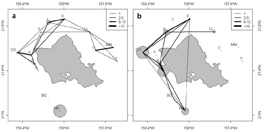
To compare movement patterns of tagged tuna between the two tagging periods and link them to differences in spatio-temporal co-occurrences, directed between-FAD movement rates were summed for all individuals and mapped for the two study periods. Select network metrics were then calculated for the resulting movement networks, where nodes represent the FADs and ties between them represent movement rates (see Jacoby et al. 2012). The chosen network metrics were:

1. Average degree, which indicates the average number of FADs connected to each FAD through direct fish movement.

2. Density, which represents the proportion of direct connections present out of the total number of direct connections possible.

(42)

41

4. Mean strength, which is the mean number of direct movements made to or from each FAD.

2.2.6 Temporal analysis

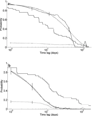
To characterize the temporal dynamics of associations between individuals, the lagged

(43)

42

(MathWorks 2010). The probability of still being detectable and present in the FAD array was then plotted against time lag and compared to the LAR. The assumption is hereby that a decay in the LAR which is more rapid than the associated decay in the survival of an individual in the FAD array, is indicative of actual declines in association, rather than being a result of mortality, emigration or tag failure.

(44)

[image:44.612.82.548.158.531.2]

43

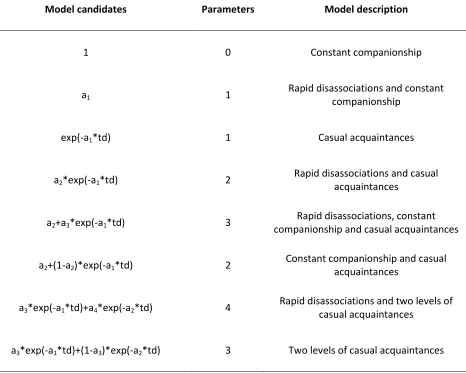
Table 2.1 Negative exponential models of association decay over time fitted to the dataset. a1 -a4 are model parameters, td is the time lag. Models are made up of one or a combination of decay terms describing constant companionship, casual acquaintances and rapid

disassociations (see Model description) (Whitehead 2009).

Model candidates Parameters Model description

1 0 Constant companionship

a1 1 Rapid disassociations and constant

companionship

exp(-a1*td) 1 Casual acquaintances

a2*exp(-a1*td) 2

Rapid disassociations and casual acquaintances

a2+a3*exp(-a1*td) 3 Rapid disassociations, constant

companionship and casual acquaintances

a2+(1-a2)*exp(-a1*td) 2 Constant companionship and casual

acquaintances

a3*exp(-a1*td)+a4*exp(-a2*td) 4 Rapid disassociations and two levels of

casual acquaintances

(45)

[image:45.612.198.419.88.335.2]

44

(46)

45 2.3 Results

2.3.1 Dataset overview

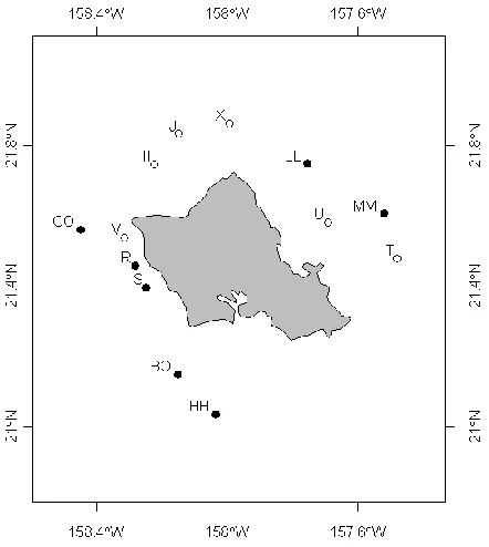
A total of 46 tuna were tagged in the FAD array in 2002/2003 at 5 different FADs (Table 2.2). In 2005, 40 fish were tagged at 5 different FADs, 3 of the tagging FADs were the same as during the 2002/2003 tagging (CO, HH and S). Mean tagging cohort size was similar for the 2 datasets, however, the standard deviation was greater in 2005 (Table 2.2) and the largest cohort was tagged that year (11 YFT tagged at FAD R in January 2005). The mean number of days with detections per individual was similar between 2002/2003 and 2005 whereas the total number of days with detections (i.e. total number of sampling periods) was greater in 2002/2003 due to the fact that tagging occurred over a longer time period. Mean number of fish detected per sampling period was also greater for the 2002/2003 dataset, reflecting the greater number of fish tagged.

(47)

46

2.3.2 Network structure

Associations between individuals were not random, as the coefficient of variation was significantly higher than in the randomized dataset for fish tagged in 2002/2003 (CV=3.69, random CV=3.68, p<0.025), and small (CV=3.26, random CV =3.17, p<0.025) and medium sized fish (CV=1.58, random CV=1.24, p<0.025) tagged in 2005. This indicates that fish associated preferentially with particular individuals over several sampling periods in all cases.

Mean association was highest for medium sized fish in 2005 (>50 cm FL), whereas small fish (<50 cm FL) tagged in the same year had a much lower mean association index. Fish tagged in 2003 (>50 cm FL) had the lowest mean association due to the tagging being carried out over a much longer time period, leading to a large proportion of zero associations (Table 2.3). When comparing the means of non-zero elements, however, fish tagged in 2003 had the highest mean association (SRI=0.321), followed by medium sized fish tagged in 2005 (SRI=0.273), while small fish tagged in 2005 had the lowest mean association (SRI=0.221).

(48)

47

2.3.3 Movement patterns

The 2002/2003 data indicates that individuals were much less likely to associate with individuals tagged at other FADs than in 2005 (Fig. 2.2), when the majority of fish formed associations with fish tagged at other FADs. This is due to the different probabilities to

encounter fish tagged at other FADs between the two years, as more individuals moved to FADs other than their FAD of tagging in 2005 (58 % of all small and 44 % of all medium sized fish) than in 2002/2003 (17 % of all tagged fish). Yet, even though less individuals moved to different FADs, more FADs were visited by tagged fish in 2002/2003 than in 2005 (Fig. 2.3) leading to the greater mean degree and density and lower fragmentation of the movement network in

2002/2003 (Table 2.4). Between-FAD movement rates, however, were greater in 2005 than in 2002/2003 (Fig. 2.3) resulting in a greater mean strength of the movement network (Table 2.4). The large standard deviation of mean strength in 2005 was caused by the large number of movements (21) between adjacent FADs R and S. The greater between-FAD movement in 2005 also meant that detections were spread more evenly across receivers (Fig. 2.3) whereas in 2002/2003 almost half of all detections occurred at a single FAD, which had no connection to any other FADs through direct tuna movement (FAD HH).

(49)

48

highest mean number of associates despite the fact that the largest number of fish was tagged at FAD S (Table 2.3) and there was no significant relationship between mean number of

associates and number of fish tagged (linear model, R2=0.72, p=0.07). Instead, the fish with the largest number of associates in 2005 was an individual that performed multiple between-FAD movements, visiting a total of 5 of the 13 FADs.

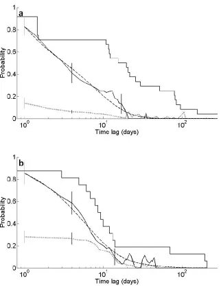
2.3.4 Temporal dynamics

Decay of association between dyads differed considerably between the 2002/2003 and the 2005 dataset. In 2002/2003, the probability to remain associated initially decreased slowly over a time lag of approximately 20 days and only then started to decline steeply (Fig. 2.4a). The LAR crosses the NAR at a lag of approximately 60 days, suggesting that after this lag, association between individuals was random, irrespective of whether or not the dyad was associated previously. In 2005, the LAR steeply declines from the first day and reaches the level of the NAR after a time lag of approximately 20 days (Fig. 2.4b), indicating a much faster decay of

(50)

49

in association might be slower. In 2005 on the other hand the LAR lies below the survival

probability for both size classes, indicating that emigration or removal from the FAD array is not the cause of the steep decay in association.

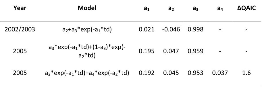
The differences between the 2002/2003 and 2005 data are also evident in the negative exponential models that best fit the two datasets. For 2002/2003, the model of rapid disassociations, constant companionship and casual acquaintances (see Table 2.6 for model parameter values) had the lowest QAIC. For 2005 on the other hand, the model that best fit the data was that of two levels of casual acquaintances (see Table 2.6 for model parameter values), however, there was also substantial support for the model of rapid disassociations and two levels of casual acquaintance (see Table 2.6 for model parameter values). These two model candidates were the best fit for the 2005 data when analysing the two size classes separately as well. Hence, interannual differences in association decay were real and not a result of

(51)

[image:51.612.41.575.128.381.2]

50

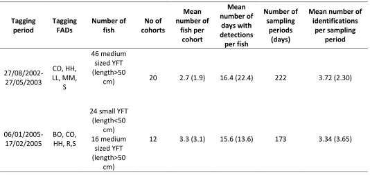
Table 2.2 Dataset overview. For mean values, standard deviation is given in brackets.

Tagging period Tagging FADs Number of fish No of cohorts Mean number of fish per cohort Mean number of days with detections per fish Number of sampling periods (days)

Mean number of identifications per sampling period 27/08/2002-27/05/2003 CO, HH, LL, MM, S 46 medium sized YFT (length>50

cm) 20 2.7 (1.9) 16.4 (22.4) 222 3.72 (2.30)

06/01/2005-17/02/2005

BO, CO, HH, R,S

24 small YFT (length<50 cm) 16 medium sized YFT (length>50 cm)

(52)

[image:52.612.160.455.157.227.2]

51

Table 2.3 Mean SRI for each individual averaged over the dataset as a whole and within tagging cohorts for small and medium sized fish. Standard deviation is given in brackets.

Mean Association 2002/2003 medium 2005 small 2005 medium Within cohorts 0.26 (0.24) 0.30 (0.30) 0.36 (0.24)

[image:52.612.138.475.314.447.2]

Overall 0.04 (0.04) 0.06 (0.07) 0.13 (0.08)

Table 2.4 Network metrics calculated for the tuna movement networks in 2002/2003 and 2005. Movement network

metric 2002/2003 2005

Average degree 2.769 2.154

Density 0.231 0.179

Fragmentation 0.295 0.641

Mean strength 6.31 (4.96) 9.08 (10.54)

Table 2.5 Mean number of associates per individual by tagging FAD and number of fish tagged per FAD. Standard deviation is given in brackets.

FAD Mean number of associates 2002/2003 Number of fish tagged 2002/2003 Mean number of associates 2005 Number of fish tagged 2005

BO - - 4.0 (4.2) 2

CO 7.3 (3.9) 19 5.0 (1.7) 3

HH 4.7 (1.9) 9 8.6 (3.2) 8

LL 1 (-) 1 -

-MM 0 (-) 1 -

-R - - 14.8 (6.8) 11

S 5.3 (3.9) 16 11.7 (4.4) 16

[image:52.612.138.476.549.712.2]

(53)

[image:53.612.79.535.175.329.2]

52

Table 2.6 Negative exponential models and model parameter values of association decay over time which best fit the 2002/2003 and 2005 datasets. Two models and sets of parameter values are given for the 2005 data, as there was substantial support (∆QAIC <2) for a second model (See Table 2.1 for descriptions of models).

Year Model a1 a2 a3 a4 ∆QAIC

2002/2003 a2+a3*exp(-a1*td) 0.021 -0.046 0.998 - -

2005 a3*exp(-a1*td)+(1-a3

)*exp(-a2*td) 0.195 0.047 0.959 - -

(54)

[image:54.612.145.467.75.555.2]

53

Figure 2.2 Sociogram of a) associations between tuna tagged in 2002/2003 and b) associations between tuna tagged in 2005. Ellipses indicate tagging FADs (refer to Fig. 2.1). Nodes represent individual tuna, lines represent edges between them. Line thickness is proportional to

(55)

[image:55.612.81.530.86.310.2]

54

(56)

[image:56.612.140.463.112.521.2]

55

(57)

[image:57.612.97.419.77.495.2]

56

Figure 2.5 Plot of lagged association rate (LAR) (black line), null association rate (NAR) (dotted line), fitted model of exponential decay in association (dashed line) and survival probability (step function) for a) small fish and b) medium sized fish tagged in 2005. Vertical lines

(58)

57 2.4 Discussion

(59)

free-58

ranging oceanic fishes. Despite the challenges of large spatial scales and widely dispersed and sparse data collection points (the FADs) this study has shown that useful insights about the likelihood of co-occurrence may be obtained by employing the network analysis methods demonstrated here.

For tuna, a multitude of studies have employed acoustic tagging to determine their behaviour and movement around FADs, in order to elucidate any impact this now ubiquitous fishing practice might have on fish populations (Holland et al. 1990; Cayré 1991; Marsac & Cayré 1998; Klimley & Holloway 1999; Itano & Holland 2000; Girard et al. 2004; Ohta & Kakuma 2005; Schaefer & Fuller 2005; Dagorn et al. 2007; Robert et al 2012b). Prior to our study, analyses of spatio-temporal co-occurrences between individuals have been largely limited to describing events when two or more fish arrived at or left a FAD together (Klimley & Holloway 1999; Ohta & Kakuma 2005; Dagorn et al. 2007). We found that performing network analysis on the spatio-temporal co-occurrences of tuna allowed us to use the entire acoustic tracking dataset and gave us quantitative information on the frequency and temporal dynamics of these co-occurrences to elucidate the emergent structure and stability of the tuna aggregations.

(60)

59

and strength of spatio-temporal associations did not appear to be strongly influenced by size. This is contrary to the oft-observed pattern of strong attraction of juveniles of marine fishes to conspecifics that tends to wane as animals grow larger (Pavlov & Kasumyan 2000).

(61)

60

In general, membership of individuals in aggregations of animals only persist as long as

membership benefits, such as protection from predators outweigh memebership costs, mainly increased competition for food (Ritz et al. 2011). Hence, strength of assocition between two individuals within an aggregation is density as well as resource dependent and variability in either between years might cause differences in movement rates and resulting association strength.

(62)

61

Klimley & Holloway (1999) found evidence of long term companionship between yellowfin tuna in the FAD array around Oahu, based on the fact that some tagged individuals returned at the same time to the FAD of tagging, up to 5 months after their departure. In mark-recapture studies of unassociated schools of skipjack tuna, Bayliff (1988) estimated school integrity to last up to 3 to 5 months, whereas Hilborn (1991) calculated that up to 63 % of skipjack leave a school each day to join a different school.

(63)

62

schools has been shown to cause increased disease transmission and disrupt natural

behavioural processes but also facilitate the transfer of information and social learning in other species (see Croft et al. 2003 for review).

The distance between two adjacent FADs in the Hawai’ian FAD array ranges from 7.3 to 31.1 km (Dagorn et al. 2007). These between-FAD distances are similar to some estimates of distance between adjacent FADs in other FAD arrays in the tropical Pacific, where Desurmont & Chapman (2000) reported distances ranging between 6 and 32 km. The main source of potential bias inherent in acoustic tracking data is the variability in receiver range due to variability in environmental conditions. One of the assumptions of using group membership to define associations is that if one individual is detected, all its tagged associates are also

detected (Whitehead 2008). Hence, if a tagged individual is outside the receiver range but part of the aggregation, the assumption is not met. However, Cillaurren (1994) found from catch data, that the majority of tuna are caught within 500 m of a FAD (see also Moreno et al. 2007), which is well within the expected minimum receiver range of 600 m determined through range testing (Dagorn et al. 2007). Additionally, Ohta & Kakuma (2005) found that when associated with a FAD, tuna spent the majority of time within the detection range of their acoustic receivers, which had a maximum radius of 680 m.

(64)

63

examples of the application of network analysis to quantify the co-occurrence of individuals in a non-social context. One of the exceptions to this is the study by Godfrey et al. (2009) who also used network analysis of data on presence of tagged individuals at fixed spatial locations to quantify co-occurrences of individuals as a way of identifying patterns of parasite transmission in the gidgee skink Egernia stokesii. They carried out a mark recapture study, which often have low sampling frequency due to the large cost and effort involved in repeated sampling and may therefore not record all connections between individuals (Godfrey et al 2009). Automated telemetry on the other hand provides near continuous monitoring of presence/absence of tagged individuals, which provides greater confidence that all co-occurrences within the area being monitored are recorded.

Given the widespread use of acoustic telemetry in marine systems and the use of

(65)

64

(66)

65

Chapter 3 - Intraspecific differences in movement, dive behavior and vertical

habitat preferences of a key marine apex predator

3.1 Introduction

The patterns of large-scale movements of animals tend to be driven by the integration of a number of life-history requirements such as foraging, reproduction and dispersal (Kuhn et al. 2009). Understanding these patterns is essential to understanding the impacts of

anthropogenic pressures on the animals, as well as the ecosystems they frequent (Dingle 1996). This is particularly true for higher order predators, which exert considerable influence on

ecosystem structure through the top-down regulation of prey species (Stevens et al. 2000).

The global decline in marine apex predator abundance and the potential ecosystem-wide ramifications are a growing concern (Baum et al. 2003, Myers & Worm 2003, Heithaus et al. 2008, Estes et al. 2011). This is particularly true for sharks, which are often slow growing, late maturing and have low fecundity, making them highly vulnerable to overexploitation

(Compagno 1990). Migratory behavior is a common trait in many shark species (Speed et al. 2010) and movements can range from short seasonal (Bruce et al. 2006) to transoceanic migrations (Bonfil et al. 2005). Understanding the complexities of this behavior is essential for the development of successful conservation and management measures (Speed et al. 2010).

(67)

66

predators in temperate coastal areas around the world (Last & Stevens 2009), due to the high diversity of its diet, which includes marine mammals, chondrichthyans and teleosts (Cortés 1999, Barnett et al. 2010a). While not a target species, it is often caught as by-catch in

commercial shark fisheries (Compagno 1984) and targeted by recreational fishermen (Lucifora et al. 2005). Although the global fisheries status of the sevengill shark is not well known (Barnett et al. 2012b), in the Southern Australian shark fishery it is considered to be highly vulnerable to gillnetting gear and at high risk in terms of abundance and catch susceptibility (Walker et al. 2007). The current fishing mortality rate is estimated to be higher than the maximum sustainable fishing mortality (Zhou et al. 2007).

(68)

67

pupping activity, whereas prey abundance was considered the main factor driving the seasonal use of coastal areas in Washington State (Williams et al. 2011) and Tasmania (Barnett et al. 2010c). Upon leaving the coastal areas in autumn, sexual segregation was evident from the migratory behavior of the sevengill sharks in Tasmania. Males moved distances of up to 1000 km northward into warmer waters off the east coast (Barnett et al. 2011) or northwest to the central south coast of mainland Australia (unpublished data), whereas some females stayed in coastal areas and others left for an unknown destination, possibly offshore (Abrantes & Barnett 2011). Sexual segregation is common in many shark species (Wearmouth & Sims 2008, Speed et al. 2010) and sex biased migration has been shown for other shark species such as the white shark Carcharodon carcharias (Pardini et al. 2001). Sex specific differences in migratory behavior may have significant ramifications for conservation and management, if males and females are exposed to differential degrees of fishing pressure (Mucientes et al. 2009).

(69)

68

(70)

69 3.2 Methods

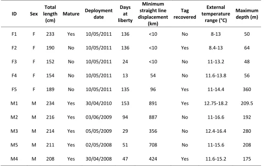
3.2.1 Tagging of sharks

Ten pop-up satellite archival tags (MK10 PSAT, Wildlife Computers, Redmond, WA, USA) were deployed on five male and five female broadnose sevengill sharks from 2008 to 2011 (Table 3.1). These tags measure external temperature, depth and light level at user-defined time intervals, detach from the animal after a pre-programmed deployment period and transmit the collected data to the Argos satellite system. Since satellite bandwidth is limited, depth and temperature data are summarized for a specified summary period as histograms of time spent at a set of depth and temperature bins and as temperature-at-depth profiles. Since tags were deployed over four years, data returns from initial tag releases informed the programming of subsequent tags to optimize sampling efficiency, resulting in different tag setups between years (Table 3.2).

(71)

70

carefully removed from the shark’s mouth, their eyes covered with a wet cloth to avoid injury, their sex identified and total length measured.

Tags were attached to the shark by implanting a stainless steel anchor, which was attached to the tag via a 100 mm long, nylon coated, multi-strand, stainless steel wire trace (2 mm

diameter) into the dorsal musculature. A second anchor with a stainless steel wire loop

attached to it, which was placed around the body of the tag, was implanted approximately 100 mm behind the first anchor to prevent excessive sideways movement of the PSAT. Aseptic techniques were used during anchor implantation and the entire procedure lasted

approximately 3-5 minutes. Running seawater was continuously pumped over the gills of the shark throughout the procedure. Prior to release, a povidone-iodine antiseptic was applied to the wounds to aid healing. All methods used were approved by the University of

Tasmania Animal Ethics Committee (Approval No A0011590).

3.2.2 Data analysis

Records from the first 24 hours of archival records were removed from the dataset to remove any abnormal behavior associated with tagging stress. Records following tag detachment were also removed from the dataset.