PP 2006 25: Intuitionistic Logic

Intuitionistic Logic

Nick Bezhanishvili and Dick de Jongh

Institute for Logic, Language and Computation

Universiteit van Amsterdam

Contents

1 Introduction 2

2 Intuitionism 3

3 Kripke models, Proof systems and Metatheorems 8

3.1 Other proof systems . . . 8

3.2 Arithmetic and analysis . . . 10

3.3 Kripke models . . . 15

3.4 The Disjunction Property, Admissible Rules . . . 20

3.5 Translations . . . 22

3.6 The Rieger-Nishimura Lattice and Ladder . . . 24

3.7 Complexity ofIPC. . . 25

3.8 Mezhirov’s game for IPC . . . 28

4 Heyting algebras 30 4.1 Lattices, distributive lattices and Heyting algebras . . . 30

4.2 The connection of Heyting algebras with Kripke frames and topologies . . . 33

4.3 Algebraic completeness ofIPCand its extensions . . . 38

4.4 The connection of Heyting and closure algebras . . . 40

5 Jankov formulas and intermediate logics 42 5.1 n-universal models . . . 42

5.2 Formulas characterizing point generated subsets . . . 44

5.3 The Jankov formulas . . . 46

5.4 Applications of Jankov formulas . . . 47

1

Introduction

In this course we give an introduction to intuitionistic logic. We concentrate on the propositional calculus mostly, make some minor excursions to the predicate calculus and to the use of intuitionistic logic in intuitionistic formal systems, in particular Heyting Arithmetic. We have chosen a selection of topics that show various sides of intuitionistic logic. In no way we strive for a complete overview in this short course. Even though we approach the subject for the most part only formally, it is good to have a general introduction to intuitionism. This we give in section 2 in which also natural deduction is introduced. For more extensive introductions see [35],[17].

After this introduction we start with other proof systems and the Kripke models that are used for intuitionistic logic. Completeness with respect to Kripke frames is proved. Metatheorems, mostly in the form of disjunction prop-erties and admissible rules, are explained. We then move to show how classical logic can be interpreted in intuitionistic logic by G¨odels’s negative translation and how in its turn intuitionistic logic can be interpreted by another translation due to G¨odel into the modal logic S4 and several other modal logics. Finally we introduce the infinite fragment of intutionistic logic of 1 propositional vari-able. The Kripke model called the Rieger-Nishimura Ladder that comes up while studying this fragment will play a role again later in the course. The next subject is a short subsection in which the complexity of the intuitionistic propositional calculus is shown to bePSPACE-complete. We end up with a discussion of a recently developed game for intuitionistic propositional logic [25]. In the next section Heyting algebras are discussed. We show the connec-tions with intuitionistic logic itself and also with Kripke frames and topology. Completeness ofIPCwith respect to Heyting algebras is shown. Unlike in the case of Kripke models this can straightforwardly be generalized to extensions ofIPC, the so-called intermediate logics. The topological connection leads also to closure algebras that again give a relation to the modal logic S4 and its extensionGrz.

2

Intuitionism

Intuitionism is one of the main points of view in the philosophy of mathematics, nowadays usually set oppositeformalism andPlatonism. As such intuitionism is best seen as a particular manner of implementing the idea ofconstructivism

in mathematics, a manner due to the Dutch mathematician Brouwer and his pupil Heyting. Constructivism is the point of view that mathematical objects exist only in so far they have been constructed and that proofs derive their validity from constructions; more in particular, existential assertions should be backed up byeffectiveconstructions of objects. Mathematical truths are rather seen as being created than discovered. Intuitionism fits into idealistic trends in philosophy: the mathematical objects constructed are to be thought of as idealized objects created by an idealized mathematician (IM), sometimes called

the creatingorthe creative subject. Often in its point of view intuitionism skirts the edges ofsolipsismwhen the idealized mathematician and the proponent of intuitionism seem to fuse.

Much more than formalism and Platonism, intuitionism is in principle nor-mative. Formalism and Platonism may propose a foundation for existing math-ematics, a reduction to logic (or set theory) in the case of Platonism, or a consistency proof in the case of formalism. Intuitionism in its stricter form leads to a reconstruction of mathematics: mathematics as it is, is in most cases not acceptable from an intuitionistic point of view and it should be attempted to rebuild it according to principles that are constructively acceptable. Typi-cally it is not acceptable to prove∃x φ(x) (for somex,φ(x) holds) by deriving a contradiction from the assumption that∀x¬φ(x) (for each x, φ(x) does not hold):reasoning by contradiction. Such a proof does not create the object that is supposed to exist.

Actually, in practice the intuitionistic point of view hasn’t lead to a large scale and continuous rebuilding of mathematics. For what has been done in this respect, see e.g. [4]. In fact, there is less of this kind of work going on now even than before. On the other hand, one might say that intuitionism describes a particular portion of mathematics, the constructive part, and that it has been described very adequately by now what the meaning of that constructive part is. This is connected with the fact that the intuitionistic point of view has been very fruitful inmetamathematics, the construction and study of systems in which parts of mathematics are formalized. After Heyting this has been pursued by Kleene, Kreisel and Troelstra (see for this, and an extensive treatment of most other subjects discussed here, and many other ones [35]). Heyting’s [17] will always remain a quickly readable but deep introduction to the intuitionistic ideas. In theoretical computer science many of the formal systems that are of foundational importance are formulated on the basis of intuitionistic logic.

Platonist ideas proposed by Frege, Russell and Hilbert. In particular, Poincar´e maintained in opposition to the formalists and Platonists that mathematical induction (over the natural numbers) cannot be reduced to a more primitive idea. However, from the start Brouwer was more radical, consistent and en-compassing than his predecessors. The most distinctive features of intuitionism are:

1. The use of a distinctive logic: intuitionistic logic. (Ordinary logic is then calledclassicallogic.)

2. Its construction of the continuum, the totality of the real numbers, by means ofchoice sequences.

Intuitionistic logic was introduced and axiomatized by A. Heyting, Brouwer’s main follower. The use of intuitionistic logic has most often been accepted by other proponents of constructive methods, but the construction of the contin-uum much less so. The particular construction of the contincontin-uum by means of choice sequences involves principles that contradict classical mathematics. Constructivists of other persuasion like the school of Bishop often satisfy themselves in trying to constructively prove theorems that have been proved in a classical manner, and shrink back from actually contradicting ordinary mathematics.

Intuitionistic logic. We will indicate the formal system of intuitionistic propo-sitional logic byIPCand intuitionistic predicate logic byIQC; the correspond-ing classical systems will be namedCPCandCQC. Formally the best way to characterize intuitionistic logic is by anatural deduction system `a la Gentzen. (For an extensive treatment of natural deduction and sequent systems, see [34].) In fact, natural deduction is more natural for intuitionistic logic than for classical logic. A natural deduction system hasintroduction rules andeliminationrules for the logical connectives ∧ (and), ∨ (or) and → (if ..., then) andquantifiers

∀(for all) and∃(for at least one). The rules for ∧, ∨ and → are:

• I∧: Fromφandψconcludeφ∧ψ,

• E∧: Fromφ∧ψconcludeφand conclude ψ,

• E→: Fromφandφ→ψconclude ψ,

• I→: If one has a derivation ofψfrom premiseφ, then one may conclude toφ→ψ(simultaneously dropping assumptionφ),

• I∨: Fromφconclude toφ∨ψ, and from ψconclude toφ∨ψ,

• E∨: If one has a derivation of χ from premise φ and a derivation of χ

from premise ψ, then one is allowed to conclude χ from premise φ∨ψ

(simultaneously dropping assumptionsφandψ),

• E∀: If one has a derivation of∀xφ(x), then on may concludeφ(t) for any termt,

• I∃: Fromφ(t) for any termtone may conclude∃xφ(x),

• E∃: If one has a derivation of ψfrom φ(x) in whichxis not free in in ψ

itself or in any premise other than φ(x), then one may conclude ψ from premise∃xφ(x), dropping the assumptionφ(x) simultaneously.

One usually takes negation¬(not) of a formulaφ to be defined asφimplying a contradiction (⊥). One adds then theex falso sequitur quodlibet rulethat

• anything can be derived from ⊥.

If one wants to get classical propositional or predicate logic one adds the rule that

• if⊥is derived from¬φ, then one can conclude toφ, simultaneously drop-ping the assumption¬φ.

Note that this is not a straightforward introduction or elimination rule as the other rules.

The natural deduction rules are strongly connected with the so-called BHK-interpretation (named after Brouwer, Heyting and Kolmogorov) of the con-nectives and quantifiers. This interpretation gives a very clear foundation of intuitionistically acceptable principles and makes intuitionistic logic one of the very few non-classical logics in which reasoning is clear, unambiguous and all encompassing but nevertheless very different from reasoning in classical logic.

In classical logic the meaning of theconnectives, i.e. the meaning of complex statements involving the connectives, is given by supplying thetruth conditions

for complex statements that involve the informal meaning of the same connec-tives. For example:

• φ∧ψis true if and only ifφis trueandψis true, • φ∨ψis true if and only ifφis trueorψis true, • ¬φis true iffφisnottrue

The BHK-interpretation of intuitionistic logic is based on the notion ofproof

instead of truth. (N.B!Notformal proof, or derivation, as in natural deduction or Hilbert type axiomatic systems, but intuitive (informal) proof, i.e. convincing mathematical argument.) The meaning of the connectives and quantifiers is then just as in classical logic explained by the informal meaning of their intuitive counterparts:

• A proof ofφ∨ψconsists of a proof ofφora proof ofψplus a conclusion φ∨ψ,

• A proof ofφ→ψconsists of a method of convertingany proof ofφinto a proof ofψ,

• Noproof of⊥exists,

• A proof of ∃x φ(x) consists of a named of an object constructed in the intended domain of discourse plus a proof of φ(d) and the conclusion ∃x φ(x),

• A proof of∀x φ(x) consists of a method thatfor anyobjectdconstructed in the intended domain of discourse produces a proof ofφ(d).

For negations this then means that a proof of¬φis a method of converting any supposed proof ofφ into a proof of a contradiction. That ⊥ →φ has a proof for anyφ is based on the intuitive counterpart of the ex falso principle. This may seem somewhat less natural then the other ideas, and Kolmogorov did not include it in his proposed rules.

Together with the fact that statements containing negations seem less con-tentful constructively this has lead Griss to consider doing completely without negation. Since however it is often possible to prove such more negative state-ments without being able to prove more positive counterparts this is not very attractive. Moreover, one can do without the formal introduction of⊥in natu-ral mathematical systems, because a statement like 1 = 0 can be seen to satisfy the desired properties of⊥without making any ex falso like assumptions. More precisely, not only statements for which this is obvious like 3 = 2, but all state-ments in those intuitionistic theories are derivable from 1 = 0 without the use of the rules concerning⊥. If one nevertheless objects to the ex falso rule, one can use the logic that arises without it, calledminimal logic.

The intuitionistic meaning of a disjunction is only superficially close to the classical meaning. To prove a disjunction one has to be able to prove one of its members. This makes it immediately clear that there is no general support forφ∨¬φ: there is no way to invariably guarantee a proof of φ or a proof of ¬φ. However, many of the laws of classical logic remain valid under the BHK-interpretation. Various decision methods for IPC are known, but it is often easy to decide intuitively:

• A disjunction is hard to prove: for example, of the four directions of the twode Morgan lawsonly¬(φ∧ψ)→ ¬φ∨¬ψis not valid, other examples of such invalid formulas are

– φ∨¬φ(the law of the excluded middle)

– (φ→ψ)→ ¬φ∨ψ

• An existential statement is hard to prove: for example, of the four direc-tions of the classically valid interacdirec-tions between negadirec-tions and quantifiers only¬ ∀x φ→ ∃x¬φis not valid,

• statements directly based on the two-valuednes of truth values are not valid, e.g.¬ ¬φ→φor ((φ→ψ)→φ)→φ(Peirce’s law), and contraposi-tionin the form (¬ψ→ ¬φ)→φ→ψ),

• On the other hand, many basic laws naturally remain valid, commutativity and associativity of conjunction and disjunction, both distributivity laws, and

– (φ→ψ∧χ)↔(φ→ψ)∧(φ→χ), – (φ→χ)∧(ψ→χ)↔((φ∨ψ)→χ)), – (φ→(ψ→χ))↔(φ∧ψ)→χ.

– (φ∨ψ)∧¬φ→ψ) (needs ex falso!),

– (φ→ψ)→((ψ→χ)→(φ→χ)),

– (φ→ψ)→(¬ψ→ ¬φ) (the converseform of contraposition), – φ→ ¬¬φ,

– ¬¬¬φ↔ ¬φ(triple negations are not needed).

Slightly less obvious is thatdouble negation shiftis valid for ∧ and → but not for∀, at least in one direction. Valid are:

• ¬ ¬(φ∧ψ)↔ ¬ ¬φ∧¬ ¬ψ,

• ¬ ¬(φ→ψ)↔ ¬ ¬φ→ ¬ ¬ψ,

• ¬ ¬∀xφ(x)→ ∀x¬ ¬φ(x) (but not its converse).

The BHK-interpretation was independently given by Kolmogorov and Heyting, with Kolmogorov’s formulation in terms of the solution of problems rather than in terms of executing proofs. Of course, both extracted the idea from Brouwer’s work. In any case, it is clear from the above that, if a logical schema is (formally) provable inIPC(say, by natural deduction), then any instance of the scheme will have an informal proof following the BHK-interpretation.

Clearly, in the most direct sense intuitionistic logic is weaker than classical logic. However, from a different point of view the opposite is true. By G¨odel’s so-callednegative translationclassical logic can be translated into intuitionistic logic. To translate a classical statement one puts ¬ ¬ in front of all atomic formulas and then replaces each subformula of the formφ∨ψ by¬(¬φ∧¬ψ) and each subformula of the form∃x φ(x) by¬ ∀x¬φ(x) in a recursive manner. The formula obtained is provable in intuitionistic logic exactly when the original one is provable in classical logic. Some examples are:

• (¬q→ ¬p)→(p→q) becomes (¬ ¬ ¬q→ ¬ ¬ ¬p)→(¬ ¬p→ ¬ ¬q), • ¬ ∀x Ax→ ∃x¬Axbecomes ¬ ∀x¬ ¬Ax→ ¬ ∀x¬ ¬Ax

Thus, one may say that intuitionistic logic accepts classical reasoning in a particular form and is therefore richer than classical logic.

3

Kripke models, Proof systems and

Metatheo-rems

3.1

Other proof systems

We start this section with a Hilbert type system for intuitionistic logic. We will call the intuitionistic propositional calculus IPC and the intuitionistic predicate calculus IQC in contrast to the classical systems CPC and CQC. For extensive information on the topics treated in this section, see [34].

Axioms for a Hilbert type system for IPC. 1. φ→(ψ→φ).

2. (φ→(ψ→χ))→((φ→ψ)→(φ→χ)). 3. φ∧ψ→φ.

4. φ∧ψ→ψ. 5. φ→φ∨ψ.

6. ψ→φ∨ψ.

7. (φ→χ)→((ψ→χ)→(φ∨ψ→χ)).

8. ⊥ →φ.

with the rule ofmodus ponens: fromφandφ→ψconcludeψ.

This system is closely related to the natural deduction system. The first two axiom schemes are exactly sufficient to prove the deduction theorem, which mirrors the introduction rule for implication.

Theorem 1. (Deduction Theorem )IfΓ, φ`IPCψ, thenΓ`IPCφ→ψ.

Proof. By induction on the length of the derivation, using the fact that χ→χ

is derivable. ¤

Gentzen sequent calculus for IPC. • Structural rules (like weakening),

• Axioms: Γ, φ,∆ =⇒Θ, φ,Λ and Γ,⊥,∆ =⇒Θ, • L∧

Γ, φ, ψ,∆ =⇒Θ Γ, φ∧ψ,∆ =⇒Θ, • R∧:

Γ =⇒∆, φ,Θ and Γ =⇒∆, ψ,Θ Γ =⇒∆, φ∧ψ,Θ,

• L∨:

Γ, φ,∆ =⇒Θ and Γ, ψ,∆ =⇒Θ Γ, φ∨ψ,∆ =⇒Θ,

• R∨:

Γ =⇒∆, φ, ψ,Θ Γ =⇒∆, φ∨ψ,Θ, • R→:

Γ, φ,∆ =⇒ψ

Γ,∆ =⇒Θ, φ→ψ,Λ, • L→:

Γ, ψ,∆ =⇒Θ and Γ, φ→ψ,∆ =⇒φ,Θ Γ, φ→ψ,∆ =⇒Θ,

• Cut

Γ =⇒∆, φandφ,Γ =⇒∆ Γ =⇒∆.

This, not very common, sequent calculus system for IPC has the advantage that, read from bottom to top these rules are rules for a semantic tableau

system forIPC. A more standard sequent calculus system forIPCis obtained by restricting in a sequent calculus for classical logic CPC the sequence of formulas on the right to one formula (or none). For example,R∨ becomes:

Γ =⇒φ

Γ =⇒φ∨ψ

Predicate calculus.

We give just the axioms for the Hilbert type system:

1. ∀x φ(x)→φ(t), withtnot containing variables that become bound inφ(t). 2. φ(t)→ ∃x φ(x), with t not containing x or variables that become bound

inφ(t).

and the rules:

3. Fromφ→ψ(x) concludeφ→ ∀x ψ(x), ifxnot free inφ. 4. Fromφ(x)→ψconclude ∃x φ(x)→ψ, ifxnot free inψ.

3.2

Arithmetic and analysis

Classical arithmetic of the natural numbers is formalized inPAby the so-called

Peano axioms(the idea of which is originally due to Dedekind). The axioms for intuitionistic arithmetic (orHeyting arithmetic)HA are the same:

These axioms can simply be added to the Hilbert system for the predicate calculus, or, for that matter to a natural deduction or sequent system. HA-models are simply predicate logic HA-models for the language ofHA in which the HA-axioms are verified at each node.

Arithmetic. Classical arithmetic of the natural numbers is formalized inPA by the so-calledPeano axioms(the idea of which is originally due to Dedekind). These axioms

• x+ 16= 0,

• x+ 1 =y+ 1→x=y, • x+ 0 =x,

• x+ (y+ 1) = (x+y) + 1, • x .0 = 0,

• x .(y+ 1) =x . y+x, and theinductionscheme

• For eachφ(x),φ(0)∧∀x(φ(x)→φ(x+ 1))→ ∀xφ(x).

inasmuch as one of the elements of the two-oneness maybe thought of as a new two-oneness, which process may be repeated indefinitely. . .”).

Worth while noting is that the scheme

• For eachφ(x),∃xφ(x)→ ∃x(φ(x)∧∀y<x¬φ(y))

is classically but not intuitionistically equivalent to the induction scheme. (Here

y<xis defined as∃z(y+ (z+ 1) =x).)

G¨odels’ negative translation is applicable to HA/PA. Of course, also G¨odel’s incompleteness theorem applies to HA: there exists a φ such that neither `HAφ, nor `HA¬φ, and thisφcan be taken to have the form∀xψ(x)

for someψ(x) such that, for eachn, `HAψ(¯n). (Here ¯nstands for 1 +. . .+ 1

withnones, a term with the valuen.)

Free choice sequences. A great difficulty in setting up constructive versions of mathematics is the continuum. It is not difficult to reason about individual real numbers via for example Cauchy sequences, but one loses that way the intuition of the totality of all real numbers which does seem to be a primary intuition. Brouwer based the continuum on the idea of choice sequences. For example, a choice sequenceαof natural numbers is viewed as an ever unfinished, ongoing process of choosing natural number values α(0), α(1), α(2),· · · by the ideal mathematician IM. At any stage of IM’s activity only finitely many values have been determined by IM, plus possibly some restrictions on future choices. This straightforwardly leads to the idea that a function f giving values to all choice sequences can do so only by having the value f(α) for any particular choice sequenceαdetermined by a finite initial segmentα(0), . . . , α(m) of that choice sequence, in the sense that all choice sequencesβ starting with the same initial segmentα(0), . . . , α(m) have to get the same value under the function:

f(β) =f(α). This idea will lead us to Brouwer’s theorem that every real function on a bounded closed interval is necessarily uniformly continuous. Of course, this is in clear contradiction with classical mathematics.

Before we get to a characteristic example of a less severe distinction between classical and intuitionistic mathematics, theintermediate value theorem, let us discuss the fact that counterexamples to classical theorems in logic or math-ematics can be given as weak counterexamples or strong counterexamples. A weak counterexample to a statement just shows that one cannot hope to prove that statement, a strong counterexample really derives a contradiction from the general application of the statement. For example, to give a weak counterexam-ple top∨¬pit suffices to give a statementφthat has not been proved or refuted, especially a statement of a kind that can always be reproduced if the original problems is solved after all. A strong counterexample toφ∨¬φcannot consist

of proving¬(φ∨¬φ) for some particularφ, since¬(φ∨¬φ) is even in

intuition-istic logic contradictory (it is directly equivalent to¬φ∧¬ ¬φ). But a predicate φ(x) in intuitionistic analysis can be found such that ¬ ∀x(φ(x)∨¬φ(x)) can

be proved, which can reasonably be called a strong counterexample.

π. For example consider the number a= 0, a0a1a2 . . . for which the decimal

expansion1 _{defined as follows:}

As long as no sequence 1234567890 has occurred in the decimal expansion ofπ,an is defined to be 3. If a sequence 1234567890 has occcurred in the dec-imal expansion ofπ starting at some m with m6n, then, if the first such m

is evenan is 0 for all n>m, if it is odd, am= 4 and an= 0 for all n>m. As long as the problem has not been solved whether such a sequence exists it is not known whether a<1₃ or a=1₃ or a>1₃. That this is time bound is shown by the fact that in the meantime this particular problem has been solved, m

does exist and is even, soa<1₃ [7]. But that does not matter, such problems can, of course, be multiplied endlessly, and (even though we don’t take the trouble to change our example) this shows that it is hopeless to try to prove that, for any a, a<1₃∨a=1₃∨a>1₃. Note that, also a cannot be shown to be rational, because for that, p andq should be given such that a=p_q, which clearly cannot be done without solving the problem. On the other hand, ob-viously,¬ ¬(a<1₃∨a=1₃∨a>1₃) does hold, ais not not rational. In any case, weak counterexamples are not mathematical theorems, but they do show which statements one should not try to prove. Later on, Brouwer used unsolved prob-lems to provide weak and strong counterexamples in a stronger way by making the decimal expansion ofadependent on the creating subjects’ insight whether he had solved a particular unsolved problem at the moment of the construc-tion of the decimal in quesconstruc-tion. Attempts to formalize these so-calledcreative subject argumentshave lead to great controversy and sometimes paradoxical con-sequences. For a reconstruction more congenial to Brouwer’s ideas that avoids such problematical consequences, see [26].

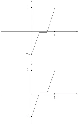
Let us now move to using a weak counterexample to show that one cannot hope to prove the so-calledintermediate value theorem. A continuous function

f that has value −1 at 0 and value 1 at 1 reaches the value 0 for some value between 0 and 1 according to classical mathematics. This does not hold in the constructive case: a functionf that moves linearly from value−1 at 0 to value

a− 1 3 at

1

3, stays at value a− 1 3 until

2

3 and then moves linearly to 1 cannot

be said to reach the value 0 at a particular place if one does not know whether

a>1₃, a=1 3 or a<

1

3. Since there is no method to settle the latter problem in

general, one cannot determine a valuexwheref(x) = 0. (See Figure 1.) Constructivists of the Russian school did not accept the intuitionistic con-struction of the continuum, but neither did they shrink from results contradict-ing classical mathematics. They obtained such results in a different manner however, by assuming that effective constructions are recursive constructions, and thus in particular when one restricts functions to effective functions that all functions are recursive functions. Thus, in opposition to the situation in classical mathematics, accepting the so-calledChurch-Turing thesisthat all

ef-1_{To make arguments easier to follow, we discuss these problems regarding real numbers}

−

1

1

1

−

1

1

1

fective functions are recursive does influence the validity of mathematical results directly.

Let us remark finally that, no matter what ones standpoint is, the resulting formalized intuitionistic analysis has a more complicated relationship to classical analysis than the one betweenHA and PA, the negative translation does no longer apply.

Realizability. Kleene used recursive functions in a different manner than the Russian constructivists. Starting in the 1940’s he attempted to give a faithful interpretation of intuitionistic logic and (formalized) mathematics by means of recursive functions. To understand this, we need to know two basic facts. The first is that there is a recursive way of coding pairs of natural numbers by a single one,j is a bijection from IN2 _{to IN: j(m, n) codes the pair (m, n) as a single}

natural number. Decoding is done by the functions ( )0 and ( )1: ifj(m.n) =p,

then (p)0=mand (p)1=n. The second insight is that all recursive functions,

or easier to think about, all the Turing machines that calculate them can be coded by natural numbers as well. Ifecodes a Turing machine, then{e}is the function that is calculated by it, i.e. for each natural numbern, {e}(n) has a certain value if on input nthe Turing machine coded bye delivers that value. Now Kleene defines how a natural number realizes an arithmetic statement (in the language ofHA):

• Anyn∈IN realizes an atomic sentence iff the statement is true, • nrealizesφ∧ψiff (n)0realizes φand (n)1 realizes ψ,

• nrealizesφ∨ψiff (n)0= 0 and (n)1realizesφ, or (n)0= 1 and (n)1realizes

ψ,

• nrealizesφ→ψiff, for anym∈IN that realizesφ,{n}(m) has a value that realizesψ,

• n realizes ∀xφ(x) iff, for each m∈IN, {n}(m) has a value that realizes

φ(m),

• nrealizes∃xφ(x) iff, (n)1 realizesφ((n)0).

Intuitionistic logic in intuitionistic formal systems. Intuitionistic logic, in the form of propositional logic or predicate logic satisfies the so-called dis-junction property: if φ∨ψ is derivable, then φis derivable or ψ. This is very characteristic for intuitionistic logic: for classical logic p∨¬pis an immediate counterexample to this assertion. The property also transfers to the usual for-mal systems for arithmetic and analysis. Of course, this is in harmony with the intuitionistic philosophy. Ifφ∨ψis formally provable, then if things are right it is informallly provable as well. But then, according to the BHK-interpretation,

φorψshould be provable informally as well. It would at least be nice if the for-mal system were complete enough to provide this forfor-mal proof, and in the usual case it does. For existential statements something similar holds, an existence property, if ∃x φ(x) is derivable in Heyting’s arithmetic, then φ(¯n) is derivable for some ¯n. Statements of the form∀y∃x φ(y, x) express the existence of func-tions, and, for example for Heyting’s arithmetic, the existence property then transforms in: if such a statements is derivable, then also some instantiation of it as a recursive function as was stated above already. In classical Peano arith-metic such properties only hold for particularly simple, e.g. quantifier-free,φ. In fact, with regard to the latter statements, classical and intuitionistic arithmetic are of the same strength.

Some formal systems may be decidable (e.g. some theories of order) and then one will have classical logic in most cases. However, in Heyting’s arithmetic one has de Jongh’s arithmetic completeness theorem stating that its logic is exactly the intuitionistic one: if a formula is not derivable in intuitionistic logic an arithmetic substitution instance can be found that is not derivable in Heyting’s arithmetic (see e.g. [21], [32]). For the particular case ofp∨¬p this

is easy to see, it follows immediately from G¨odel’s incompleteness theorem and the disjunction property: by G¨odel a sentence φexists whichHA can neither prove nor refute, by the disjunction propertyHAwill then not be able to prove

φ∨¬φeither.

3.3

Kripke models

Definition 3. A KripkeframeK= (K, R)forIPChas a reflexive partial order

R. A Kripke model (K, R, V) for IPC on such a frame is persistent, in the sense that, ifwRw0 _andw

∈V(p), thenw0∈V(p). The rules forforcingof the formulas are:

1. w²piffw∈V(p),

2. w²φ∧ψ iffw²φandw²ψ,

3. w²φ∨ψ iffw²φorw²ψ,

4. w²φ→ψiff, for allw0 _{such thatwRw}0_{, ifw}0_{²φ, thenw}0_²ψ,

p

(a)

p, q

p, r

(b)

q

r

p

(c)

p

(d)

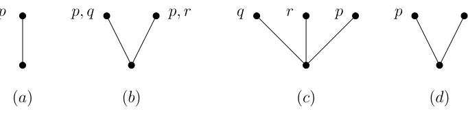
Figure 2: Counter-models for the propositional formulas

Most of our Kripke models will berootedmodels, they have a least node (often

w0), aroot. For the predicate calculus each nodewof a model is equipped with

a domainDw in such a way that, if wRw0, thenDw⊆Dw0. Persistency comes

in this case down to the fact thatDw is a submodel ofDw0 in the normal sense

of the word. The clauses for the quantifiers are (adding names for the elements of the domain to the language):

1. w²∃xφ(x) iff, for somed∈Dw, w²φ(d). 2. w²∀xφ(x) iff, for eachw0 _withwRw0 _{and alld}

∈D_w0,w0²φ(d).

HA-models are simply predicate-logic models for the language ofHAin which theHA-axioms are verified at each node.

Persistency transfers to formulas: ifwRw0 _andw

²φ, thenw0

²φ. Exercise 4. Prove that persistency transfers to formulas.

It is helpful to note that w²¬¬φ iff, for each w0 _{such that wRw}0_{, there}

existsw00_withw0_Rw00_withw00_{²φ. For finite models this simplifies tow²¬¬φ}

iff for all maximal nodesw0 _{above w,w}0_²φ.

Theorem 5. (Glivenko) `CPCφiff `IPC¬ ¬φ.

Exercise 6. Show Glivenko’s Theorem in two ways. First, by using one of the proof systems. Secondly, assuming the completeness theorem with respect to finite Kripke models.

We will see shortly that this does not extend to the predicate calculus or arithmetic.

The following models invalidate respectively p∨¬p, ¬¬p→p (both

Fig-ure 2a), (¬¬p→p)→p∨¬p) (Figure 2d), (p→q∨r)→(p→q)∨(p→r)

(Fig-ure 2b), (¬p→q∨r)→(¬p→q)∨(¬p→r) (Figure 2c),¬¬∀x(Ax∨¬Ax)

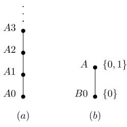
(Fig-ure 3a, constant domain IN),∀x(A∨Bx)→A∨∀xBx (Figure 3b).

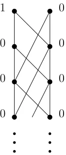
A0

A1

A2

A3 ..

. .

(a)

B0

A

{0} {0,1}

(b)

Figure 3: Counter-models for the predicate formulas

Definition 8.

1. If F= (W, R) is a frame and w∈W, then the generated subframe F_w is (R(w), R0_{), where R(w) ={w}0

∈W|wRw0} andR0 the restriction of R to

R(w). If Kis a model onF, then thegenerated submodel Kw is obtained

by restricting the forcing on Fw toR(w).

2. (a) If F= (W, R) and F0_{= (W}0_{, R}0_{) are frames, then f: W→W}0 _{is a}

p-morphism (alsobounded morphism)from FtoF0 _iff

i. for eachw, w0

∈W, if wRw0, thenf(w)Rf(w0),

ii. for eachw∈W, w0∈W0, if f(w)Rw0, then there exists w00∈W,

wRw00_andf(w00_{) =w}0_.

(b) If K= (W, R, V) and K0

= (W0 , R0

, V0

) are models, then f: W→W0

is a p-morhism from K to K0

iff f is a p-morhism of the respective frames and, for allw∈W,w∈V(p)ifff(w)∈V0(p).

3. If F1= (W1, R1) andF2= (W2, R2), then their disjoint unionF1]F2 has

as its set of worlds the disjoint union of W1 and W2, and R is R1∪R2.

To obtain the disjoint union of two models the union of the two valuations is added.

Theorem 9.

1. If w0 _{is a node in the generated submodel}

Mw, then, for eachφ,w0²φin

Miffw0

²φin Mw.

2. If f is a p-morphism fromMtoM0 _andw

∈W, then, for eachφ,w²φiff

f(w)²φ.

3. If w∈W₁, thenw²φin M₁]M₂ iffw²φ inM₁, etc.

The method of canonical models used in modal logic can be adapted to the case of intuitionistic logic. Instead of considering maximal consistent sets of formulas we consider theories with the disjunction property.

Definition 10. A theory is a set of formulas that is closed under IPC -consequence. A set of formulasΓ has the disjunction property if φ∨ψ∈Γ

im-pliesφ∈Γor ψ∈Γ.

The Lindenbaum type lemma that is then needed is the following.

Lemma 11. If Γ₀IPCψ→χ, then a theory with the disjunction property ∆

that includesΓexists such that ψ∈∆ andχ∈/∆.

Proof. Enumerate all formulas: φ0, φ1,· · · and ddefine

• ∆0= Γ∪ {ψ},

• ∆n+1= ∆n∪ {φn} if this does not proveχ, • ∆n+1= ∆n otherwise.

Take ∆ to be the union of all ∆n. As in the usual Lindenbaum construction ∆ is a theory and none of the ∆nor ∆ itself proveχ. χsimply takes the place that ⊥has in classical proofs. Claim is that ∆ also has the the disjunction property and therefore satisfies all the desired properties. Assume that φ∨ψ∈∆, and

φ∈/∆, ψ∈/∆. Let φ=φ_m and ψ=φ_n and w.l.o.g. let n be the larger of m, n. Then χ is provable in both ∆n∪ {φ} and ∆n∪ {ψ} and thus in ∆n∪ {φ∨ψ} as well. But that cannot be true since ∆n∪ {φ∨ψ}⊆_{∆ and ∆0IPCχ.} ¤

Definition 12. (Canonical model)The canonical model ofIPCis a Kripke model based on a frameFC _{= (W}C_{, R}C_{), whereW}C _{is the set of all consistent}

theories with the disjunction property andRC _{is the inclusion. The canonical}

valuation onFC _{is defined by putting: Γ²pif p∈Γ.}

Theorem 13. (Completeness theorem for IQC, IPC) `IQC, IPCφ iffφ

is valid in all Kripke models for IQC, IPC (for IPC the finite models are sufficient).

Proof. We give the proof forIPCand make some comments aboutIQC. As in modal logic the proof proceeds by showing by induction on the length ofφthat Γ²φiffφ∈Γ. The only interesting case is the step of showing that, if

ψ→χ∈/Γ, then a theory with the disjunction property ∆ that includes Γ exists such thatψ∈∆ andχ∈/∆. This is the content of Lemma 11.

Finally, assume Γ₀IPCχ. Then Γ0IPC> →χ, so, again applying the

Lin-denbaum Lemma an extension ∆ of Γ with the disjunction property, not con-tainingχ , exists. In the canonical model, ∆₂χ.

Thefinite model propertyfor IPC(i.e. if 0IPCφ, then there exists a finite

contains all relevant formulas. Another way of doing this is usingfiltration. This works exactly as in modal logic.

The Henkin type proof for IQC is only slightly more complicated than a combination of the above proof and the proof for the classical predicate calculus. Of course, one needs the theories to have not only the disjunction property but also the existence property: if∃xφ(x)∈Γ then φ(d)∈Γ for some

d in the language of Γ. Since one needs growing domains one needs theories in different languages. Let C0, C1, C2,· · · be a sequence of disjoint countably

infinite sets of new constants. It suffices to consider theories in the languages obtained by adding C0∪C1· · · ∪Cn to the original language. For students who know the classical proof this turns then into a largerexercise (see [35],

Volume 1). ¤

Remark 14. If we restrict the propositional language to only finitely many variables, we obtain finite variable canonical models. These models provide completeness for finite variable fragments ofIPCand will come up later on in the study ofn-universal models.

Exercise 15. Prove, using an adequate set, the finite model property forIPC. When one adds schemes to the Hilbert type system ofIPCone obtains so-calledintermediate(orsuperintuitionistic) logics. For example addingφ∨¬φ, or

¬¬φ→φ or ((φ→ψ)→φ)→φ(Peirce’s law) one obtains classical logicCPC. Other well-known intermediate logics are:

• LC (Dummett’s logic) axiomatized by (φ→ψ)∨(ψ→φ). LC char-acterizes the linear frames and is complete with regard to the finite ones. Equivalent axiomatizations are (φ→ψ∨χ)→(φ→ψ)∨(φ→χ) or ((φ→ψ)→ψ)→φ∨ψ.

• KC (logic of the weak excluded middle), axiomatized by¬φ∨ ¬¬φ, com-plete with regard to the finite frames with a largest element.

• ((χ→(((φ→ψ)→φ)→φ))→χ)→χ (3-Peirce) characterizes the frames with depth 2 and is complete with regard to the finite ones.

• ∀x(φ∨ψx)→φ∨∀xψx is a predicate intermediate logic sound and

com-plete for the frames with constant domains.

Information on propositional intermediate logics can be found in [11]. Exercise 16. 1. Show the different axiomatizations ofLCto be equivalent.

2. Show that inKCit is sufficient to assume the axioms for atomic formulas. 3. Give a counterexample to “3-Peirce” on the linear frame of 3 elements. Formulate a conjecture for the logic that is complete with regard to frames of depthn.

4. Show that ∀x(φ∨ψx)→φ∨∀xψx is valid on frames with a constant

K L

w0

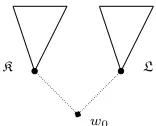
Figure 4: Proving the disjunction property

3.4

The Disjunction Property, Admissible Rules

Theorem 17. `IPCφ∨ψiff `IPCφ or `IPCψ. (This extends to the

predi-cate calculus and arithmetic.)

Proof. The idea of the nontrivial direction of the proof for IPC is to equip two supposed counter-models K and L for φ and ψ respectively, with a new root w0. In w0, φ∨ψ is falsified (see Figure 4 ). It is in the present case

not relevant how the forcing of the new root is defined as long as it is in line with persistency. In the case of arithmetic this method works also, but only for some models at the new root and it is difficult to prove, except when one uses for the new root the standard model IN. That the latter is always possible is known as (Smory´nski’s trick). We will return to it presently.¤

We callHA-models simply predicate logic models for the language ofHAin which theHA-axioms are verified at each node. By the (strong) completeness theorem the sentences true on all these models are the ones derivable fromHA. Lemma 18. In each node of each HA-model there exists in the domainDw of

each worldwa unique sequence of distinct elements that are the interpretations of thenumerals 0,1,· · ·, n,· · ·, wheren=S· · ·S

| {z }

n times 0

Proof. Straightforward from the axioms. ¤

Theorem 19. (Smory´nski’s trick)IfΣis a set ofHA-models, then a newHA -model is obtained by taking the disjoint union ofΣadding a new root w0 below

it and takingIN as its domainDw0.

Proof. The only thing to show is that the HA-axioms hold at w0. This is

obvious for the simple universal axioms. Remains to prove it for the induction axioms. Assumew0²φ(0) andw0²∀x(φ(x)→φ(Sx)). By using an (intuitive)

induction one sees that, for each n∈IN, w₀²φ(n). w₀²∀xφ(x) immediately follows because no problems can arise at nodes other thanw0. ¤

Corollary 20. `HAφ∨ψ iff `HAφor `HAψ.

Definition 21. (Aczel slash)

1. Γ|piffΓ`p,

2. Γ|φ∧ψ iffΓ|φ andΓ|ψ, 3. Γ|φ∨ψ iffΓ|φ orΓ|ψ,

4. Γ|φ→ψ iffΓ`φ→ψ and(notΓ|φ orΓ|ψ).

Can be extended to predicate calculus and arithmetic. Theorem 22. If Γ`φandΓ|χfor each χ∈Γ, thenΓ|φ.

This theorem is proved by induction on the length of the derivation in one of the proof systems.

Corollary 23.

1. χ|χiff, for allφ, ψ, if `IPCχ→φ∨ψ, then `IPCχ→φor `IPCχ→ψ.

2. If `IPC¬χ→φ∨ψ, then `IPC¬χ→φor `IPC¬χ→ψ.

3. χ|χ iff, for all rootedM, M0_{, if}

M²χandM0

²χ, thenN²χexists such that MandM0 _{are generated subframes of}

N.

This theorem can be read as a rule ¬χ→φ∨ψ/¬(χ→φ)∨(¬χ→ψ) that can be applied toIPCeven though the rule does not follow directly fromIPC. That such rules exist is very characteristic for intuitionistic systems.

Definition 24. An admissible ruleis a schematic rule of the form:

φ(χ1, . . . , χk)/ψ(χ1, . . . , χk)withφ andψparticular formulas and the property

that, for allIPC-formulasχ1, . . . , χk, if `IPCφ(χ1, . . . , χk), then

`IPCψ(χ1, . . . , χk).

Example 25. Admissible rules that do not correspond to derivable formulas of

IPCare for example:

1. ¬χ→φ∨ψ/(¬χ→φ)∨(¬χ→ψ), 2. gn(φ)/¬ ¬φ∨(¬ ¬φ→φ).

The second of these rules will occur in section 3.6.

Theorem 26. (R. Iemhoff) All admissible rules can be obtained using only derivability inIPCfrom the rules

η→φ∨ψ/(η→χ1)∨· · ·∨(η→χk)∨(η→φ)∨(η→ψ),

whereη= (χ1→δ1)∧· · ·∧(χk→δk).

We conclude this section with another application of Smory´nski’s trick: prov-ing arithmetic completeness (de Jongh’s theorem).

Theorem 28. (Arithmetic Completeness) `IPCφ(p1, . . . , pm)iff, for all

arithmetic sentencesψ1, . . . , ψm, `HAφ(ψ1, . . . , ψm).

Proof. (sketch). Assume 0IPCφ(p1,· · ·, pm) (the other direction being trivial).

A finite Kripke model on a frame F exists in which φ(p1,· · ·, pk) is falsified

in the root. By a standard procedure we can also assume that the frame is ordered as a tree, which at each node (except the maximal ones) has at least a binary split. The purpose of the latter is to ensure that each node is uniquely characterized by the maximal elements above it. Assume that w1,· · ·, wk are the maximal nodes of the tree. Using arithmetic considerations one can construct arithmetic sentences α1,· · ·, αk and PA-models M1,· · ·,Mk such that Mi²αj iff i=j. Noting that the one-node models Mi are immediately HA-models as well one now applies Smory´nski’s trick repeatedly to fill out the model by assigning IN to each node. One so obtains anHA-model onF. Next one notes that for each node w, the sentence ψw=¬¬(αi1∨· · ·∨αim),

wherewi1,· · ·, wim are the maximal elements that are successors ofwis forced at w and its successors and nowhere else. Finally taking each ψi to be the disjunction of thoseψw where pi is forced one sees that theψi behave in the HA-model exactly like the pi in the original Kripke model and thus one gets thatφ(ψ1,· · ·, ψm) is falsified in theHA-model and hence cannot be a theorem

ofHA. ¤

For a full version of this proof and more information on the application of Kripke models to arithmetical systems, see Sm73.

3.5

Translations

First we give G¨odel’s so-called negative translation of classical logic into intu-itionistic logic.

Definition 29.

1. pn_{=¬ ¬p,}

2. (φ∧ψ)n_=φn_∧ψn_,

3. (φ∨ψ)n=¬ ¬(φn∨ψn),

4. (φ→ψ)n_=φn_→ψn_,

5. ⊥n_=⊥.

There are many variants of this definition that give the same result. Theorem 30. `CPCφ iff `IPCφn. (This extends to the predicate calculus

Proof. for the propositional calculus.

⇐= : Of course, `CPCψ↔ψn. Also, if `IPCφ, then `CPCφ. Thus, this

direction follows.

=⇒: One first proves, by induction on the length ofφ, that `IPCφn↔ ¬ ¬φn

(φn _{is negative). This is straightforward; for the case of implication one uses} that `IPC¬¬(φ→ψ)↔(¬¬φ→ ¬¬ψ), and for conjunction the analogous

fact for ∧. Then, one proves, by induction on the length of the proof in the Hilbert type system that, if `CPCφ, then `IPCφn. In some cases one needs

the fact first proved thatχn _{is a negative formula, e.g. in the axiom ¬¬φ→φ}

that is added toIPCto obtainCPC. ¤

If one uses in the above proof the natural deduction system or a Gentzen system one automatically gets the slightly stronger result that Γ`CPCφ iff

Γn_`

IPCφn.

Exercise 31. Give a translation satisfying Theorem 30 that uses ∧ and¬only. Exercise 32. Prove Glivenko’s theorem using the G¨odel translation.

The propositional modal-logical systems S4,Grz and GLare obtained by adding to the axiom ¤(φ→ψ)→(¤φ→¤ψ) of the modal logic K, the ax-ioms ¤φ→φ, ¤φ→¤ ¤φ for S4, in addition to this Grzegorczyk’s axiom ¤(¤(φ→¤φ)→φ)→φforGrz, and¤(¤φ→φ)→¤φforGL. Completeness holds forS4with respect to the finite reflexive, transitive Kripke models, forGrz with respect to the finite partial orders (reflexive, transitive, anti-symmetric), and for GL with respect to the finite transitive, conversely well-founded (i.e. irreflexive) Kripke models.

Of course, one may note the closeness of IPC and Grz or S4 when one thinks of intuitionistic implication as necessary (’strict’) implication and no-tices the resemblance of the models. G¨odel saw the connection long before the existence of Kripke models by noting that interpreting¤ as the intuitive notion of provability the S4-axioms ¤(φ→ψ)→(¤φ→¤ψ), ¤φ→φ, ¤φ→¤ ¤φ

as well as its rule of necessitationφ/¤φbecome plausible. He constructed the following translation fromIPCintoS4.

Definition 33. G¨odel translation

1. p¤_=¤p,

2. (φ∧ψ)¤_=φ¤_∧ψ¤_,

3. (φ∨ψ)¤=φ¤∨ψ¤,

4. (φ→ψ)¤_=¤(φ¤_→ψ¤_),

Theorem 34. `IPCφ iff `S4φ¤ iff `Grzφ¤.

⇐= : It is sufficient to note that it is easily provable by induction on the length of the formula φ that for any world w in a Kripke model with a persistent valuation w²φ iff w²φ¤ _{(where on the left the forcing is interpreted in the}

intuitionistic manner and on the right in the modal manner). This means that if 0IPCφone can interpret the finiteIPC-counter model toφprovided by the

completeness theorem immediately as a finiteGrz-counter model toφ¤_{. ¤}

A natural adaptation of G¨odel’s translation can be given from IPC into provability logic GL when one notes that Grz-models and GL-models only differ in the fact thatGLhas irreflexive instead of reflexive models.

Definition 35.

1. p¡_=¤p∧p,

2. ⊥¡_=⊥,

3. (φ∧ψ)¡=φ¡∧ψ¡, 4. (φ∨ψ)¡_=φ¡_∨ψ¡_,

5. (φ→ψ)¡_=¤(φ¡_→ψ¡_)∧(φ¡_→ψ¡_),

Theorem 36. `IPCφ iff `GLφ¡.

3.6

The Rieger-Nishimura Lattice and Ladder

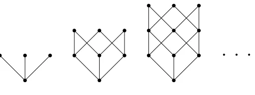
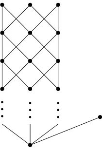
This section will introduce the fragment ofIPC of one propositional variable. We will see later that this is essentially the same as the free Heyting algebra on one generator. It is known under the name of the people who discovered it: Rieger [29] and Nishimura [27]. It is accompanied by a universal Kripke model: the Rieger-Nishimura Ladder.

Definition 37. (Rieger-Nishimura Lattice)

1. g0(φ) =f0(φ) =defφ,

2. g1(φ) =f1(φ) =def¬φ,

3. g2(φ) =def¬ ¬φ,

4. g3(φ) =def¬ ¬φ→φ,

5. gn+4(φ) =defgn+3(φ)→gn(φ)∨gn+1(φ),

6. fn+2(φ) =defgn(φ)∨gn+1(φ).

Theorem 38. Each formulaφ(p)with only the propositional variablepisIPC -equivalent to a formulafn(p) (n>2)orgn(p) (n>0) or>or⊥. All formulas

fn(p) (n>2) andgn(p) (n>0)are nonequivalent inIPC. In fact, in the

t t t @ @ @ @ @ @ ¡ ¡ ¡¡¡ ⊥ ¬p p

p∨¬p

¬¬p

¬¬p→p

¬p∨¬¬p

p→p

g4(p) f4(p)

t t t t ¡¡ ¡¡ ¡ @ @ @ @ @ @ @ @ @ ¡¡¡ t t t t ¡¡ ¡¡ ¡ @ @ @ @ @ @ @ @ @ ¡¡¡ t t t t ¡¡ ¡¡ ¡ @ @ @ @ @ @ @ @ @ ¡¡ ¡¡ ¡ t t t t t t t t t t t t t t t t t H H H H H H H H H H H H H H H H H H H H H H H H H H H H H H H H H H H H H H H H ¡ ¡ ¡ ¡ ¡ ¡ ¡ ¡ ¡ ¡ ¡ ¡ ¡ ¡ ¡ ¡ ¡ ¡ ¡ ¡ ¡ ¡ ¡ ¡ ¡ ¡ ¡ ¡ ¡ ¡ ¡ ¡ ¡ ¡ ¡ ¡ ¡ ¡ ¡ ¡

p w0 w1

w2 w3

Rieger-Nishimura Lattice (left) and Rieger-Nishimura Ladder (right)

In the Rieger-Nishimura lattice a formulaφ(p) impliesψ(p) inIPCiffψ(p) can be reached fromφ(p) by a downward going line.

Exercise 39. Check that in the Rieger-Nishimura Ladder wi validates gn(p) fori>nonly.

Theorem 40. ([21])If `IPCgn(φ)for any n∈IN, then `_IPC¬ ¬φor `IPC¬ ¬φ→φ. (Can be extended to arithmetic.)

Proof. (Harder)Exercise. ¤

3.7

Complexity of IPC

We reduce quantified Boolean propositional logic QBF, known to be PSPACE-complete, toIPC.QBFis an extension ofCPCin which the propo-sitional quantifiers can be thought of as ranging over the set of truth values {0,1}. Consider theQBF-formula

A=Qmpm· · ·Q1p1B(p1,· · ·, pm)

with B quantifier-free. We write • →p forp1,· · ·, pm

• →q forq1,· · ·, qm • j→pforp1,· · ·, pj−1

• j→qforq1,· · ·, qj−1

• p→j forpj+1,· · ·, pm,

• q→j forqj+1,· · ·, qm,

• Aj for

→ Q pj,

→

pj(p1,· · ·, pm)

We constructAj (linearly inA) by recursion onj:

A0(

→

p) =¬B(→p).

Aj(j→p, pj,

→ pj,

→

jq) = (pj∨¬pj)→Aj−1(

→

jp, pj,

→ pj,

→

jq) ifQj is∃, and

Aj(j→p, pj,

→ pj, qj,

→

jq) = (Aj−1→qj)→(pj→qj)∨(¬pj→qj) ifQj is∀.

ClaimFor any valuationv on→p:

v²Aj(p→j)⇐⇒ ∃M∃w∈M(w2Aj(

→

jp, pj,

→ pj,

→

q) &M(p→j) =v(p→j)),

whereM(p→j) =v(p→j) means that all nodes ofMvaluatep→j asv does. Proof of Claim. By induction on j

j= 0. =⇒: Takew to be the unique node of the Kripke model corresponding to the valuationv.

Qj=∃ =⇒: Assumev²∃pjAj−1(pj,

→

pj). Then, for somev0_{obtained fromvby}

adding a value forpj,v0_²A

j−1(pj,

→

pj). By the induction hypothesis,w0_{exists in}

some Kripke model M withM(pj,

→ pj) =v0_(p

j,

→

pj) andw02Aj−1(

→

jp, pj,

→ pj,

→

jq). Sincew0

²pj∨¬pj,w02pj∨¬pj→Aj−1=Aj, and soM, w0 satisfy the require-ments forw.

⇐= : Assume forw,MwithM(p→j) =v(

→ pj),

w2((pj∨¬pj)→Aj−1(

→

jp, pj,

→ pj,

→ q)).

Since the valuation of thep→jis constant we can assume w.l.o.g. thatw²pj∨¬pj andw2Aj−1(

→

jp, pj,

→ pj,

→

q)). Add the valuation ofpj inwtovto obtainv0. We then haveMw(pj

→

pj) =v0(pj,

→

pj). By the induction hypothesis for all valuations, so also forv0_,v0_²A

j−1(pj,

→

pj). Hence, v²∃pjAj−1(pj,

→ pj) .

Qj=∀ =⇒: Assume v²∀pjAj−1(pj,

→

pj). Then, for both ways, v0 and v1,

of extending v, vi²Aj−1(pj,

→

pj). By the induction hypothesis, we can find models Mi, with respective roots wi and Mi(pj,

→

pj) =vi(pj,

→

pj), such that

wi2Aj−1(

→

jp, pj,

→ pj,

→

jq)). Note that w0²pj, w1²¬pj. Add below the disjoint union of those two models a new rootw. The p→j is valued on was onw1 and

w2, the

→ p pj,

→

jqin conformity with persistency;qjis forced precisely whereAj−1

is forced. Thus Aj−1→qj is forced in M, andpj→qj and ¬pj→qj are not:

w2Aj.

⇐= : AssumeMand its rootware such thatM(p→j) =v(p→j) and

w2(Aj−1→qj)→(pj→qj)∨(¬pj→qj). There existw0,w1>wsuch that

• w0²¬pj,

• w02Aj−1(

→

jp, pj,

→ pj,

→

jq), • w1²pj,

• w12Aj−1(

→

jp, pj,

→ pj,

→

jq),

Let v0, v1 be the extensions of v with v0 satisfying ¬pj and v1 satisfying pj.

ClearlyMwi(pj,

→

pj) =vi(pj,

→

pj) in both cases. So, by the induction hypothesis, in both cases,vi²Aj−1(pj,

→

pj). Hence,v²∀pjAj−1(pj,

→ pj).

The final conclusion is that the mapping fromAtoAmis the desired reduc-tion. For the universal case (p→Aj−1)∨(¬p→Aj−1) would have worked as well

3.8

Mezhirov’s game for IPC

. We like to end up with something that has recently been developed: a game that is sound and complete for intuitionistic propositional logic announced in [25]. The games played are φ-gameswith φ being a formula of the propo-sitional calculus. The game has two playersP (proponent) and O (opponent). The playing field is the set of subformulas ofφ. A moveof a player is marking

a formula that has not been marked before. OnlyO is allowed to mark atoms. The first move is made byP, and consists of markingφ. Players do not move in turn; whose move it is is determined by thestate of the game. The player who has to move in a state where no move is availableloses. The state of the game is determined by the markings and by a classical valuationV al that is developed along with the markings. The rules for this valuation are at each stage

• for atoms thatV al(p) = 1 iffpis marked,

• for complex formulasψ◦χthat, ifψ◦χis unmarked,V al(ψ◦χ) = 0, and ifψ◦χis marked,V al(ψ◦χ) =V al(ψ)◦BV al(χ) where◦Bis the Boolean function associated with◦.

If a player has marked a formula that gets the valuation 0, then that is considered to be afault by that player. If P has a fault andO doesn’t thenP moves, in all other cases (i.e. ifO has fault andP does or doesn’t, or if neither player has a fault)O moves. The completeness theorem can be stated as follows.

Theorem 41. `IPCφiffP has a winning strategy in theφ-game.

We will first prove

Theorem 42. If 0IPCφ, then O has a winning strategy in theφ-game.

Proof. We write the sequences of formulas marked by O andP respectively as O and P. O keeps in mind a minimal counter-model for φ, i.e., in the root

w0, φ is not satisfied, but in all other nodes of the model φis satisfied. The

strategy of O is as follows. As long as P does not choose formulas false in nodes higher up in the model O just picks formulas that are true in w0. As

soon asP does choose a formula ψthat is falsified at a higher up in the model,

O keeps in mind the submodel generated by a maximal node w that falsifies

ψ. Okeeps repeating the same tactic with respect to the node where the game has lead the players. It is sufficient to prove the following:

Claim. If there are no formulas left for O to choose when following this strategy, i.e. all formulas that are true in thewthat is fixed in O’s mind have been marked, then it isP’s move.

Proof of Claim. We write|θ|w for the truth value of θ in w. As we will see it is sufficient to show that, if the situation in the game is as in the assump-tions of the claim, then |θ|w=V al(θ) for all θ. We prove, by induction onθ, |θ|w= 1⇐⇒V al(θ) = 1.

• Ifθ is atomic, thenO has marked all the atoms that are forced in wand no other, so those have become true and no other.

• Induction step ⇒: Assume |θ◦ψ|w= 1. Then θ◦ψ is marked, because otherwiseOcould do so, contrary to assumption. We have|θ|w◦B|ψ|w= 1. By IH,V al(θ)◦BV al(ψ) = 1, soV al(θ◦ψ) = 1.

• Induction step ⇐:

• V al(θ∧ψ) = 1⇒V al(θ) = 1 andV al(ψ) = 1⇒IH |θ|w= 1 and|ψ|w= 1⇒ |θ∧ψ|w= 1.

• ∨ is same as ∧.

• V al(θ→ψ) = 1⇒V al(θ) = 0 or V al(ψ) = 1, and thus by IH, |θ|w= 0 or |ψ|w= 1. Also, θ→ψ is marked, hence in O or P. In the first case |θ→ψ|w= 1 immediate, in the second, |θ→ψ|s= 1 for all s>w (P has marked no formulas false higher up, otherwise O would have shifted at-tention another node) and hence|θ|s= 0 or|ψ|s= 1 for alls>w. Indeed, |θ→ψ|w= 1.

We are now faced with the fact that O has only chosen formulas true in the world inO’s mind and those stay true higher up in the model. So,V al(θ) = 1 for allθ∈O. On the other hand,Phas at least one fault, the formulaξchosen byP that landed the game inwin the first place: V al(ξ) = 0. Indeed, it isP’s move.¤

We now turn to the second half:

Theorem 43. If `IPCφ, then P has a winning strategy in theφ-game.

Proof. P’s strategy is to choose only formulas that are provable fromO. Note thatP’s first forced choice of φis in line with this strategy. For this case it is sufficient to prove the following claim.

ClaimIf all formulas that are provable fromOare marked, then it isO’s move.

This is sufficient because it means that in such a situationOcan only mark a completely new formula, and when there are no such formulas left loses.

Proof of Claim. Create a model in the following manner. Assume χ1, . . . , χk are the formulas unprovable fromOand hence the unmarked ones. By the com-pleteness ofIPCthere arekmodels makingO true and falsifying respectively

• Atoms are forced inriff marked byO and then haveV al 1, otherwise 0. • Induction step ⇒: Assume|θ◦ψ|r= 1. Thenθ◦ψis marked, because if it wasn’t it would be one of the χi, falsifying persistency. We can reason on as in the other direction.

• Induction step ⇐:

• ∨ and ∧ as in the other direction.

• V al(θ→ψ) = 1⇒V al(θ) = 0 or V al(ψ) = 1, and thus by IH, |θ|r= 0 or |ψ|r= 1. Also,θ→ψis marked, hence inOorP, and so|θ→ψ|s= 1 and hence|θ|s= 0 or|ψ|s= 1 for all s>r. Indeed, |θ→ψ|r= 1.

We are now faced with the fact thatP has only marked formulas provable from Oand those will remain provable from O. So, V al(θ) = 1 for all θ∈P. So, P has no fault. By the rules of the game it isO’s move. ¤

4

Heyting algebras

4.1

Lattices, distributive lattices and Heyting algebras

We begin by introducing some basic notions. A partially ordered set (A,≤) is called alatticeif every two element subset ofAhas a least upper and greatest lower bound. Let (A,≤) be a lattice. For a, b ∈A let a∨b :=sup{a, b} and

a∧b:=inf{a, b}. We assume that every lattice is bounded, i.e., it has a least and a greatest element denoted by⊥and>respectively. The next proposition shows that lattices can also be defined axiomatically.

Proposition 44. A structure(A,∨,∧,⊥,>)is a lattice iff for everya, b, c∈A

the following holds:

1. a∨a=a,a∧a=a; 2. a∨b=b∨a,a∧b=b∧a;

3. a∨(b∨c) = (a∨b)∨c,a∧(b∧c) = (a∧b)∧c; 4. a∨ ⊥=a,a∧ >=a;

5. a∨(b∧a) =a,a∧(b∨a) =a.

Proof. It is a matter of routine checking that every lattice satisfies the axioms 1–5. Now suppose (A,∨,∧,⊥,>) satisfies the axioms 1–5. We say thata≤bif

a∨b=bor equivalently ifa∧b=a. It is left to the reader to check that (A,≤) is a lattice.

Figure 5: Non-distributive latticesM5 andN5

Definition 45. A lattice (A,∨,∧,⊥,>) is called distributiveif it satisfies the

distributivity laws:

• a∨(b∧c) = (a∨b)∧(a∨c) • a∧(b∨c) = (a∧b)∨(a∧c)

Exercise 46. Show that the lattices shown in Figure 5 are not distributive. The next theorem shows that, in fact, the lattices in Figure 5 are typical exam-ples of non-distributive lattices. For the proof the reader is referred to Balbes and Dwinger [1].

Theorem 47. A lattice L is distributive iff N5 and M5 are not sublattices of

L.

We are ready to define the main notion of this section.

Definition 48. A distributive lattice (A,∧,∨,⊥,>) is said to be a Heyting algebra if for every a, b∈A there exists an elementa→b such that for every

c∈A we have:

c≤a→b iff a∧c≤b.

We call→a Heyting implicationor simply animplication. For every elementa

of a Heyting algebra, let¬a:=a→0.

Remark 49. It is easy to see that ifAis a Heyting algebra, then→is a binary operation onA, as follows from Proposition 51(1). Therefore, we should add →to the signature of Heyting algebras. Note also that 0→0 = 1. Hence, we can exclude 1 from the signature of Heyting algebras. From now on we will let (A,∨,∧,→,0) denote a Heyting algebra.

As in the case of lattices, Heyting algebras can be defined in a purely axiomatic way; see, e.g., [20, Lemma 1.10].

Theorem 50. A distributive lattice2 _{A= (A,∨,∧,0,1) is a Heyting algebra iff}

there is a binary operation→onA such that for every a, b, c∈A:

2_{In fact, it is not necessary to state thatAis distributive. Every lattice satisfying conditions}

1. a→a= 1,

2. a∧(a→b) =a∧b, 3. b∧(a→b) =b,

4. a→(b∧c) = (a→b)∧(a→c).

Proof. Suppose A satisfies the conditions 1–4. Assume c ≤ a → b. Then by (2), c∧a ≤ (a → b)∧a = a∧b ≤ b. For the other direction we first show that for every a∈ A the map (a → ·) is monotone, i.e., if b1 ≤b2 then

a→b1 ≤a→b2. Indeed, since b1 ≤b2 we have b1∧b2 =b1. Hence, by (4),

(a → b1)∧(a → b2) = a → (b1∧b2) = a → b1. Thus, a → b1 ≤ a → b2.

Now suppose c∧a ≤b. By (3), c =c∧(a → c) ≤1∧(a →c). By (1) and (4), 1∧(a→c) = (a→a)∧(a→ c) =a→(a∧c). Finally, since (a→ ·) is monotone, we obtain thata→(a∧c)≤a→b and thereforec≤a→b.

It is easy to check that → from Definition 48 satisfies the conditions 1–4. We skip the proof.

We say that a lattice (A,∧,∨) is complete if for every subset X ⊂ A there exist VX=sup(X) and WX=inf(X). For the next proposition consult [20, Theorem 4.2].

Proposition 51.

1. In every Heyting algebra A= (A,∨,∧,→,0)we have that for every a, b∈

A:

a→b=_{c∈A:a∧c≤b}.

2. A complete distributive lattice(A,∧,∨,0,1)is a Heyting algebra iff it sat-isfies the infinite distributive law

a∧_ i∈I

bi=

_

i∈I (a∧bi)

for everya, bi∈A,i∈I.

Proof. (1) Clearly a→b≤a→b. Hence,a∧(a→b)≤b. So,a→b≤W{c∈

A:a∧c≤b}. On the other hand, if cis such thatc∧a≤b, thenc≤a→b. Therefore,W{c∈A:a∧c≤b} ≤a→b.

(2) Suppose Ais a Heyting algebra. For every i∈I we have thata∧bi ≤

a∧W_i∈Ibi. Hence,

W

i∈I(a∧bi) ≤ a∧

W

i∈Ibi. Now let c ∈ A be such that

W

i∈I(a∧bi)≤c. Thena∧bi≤cfor everyi∈I. Therefore,bi≤a→cfor every

i∈I. This implies that W_i∈Ibi ≤a→c, which gives us thata∧Wi∈Ibi ≤c. Thus, takingW_i∈I(a∧bi) asc we obtaina∧

W

i∈Ibi≤Wi∈I(a∧bi).

Conversely, suppose that a complete distributive lattice satisfies the infinite distributive law. Then we puta→b=W{c∈A:a∧c≤b}. It is now easy to see that→is a Heyting implication.

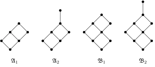
A1 A2 B1 B2

Figure 6: The algebrasA1,A2,B1,B2

Example 52.

1. Every finite distributive lattice is a Heyting algebra. This immediately follows from Proposition 51(2), since every finite distributive lattice is complete and satisfies the infinite distributive law.

2. Every chainCwith a least and greatest element is a Heyting algebra and for everya, b∈Cwe have

a→b=n1 ifa≤b,

b ifa > b.

3. Every Boolean algebra Bis a Heyting algebra, where for everya, b ∈B

we have

a→b=¬a∨b

Exercise 53. Give an example of a non-complete Heyting algebra.

The next proposition characterizes those Heyting algebras that are Boolean algebras. For the proof see, e.g., [20, Lemma 1.11(ii)].

Proposition 54. Let A= (A,∨,∧,→,0) be a Heyting algebra. Then the fol-lowing three conditions are equivalent:

1. Ais a Boolean algebra,

2. a∨ ¬a= 1 for everya∈A, 3. ¬¬a=afor everya∈A.

4.2

The connection of Heyting algebras with Kripke

frames and topologies

R(w) ={v∈W :wRv},

R−1_{(w) ={v∈W :vRw},}

R(U) =S_w∈UR(w),

R−1_{(U) =}S

w∈UR

−1_(w).

A subsetU ⊆W is called an upsetifw ∈U and wRv impliesv ∈ U. Let

U p(F) be the set of all upsets ofF. Then (U p(F),∩,∪,→,∅) forms a Heyting algebra, where U →V ={w ∈W : for everyv ∈ W with wRv ifv ∈U then

w∈V}=W \R−1_(U\V).

Exercise 55. 1. Verify this claim. That is, show that for every Kripke frame

F= (W, R), the algebra (U p(F),∩,∪,→,∅) is a Heyting algebra.

2. Draw a Heyting algebra corresponding to the 2-fork frame (W, R), where

W ={w, v, u} andR={(w, w),(v, v),(u, u),(w, v),(w, u)}.

3. Draw a Heyting algebra corresponding to the frame (W, R), where W = {w, v, u, z} andR={(w, w),(v, v),(u, u),(z, z)(w, v),(w, u),(w, z),(v, z)}. 4. Show that if a frameFis rooted, then the corresponding Heyting algebra

has a second greatest element.

LetF= (W, R) be a Kripke frame. Let Abe a set of upsets of Fclosed under ∩,∪,→and containing ∅. ThenA is a Heyting algebra. A triple (W, R,A) is called ageneral frame.

We will next discuss the connection of Heyting algebras with topology. Definition 56. A pair X = (X,O) is called a topological space if X 6=∅ and

Ois a set of subsets of X such that

• X,∅ ∈ O

• If U, V ∈ O, thenU∩V ∈ O

• If Ui∈ O, for every i∈I, thenSi∈IUi∈ O

For Y ⊆X, the interiorof Y is the setI(Y) = S{U ∈ O : U ⊆ Y}. Let X = (X,O) be a topological space. Then the algebra (O,∪,∩,→,∅) forms a Heyting algebra, whereU →V =I((X\U)∪V) for everyU, V ∈ O.

Exercise 57. Verify this claim. That is, show that for every topological space X = (X,O), the algebra (O,∪,∩,→,∅) is a Heyting algebra.

We already saw how to obtain a Heyting algebra from a Kripke frame. Now we will show how to construct a Kripke frame from a Heyting algebra. The construction of a topological space from a Heyting algebra is more sophisticated. We will not discuss it here. The interested reader is referred to [20,§1.3].

• a, b∈F impliesa∧b∈F

• a∈F anda≤bimplyb∈F

A filterF is calledprimeif

• a∨b∈F impliesa∈F or b∈F

In a Boolean algebra every prime filter is maximal. However, this is not the case for Heyting algebras.

Exercise 58. Give an example of a Heyting algebraAand a filterF ofAsuch thatF is prime, but not maximal.

Now let W :={F : F is a prime filter ofA}. For F, F0 _{∈W we put F RF}0 _if F⊆F0_{. It is clear thatRis a partial order and hence (W, R) is an intuitionistic}

Kripke frame.

Exercise 59. Draw Kripke frames corresponding to: 1. The two and four element Boolean algebras. 2. A finite chain consisting ofnelements forn∈ω. 3. The Heyting algebras drawn in Figure 6.

4. Show that if a Heyting algebraAhas a second greatest element, then the Kripke frame corresponding toAis rooted.

Let A = (A,∧,∨,→,⊥) and A0 _{= (A}0_,∧0_,∨0_,→0_,⊥0_{) be Heyting algebras. A}

maph:A→A0 _{is called aHeyting homomorphismif}

• h(a∧b) =h(a)∧0_h(b)

• h(a∨b) =h(a)∨0_h(b)

• h(a→b) =h(a)→0_h(b)

• h(⊥) =⊥0

An algebra A0

is called a homomorphicimage ofA if there exists a homomor-phism fromAontoA0

. Let A and A0

be two Heyting algebras. We say that an algebra A0

is a

subalgebraofAifA0_{⊆Aand for everya, b∈A}0 _{a∧b, a∨b, a→b,⊥ ∈A}0_.

Aproduct A×A0 _of

AandA0 _{is the algebra (A×A}0_{,∧,∨,→,⊥), where}

• (a, a0_{)∧(b, b}0_{) := (a∧b, a}0_∧0_b0₎

• (a, a0_{)∨(b, b}0_{) := (a∨b, a}0_∨0_b0₎