Article
Dynamic Vehicle Routing Problem with Multiple
Depots
Kwankaew Meesuptaweekoon
aand Paveena Chaovalitwongse
b,*
Department of Industrial Engineering, Faculty of Engineering, Chulalongkorn University, Bangkok 10330, Thailand
E-mail: a[email protected], b[email protected] (Corresponding author)
Abstract. The Vehicle Routing Problems (VRPs) has been extensively studied and applied in many fields. Variations of VRPs have been proposed and appeared in research for many decades. Dynamic Vehicle Routing Problem with Multiple Depots (D-MDVRP) extends the variation of VRPs to dynamism of customers by knowing the information of customers (both locations and due dates) at diverse times. An application of this problem can be found in food delivery services which have many service stores. The customer delivery orders are fulfilled by a group of scattered service stores which can be analogous to depots in D-MDVRP. In this example the information of all customer orders are not known at the same time depending on arrivals of customers. Thus the objective of this operation is to determine vehicle routing from service stores as well as dispatching time. This paper aims to develop a heuristic approach for D-MDVRP. The proposed heuristic method comprises of two phases: route construction and vehicle dispatch. Routes are constructed by applying the Nearest Neighbor Procedure (NNP) to cluster customers and select a proper depot, Sweeping and Reordering Procedures (SRP) to generate initial feasible routes, and Insertion Procedure (IP) to improve routing. Then the determination of dispatch is followed in the next phase. In order to deal with the dynamism, the dispatch time of each vehicle is determined by maximizing the waiting time to provide the opportunity to add more arriving customers in the future. An iterative process between two phases is adopted when a new customer enters the problem, and the vehicles are dispatched when the time becomes critical. From the computational study, the heuristic method performs well on small sized test problems in a shorter CPU time compared to the optimal solutions from CPLEX, and provides an overall average of 8.36 % Gap. For large size test problems, the heuristic method is compared with static problems, and provides an overall average of 3.48 % Gap.
Keywords: Vehicle routing problem, multiple depots, dynamic problem, heuristic, nearest neighbor procedure, sweeping and reordering procedures, insertion procedure.
ENGINEERING JOURNAL Volume 18 Issue 4
1.
Introduction
In Vehicle Routing Problems (VRPs), routes for identical vehicles at the depot are determined, so that each customer is visited exactly once, and the total routing is minimized. After Dantzig and Ramser [1] introduced VRP, various types of this problem have been explored and solution approaches have been proposed. A number of variations of VRP have been extensively studied and applied in many firms [2], namely, the delivery of meal [3-5], the distribution of chemical products, petroleum products, gases and fuels [6-9], the delivery of soft drinks [10], etc. The well-known variations of VRP [11] are the Capacitated Vehicle Routing Problem (CVRP), where vehicles have limited capacities; the Vehicle Routing Problem with Time Windows (VRPTW), where the vehicles have to service or visit customers in the specific time frame; the Vehicle Routing Problem with Pick-up and Delivery (PDP), where the vehicles have to pick-up and deliver goods at given locations; the Heterogeneous Fleet Vehicle Routing Problem (HVRP), where the vehicles are different in dimensions of types and capacities; the Multi-Depot Vehicle Routing Problem (MDVRP), where there are several depots to select for starting or ending of routes; Dial-A-Ride-problem (DARP) which involves moving customers between locations. Wilson and Colvin [12] claimed to be the first reference to a dynamic vehicle routing problem. This paper presents DARP where customers appear dynamically, and the insertion heuristic method is applied to plan trips from an origin to a destination. Psaraftis [13] also introduced the concept of immediate request where the current route has to be changed in order to respond to customers as soon as possible. Later, many works are considered to be dynamic vehicle routing problems (D-VRP) in which new requests arrive dynamically.
Dynamic Vehicle Routing Problem with Multiple Depots (MDVRP) is classified in MDVRP and D-VRP because there are several depots to dispatch vehicles, and the demands of customers dynamically enter the system. All the inputs are unknown and revealed dynamically during routes execution. According to the taxonomy of vehicle routing problems by information evolution and quality, this problem can be called the dynamic and deterministic problems [12]. The evolution of inputs causes the deviation of this problem compared to other MDVRP. In D-VRP, most research introduced problems that design routes before dispatch vehicles and allowed minor changes during the process [14, 15] or consisted of designing routes in an online situation and communicated with the vehicle in order to assign the next customer to visit [16, 17]. The inputs which dynamically arrival can be a demand for goods or services [12]. In this work, demand for goods or services do not know simultaneously and the vehicles have to contain goods for all known demands before leaving the depot. So, the routes cannot be changed during the execution. All customers in the route have to be known before routing. Therefore, it is necessary to carefully consider current customers and current routes before dispatching vehicles because the routes can be changed only when the vehicles are still at the depot. There are real world problems related to D-MDVRP, for example, food or grocery delivery. In these businesses, once customers call the call centre, the call centre takes orders and assigns them to the selected store with assurance to deliver the order in committed time. After receiving the order, the store prepares food or pick up the pre-packaged food for delivery. The customer service level must be evaluated. Consistently prompt delivery is the most important aspect in customer’s view. However, quickest delivery may entail significant costs. Therefore, management of the delivery system to facilitate timely delivery while minimizing the cost of transportation is important [18]. The minimum distance routing provides many benefits. First, it allows more available time for limited resources ready to cater delivery at stores or depots. Secondly, delivery with the optimum route cut down the cost of transportation. Finally, transportation is not the core business of food delivery firms; so maintaining confidence of customer service with low cost is an accomplishment.
This paper aims to introduce the Dynamic Vehicle Routing Problem with Multiple Depots and propose a heuristic approach. As mentioned before, this problem has dynamic demands which arrive in the system at different times. The dynamic demands obviously affect the solution because they change the problem at the instant they arrive at the system. Moreover, the guaranteed time is hard constraint in this problem. In addition, construction of routes from several available depots with minimum distances as the objective is the challenge of this research.
2.
Problem Description
The problem can be explained by using the classic version of MDVRP which is defined on a Graph G = (VC U VD, E). Where VC is a set of customers, VD is a set of depots and E is a set of edges between
customer and customer and customer and depot. A number of capacitated vehicles are m while Q is a maximum capacity of each vehicle. The distance of route, calculated by assuming Euclidian distance, is associated with every edge in routes total to times of service. The travelling rate is 1 unit of distance/1 unit of time.
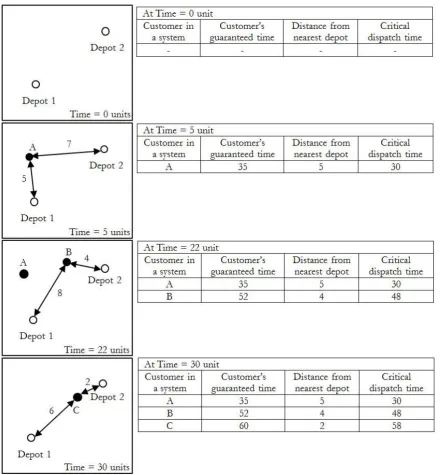
In this problem, the customers are revealed dynamically during the routing process. Each customer has a demand (q) and a guaranteed time (G) which indicates the latest time for servicing. Therefore, in each state of time, there is a different number of customers to consider due to the difference in the arrival time and a guaranteed time which affects the latest time to dispatch the vehicle to visit each customer in the committed time window. Figure 1 shows the dynamically change of the customers of the illustrated problem which has the guaranteed time = 30 units.
[image:3.595.71.513.266.742.2]As shown in Fig. 1, at the beginning, there is no customer in the system. Later, customer A comes in the system at Time = 5 units, then customer B arrives at Time = 22 units. Lastly, customer C arrives at Time = 30 units. The set of customer has changed over time, it has more customers when new customers arrive and has fewer customers when customers have to be visited. At time = 30 units, there are 3 situations which could happen with the set of customers: first, the set is consisted of customers A, B and C and the vehicle has to start to visit customer A at time = 30 units because of the critical dispatching time, second, the set consisted of customers B and C because customer A is already serviced, lastly, the set consisted of only customer C because customer A and customer B are serviced. Related to the classic problem, VC of
this problem has changed over time but VD is revealed at the beginning. These situations provides the
difference between this considered problem and the classic problem.
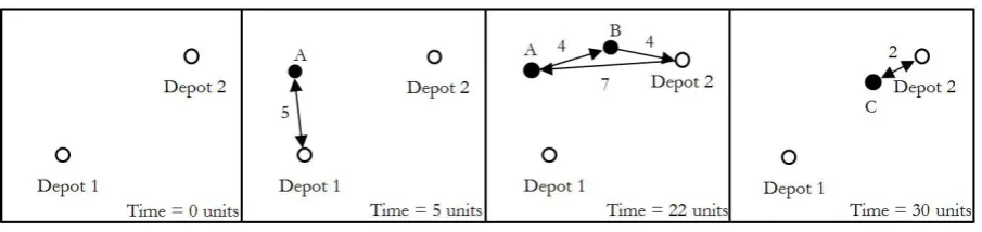
As mentioned earlier, each demand comes in the system at a different time, hence the arrival time is collected once the demand enters the system and the time window is determined immediately. The time window of each customer is the time between the arrival time and the due date (due date = arrival time + guaranteed time). The guaranteed time is a constant and known at the beginning. In this incident, the actual time is instrumental in monitoring the maintenance of the results from the system to satisfy the time constraint. Figure 2represents the graph of the illustrated problem and the solutions which are affected by the dynamism of the customers. The expected results are routes and dispatch time for each route and the objective of this problem is to minimize the total distance while satisfying the following conditions:
1. Every customer is served by exactly one route. 2. Every route starts and ends at the same depot.
3. The overall demands of customers in the same route do not exceed Q. 4. The customer is serviced under the guaranteed time.
Fig. 2. The illustrated problem and the solutions.
As shown in Fig. 2, there are two depots to select. The unit of distance is identical to the unit of time. The critical dispatching time or the latest time of departure of each vehicle is determined after designed the routes. The vehicle is assigned to wait at the depot as long as possible, hence there are at least one customer whose vehicle is visited at a due date. At each state of time, if the new customer arrives at the system, the former solutions are neglected and all routing processes will be applied for all current customers to design new solutions. To simplify this, the solution for dispatching the vehicle can be as follows:
At time = 0: There is no customer arrives to the considered problem. At time = 5: Customer A arrives to the problem and the solution is
Routing: Depot 1 – Customer A – Depot 1 Critical dispatching time: Time = 30
Total distance: 10 Cumulative distance: 10
At time = 22: Customer B arrives to the problem and the solution is Routing: Depot 2 – Customer A – Customer B – Depot 2 Critical dispatching time: Time = 28
Total distance: 15 Cumulative distance: 15
At time = 30: Customer C arrives to the problem and the solution is Routing: Depot 2 – Customer C –Depot 2
Critical dispatching time: Time = 58 Total distance: 4
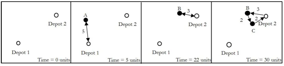
[image:4.595.73.526.364.471.2]From the above solutions, a better solution from Time = 0 units to Time = 30 units could exist if the first route is executed (Depot 1 – Customer A – Depot 1) and Customer B and C are delivered by the same vehicle because the cumulative distance will be 17 as shown in Fig. 3. At this point, the dispatching time decision is important because it is affected by the dynamic arrivals of the customer. Moreover, this paper has considered more constraints, customers and depots comparing with this illustrated problem which make the problem to be more complex to find good solutions.
Fig. 3. The illustrated problem and the new solutions.
3.
Literature Review
In order to deal with D-MDVRP, approaches for MDVRP are explored. Exact algorithms for the MDVRP are rare. According to Renaud et al. [19], only two exact algorithms have been proposed for the MDVRP. The first algorithm was developed by Laporte et al. [20] , which is a branch and bound algorithm. Another algorithm was also proposed by Laporte et al. [21], which is the same algorithm modified to solve asymmetric MDVRPs while the first one was developed for symmetric problems. Even though mathematic model provides optimum solutions but it is inefficient in the evaluation time consumption and it is inappropriate to apply to large problems. Since the VRP is NP-hard, D-MDVRP which poses more restrictions than general VRP also belong to NP-hard problems [22]. Therefore, “Good enough, fast enough” is the interested and realistic characteristic of the approach. The fast solutions can be separated to two different types; heuristics and metaheuristics. The notable vehicle routing problem heuristics can be divided to construction heuristics, e.g., Nearest Neighbor Procedure, Insertion Procedure, Clarke and Wright algorithm and improving heuristics, e.g., 2-Opt method, 3-Opt method, k-Opt method. Metaheuristics are developed after heuristics and also appeared in many researches lately. The acclaimed metaheuristics are Simulated Annealing, Tabu Search, Genetic Algorithm, Neural Nets Algorithm, and Ant Colony Algorithm.
Approaches for MDVRP are explored to develop the proper approach for this problem. Abundant heuristics and metaheuristics were developed for the MDVRP. “Cluster first, route second” method has been applied generally even in real situations. Most businesses cluster customers to the responsible depot by area. As a result, each depot will have to deliver goods to customers separately or MDVRP is transformed to VRP. Crevier et al. [23] proposed the best known solutions for the MDVRP. Their algorithm begins by clustering the customer at the nearest depot, and then a sweep method is applied to each depot. Later, they improved the route by transferring the customer in the same depot or across other depots. Clustering customers at the nearest depot then applying the VRP algorithm and finally improving the solution by the exchange of customer within/between a depot is the method that has been used extensively. However, the initial routes originally routed by basing on the nearest depot affect the domain of better solutions. The desired approach should route and cluster customers based on the routes which change at the moment when the new customer has arrived.
In order to deal with the dynamism, Psaraftis [24] suggested that the dynamic problem should be solved as soon as possible and the algorithm should be flexible and provides a good solution while consuming a short time. Continuous re-optimization is one method adopted by this research. The algorithm solves the problem every time there are changes in inputs. Therefore, good routes can be changed with every customer’s arrival. Due to the problems’ dynamism over time, optimal solutions from CPLEX of overall problems cannot be found. The dynamic approaches have to rely on the heuristic approach in order to quickly compute a solution to the current state of the problem.
[image:5.595.70.527.167.273.2]and short time consumption algorithm is preferable. The “quicker” solution algorithms are natural to adopt for route construction and improvement for dynamic response [25]. Therefore, in order to find good solutions for this specific problem, efficient heuristic approaches which are assigned to find good solution every time the problem changes should be adopted.
4.
Proposed Heuristic Approach
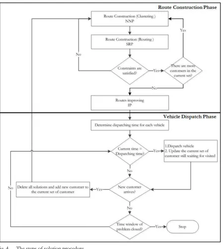
The proposed heuristic approach comprises of two phases: route construction and vehicle dispatch. The route construction phase deals with constructing and improving routes for the current set of customers while the vehicle dispatch phase determines the dispatching time for each vehicle.
In route construction phase, the problem is considered as static problem with the current set of customer. The well-known heuristic approaches which are frequently adopted in static VRP are adapted to solve this problem. Three heuristic methods are adopted and applied for finding solutions to the considered problem: Nearest Neighbor Procedure (NNP), Sweeping and Reordering Procedures (SRP), and Insertion Procedure (IP). Iterative process between NNP and SRP are applied to generate a good feasible route or it can be called “Cluster and route at the same time”. The modified NNP is applied to cluster a customer to a proper depot and then group customers into the same vehicle while before actually adding another customer into the considered group, SRP is applied to arrange order for customers in order to ensure that customers in the same group can be constructed a feasible route. Finally, IP is used to improve the initial routes from NNP and SRP. After the entire process is done, the heuristic approach will provide solutions by selecting the shortest routes to determine the dispatch time in the next phase.
In vehicle dispatch phase, the dispatch time of each vehicle is determined. It can be the longest waiting time that the vehicle can wait (until reaching the critical time of each route) to provide the opportunity to add more future customers to the routes. So, there is at least one customer that the vehicle visits at a critical time or a due date. At this point, the developed decision model provides a longer waiting time for dispatching vehiclescomparing with sending the vehicle to the customer after receiving orders decision (the vehicle does not have to wait the new customers for servicing). Also, it provides a shorter waiting time comparing to holding the customer order as long as possible decision because the feasible routes might be a “one-customer-route” due to a time constraint. To provide update good solutions, the solutions of each state of time are deleted and heuristics reprocess again if there is a new customer entering the system. The details of the mentioned heuristic approach applied to this problem are explained as follows and the steps of solution procedure are drawn in Fig. 4.
4.1. Nearest Neighbor Procedure (NNP)
Nearest Neighbor Procedure (NNP) is the method for clustering customers to the group which all members will be visited by the same vehicle or route. In this heuristic, the nearest customers which are usually determined by a distance between nodes (customer or depot), Euclidian distance, are grouped together, and then the next nearest customer to the first couple is added. This procedure is continued until there is no nearest unvisited customer exits. To close the route, the vehicle returns to the starting depot [26, 27]. For the multiple depots problem, customers can be visited by a vehicle from any depot that is nearest to customers.
In the ordinary NNP, Euclidian distance is used as the only criterion to select the nearest visiting node. However, the Euclidian distance indicates only a distance between nodes which does not provide a relationship of nodes in the group. For simplicity, the relationship between two nodes can be explained by distances and directions. Determining both distances and directions might add more complexity to construct routes. To solve this weakness, square grids counting is applied instead of Euclidian distance. It determines a relationship between more than two nodes in the group and it is straightforward to compute and used as a criterion.
axis-aligned directions is applied. Figure 5 illustrates the difference between Manhattan distance and the Euclidean distance and Fig. 6 shows the Manhattan distance applied on the map to calculate grids.
[image:7.595.75.525.117.619.2]Fig. 4. The steps of solution procedure.
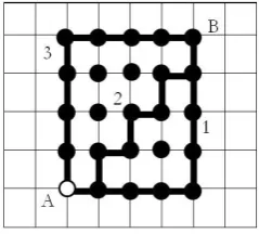
[image:7.595.209.388.649.725.2]In Fig. 6, the Manhattan distance from A to B is 8 units, whether by calculating from distances 1, 2, or 3. In this paper, grids under all possible Manhattan routes are called grid area. The heuristic method will calculate the grid area between the location of each depot and customer who enters system. Then, a customer in a location that generates the minimum grid area between its location and a depot will be clustered together and listed as the first group to consider adding more customers. The next customer is added to an existing group if their locations provide the minimum grids for the group. As shown in Fig. 7, the counting grids of nodes A, B and C equals 18 grids. The relationship can be determined by counting intersect grids of all customer locations in the group. If the group generates the minimum grid (Primary criteria) area and minimum intersect grids (Secondary criteria), the group is considered to be applied in SRP first. Again in Fig. 7, the intersect grids of nodes A, B and C are equal to 9 grids.
Fig. 6. The Manhattan distance and square grids area.
Fig. 7. The grid area of node A, B and C.
To ensure that the preferable nodes or customers can be added to the considered group, overall capacities are determined to meet the constraint of capacity. Each customer can be added to the considered group if the SRP can find the feasible route for the group. NNP and SRP are iteratively processed until no more customers in the system and will start over if the new customer arrives. By counting square grids, distances and directions are simultaneously considered in clustering customers. The ability to quickly compute directions and distances from one arbitrary node to another and the flexibility to generate solutions for the dynamic problem are the reasons that this developed method is applied in this work.
4.2. Sweeping and Reordering Procedure (SRP)
As described in the previous procedure, the customers are grouped together by using minimum grid area and intersect grids as the criterion. In this procedure, SRP is utilized to ensure that feasible routes to serve those customers are available.
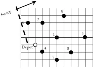
[image:8.595.238.358.210.318.2] [image:8.595.72.511.352.459.2]Fig. 8. A sweep method.
4.3. Insertion Procedure (IP)
After NNP and SRP have been performed, solutions can be improved to minimize the total distance by an IP [26]. Each node in initial routes will be analyzed to determine placement of orders in routes. Customers’ order or routes will be changed if the total distance is decreased, and the routes are still feasible. To finish the solutions, interchange of customers over depots is in consideration. The customer will be inserted into other routes should it is deemed necessary. This iterative process needs to exceed or at least equate the former results, and must turn feasible solutions. Figure 9 demonstrates an example of before and after solutions resulted by an insertion procedure.
Fig. 9. An insertion procedure.
Because the complexity of this problem is NP-hard, the first best cluster of a customer and a selected depot may not provide the best or optimal solutions. Hence, in the beginning of NNP, the heuristic method will generate the list of the first clusters by sorting solutions from the best to the worst. Each cluster in the list is examined to find out the final routes from IP for comparison of the total distance when the last cluster in the list is completed. Finally, the minimum distance solution will be selected for creation of dispatch event.
5.
Computational Experiments
[image:9.595.198.362.100.221.2] [image:9.595.124.466.380.507.2]5.1. Test problems
In relation to the well-known research by Solomon [29], there are several factors that mainly affect the distances and characters of routes: geographical data, the number of customers serviced by a vehicle, the percentage of time-constrained customers, and the tightness and dislocation of the time windows. In this work, locations of customers are randomly generated and the main parameters are the ratio of an inter-arrival time to a guaranteed time which are related to the percentage of time-constrained customers; tightness and disposition of the time windows; average of customers per vehicle or number of customers serviced by a vehicle; size of problems and a location of each depot in the multiple depots problems.
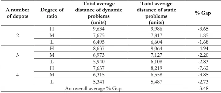
[image:10.595.68.517.375.434.2]In dynamic problems, customers can be served by the same vehicle if their time windows are overlapped in feasible routes’ construction. A time window of each customer in this problem is the time between an arrival time and a due date which depends on a guaranteed time for servicing. Hence, the arrival time and the guaranteed time are important for identifying the characteristic of dynamic problems and they affect the number of customers to construct routes as well. To clarify this, in problems that have a short inter-arrival time and a long guaranteed time, there are many arriving customer in the system available to construct routes for servicing and if an inter-arrival time are decreased to zero, the problems are likely to be static problems (all customers are known at the beginning). In contrast, in a long inter-arrival time and the guaranteed time is the same as the previous example, there are few or just one customer to consider for routing in each state of time because the customers have to be visited before the next customer arrives at the system. Therefore, in this work, a ratio of mean inter-arrival time to a guaranteed time is considered to formulate the test problems. Parameters defined a ratio of an inter-arrival time to a guaranteed time are shown in Table 1.
Table 1. Parameters defined a ratio of an inter-arrival time to a guaranteed time.
Parameters Ratio of mean of inter-arrival
time to guaranteed time Degree of ratio Mean of inter-arrival time Guaranteed time
40 200 1:5 High (H)
20 200 1:10 Moderate (M)
10 200 1:20 Low (L)
The inter-arrival time is assumed to be exponentially distributed with a mean µ for each customer but the guaranteed time is a constant and fixed at 200 units of time. Therefore, there are different numbers of customers to consider dependent on the degree of ratios. The number of customers indicates the size of problem or decision variables as well. To clarify this, if the degree of ratio is low, the problems are likely to have more customers for route construction than high ratio problems, because there are more chance to accumulate the number of customers at any state of time or the number of customers at any point of time depends on the degree of ratio.
Vehicle capacity and an average demand capacity are parameters for identification of average of customers per vehicle. In this work, average demand capacities vary between 15-20 units with uniform distribution and vehicle capacity is fixed at 10,000 units in order to render vehicle capacity constraint invalid for simplicity of discussion about dynamic characteristic of the problem.
A number of depot and an average customer per depot are important characteristics in multiple depots problem. In these experiments, the number of depot is set to 2 and 4 and depot locations within the relevant area (100 unit2) are fixed as illustrated in Table 2. The fixed locations as shown in Fig. 10 are
designed for equally separating the area to service customers and providing unbiased solutions because the locations of customers are randomly generated.
Table 2. A number of depot and location.
A number of depots Depot 1 Depot 2 Depots location Depot 3 Depot 4
2 (25,25) (75,75)
3 (25,25) (75,25) (50,75)
[image:10.595.120.460.670.726.2]Fig. 10. The location of depots.
5.2. The Experiment of Small Size Problems
[image:11.595.105.489.79.204.2]In this experiment, the heuristic solutions are compared with the optimal CPLEX solutions. Test problems for CPLEX are identified as static problems because all parameters and inputs are known in advance in order to find the optimal solutions. According to the limitation of CPLEX, there are 12 customers assigned to a test problem in order to achieve solutions in a reasonable time. There are 10 sets of customer locations which are divided into 9 characteristics of problems (high, moderate, low ratio and 2, 3, 4 depots). Therefore, 90 problems are tested. Table 3 illustrates the percentage gap between the total distances of solutions from the heuristic and CPLEX.
Table 3. The results from experiments of small size problems (comparing the performance between the heuristic and CPLEX).
A number
of depots Degree of ratio % Gap
Heuristic CPU time (sec) CPLEX CPU time (sec) Avg. Min. Max. Avg. Min. Max.
2
H 8.03 0.081 0.072 0.089 2,056.71 107 5,331
M 15.02 0.177 0.091 0.203 1,464.71 205 3,133
L 13.76 0.155 0.120 0.176 1,222.86 49 2,123
3
H 6.69 0.086 0.072 0.098 1,774.86 252 5,453
M 6.61 0.089 0.078 0.096 1,508.57 327 2,760
L 11.14 0.090 0.082 0.112 633.29 131 1,408
4
H 1.92 0.075 0.064 0.087 603.29 58 1,391
M 4.24 0.079 0.068 0.094 1,260.14 32 2,469
L 7.79 0.072 0.059 0.079 519.57 72 1,451
An overall average
% Gap 8.36
As shown in Table 3, the first and second column indicate the problem characteristics while the third shows the percentage gap between the total distances of solutions from the heuristic method and CPLEX (% Gap). The fourth column shows the computational time of the heuristic method while the seventh column shows the computational time of CPLEX and the eighth and ninth column show the minimum and maximum time to find the optimal solution of CPLEX respectively. The result shows that the heuristic method can find good solutions with an average of 8.36% Gap, 1.92% Gap at minimum, and 15.02% Gap at maximum from the optimal solutions which are solved when the problems are static. The heuristic method consumes much less computational time comparing with CPLEX. Moreover, CPLEX has a variation of time consuming as shown in the last two columns while the heuristic method has more consistency at this point.
According to the 3rd column, an average of % Gap separated by the degree of ratio indicate that the
[image:11.595.81.518.373.516.2]Table 4. The results from experiments of small size problems (comparing the performance of the heuristic on static and dynamic problems).
A number
of depots Degree of ratio
Total average distance of dynamic
problems (units)
Total average distance of static
problems (units)
% Gap
2
H 595.63 611.08 -2.68
M 511.40 537.91 -5.74
L 478.78 498.96 -6.06
3
H 479.31 479.48 0.06
M 419.04 432.71 -3.67
L 397.50 415.31 -5.33
4
H 394.52 400.12 -1.38
M 368.87 370.33 -0.54
L 349.15 355.95 -2.34
An overall average % Gap -3.08
The result in Table 4 presents the problem characteristics in the first and second columns. The third and fourth columns show the average of total distance from solving dynamic and static problems and the percentage gap (% Gap) between total average distances of solutions obtained from testing the heuristic on dynamic and static problems in the fifth column. The result states that the developed heuristic performs well on dynamic test problems in comparison to static problems as proven by the negative value of % Gap.
5.3. The Experiment of Large Size Problems
To date, there is no referential benchmark for dynamic vehicle routing problem [12]. Many authors based their computational experiment on adaptations of the Solomon instances [25, 29-32]. Therefore, comparison of the results between dynamic and static problem is an interesting experiment for evaluation of the heuristic and it is reasonable to apply in the experiment of large sized problems.
Dynamic problems tested in this experiment are 10 sets of 200 customer locations which are divided into 9 characteristics of problems (high, moderate, low ratio and 2, 3, 4 depots). Hence, 90 problems are tested the same as the former experiments. Static problems are identical to the dynamic problem but an inter-arrival time becomes zero for every customer. In this case, at the beginning, there are 200 customers suitable for construction of routes for static problems. The percentage gap between the total distances of solutions obtained from testing the heuristic method on dynamic and static problems are shown in Table 5.
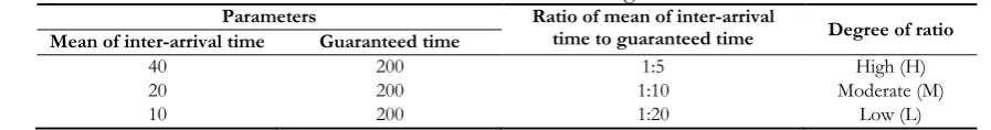
Table 5. The results from experiments of large size problems.
A number of depots
Degree of ratio
Total average distance of dynamic
problems (units)
Total average distance of static
problems (units)
% Gap
2
H 9,634 9,986 -3.65
M 7,675 7,817 -1.85
L 6,495 6,604 -1.68
3
H 8,637 9,064 -4.94
M 6,973 7,127 -2.20
L 5,940 6,108 -2.83
4
H 7,637 8,219 -7.62
M 6,315 6,558 -3.85
L 5,341 5,487 -2.73
An overall average % Gap -3.48
The result in Table 5 presents the problem characteristics in the first and second columns. The third and fourth columns show the average of total distance from solving dynamic and static problems and the percentage gap (% Gap) between total average distances of solutions obtained from testing the heuristic on dynamic and static problems in the fifth column. The result states that the heuristic method performs well on dynamic test problems in comparison to static problems as proven by the negative value of % Gap.
[image:12.595.118.476.514.665.2]obtained from static problems offer short distances and require many vehicles for dispatch events. These situations provide short routes in every state of time but long total visiting distances. It demonstrates that this heuristic method should consider only customers in the same time frame to construct a good route. Time frame is also beneficial in clustering proper groups in problems with many customers in consideration and few depots for selection.
In summary, the developed heuristic method can be applied to problem of interest. The heuristic performs well in all given characteristics by consumption of very short computational time. It is able to generate good solutions when the problems are changed dynamically. The results indicate that the heuristic provides good solutions in comparison to optimal solutions of static problems provided by CPLEX in the experiment of small size problems. In addition, the heuristic is more suitable to find solutions from dynamic problems than static problems as shown in the experiment of large sized problems.
6.
Conclusion
This paper has D-MDVRP in consideration. This problem’s characters are more specific in comparison to the general MDVRP. The dynamism of customers changed the problems over time. The proper heuristic was required to find good solutions for this specific problem. NNP utilizing grid as a criterion provided the method to cluster customers and minimize routing distance while simultaneously assigning a customer group to proper depot. SRP were applied to routing and searching good routes. IP improved routing by minimizing the distances. The heuristic method was tested on generated problems to evaluate its efficiency and identify characteristics of considered problems under which the heuristic method performs well. Moreover, results provide knowledge and urge improvement of heuristic approaches for this problem of interest in future research.
As discussed in the results part, the developed heuristic method provides good solutions in all problem characteristics by the consumption of very short time. Also, the heuristic method performs better if the test problems belong to high ratio of an inter-arrival time to a guaranteed time characteristic and have more depots available for selection. Lastly, the dynamic of problems provides proper groups of customers for consideration in respect of time frame in order to construct good routes.
From the experiment, the solutions can be improved if some customers in the former routes (already dispatched) are clustered in the current routes (awaiting dispatch). However, this proposed heuristic method is developed to construct routes with only one objective, minimization of distances in each state of time. In order to improve routes in dynamic problems, determination of time frame and waiting time of each customer for the purpose of minimization of total distances is interesting for the future study. In addition, this work does not apply the developed heuristic method in real applications, so another subject of future work is to apply the heuristic method in real world problems.
Acknowledgements
The portion of this work was presented at 17th International Conference of the International Journal of
Industrial Engineering – Theory, Applications, and Practice (IJIE). We express gratitude to Prof. Wanpracha Art Chaovalitwongse, Department of Industrial and System Engineering of the University of Washington, for guidance and feedback on the earlier drafts of this paper and recognition to anonymous reviewers for insightful comments.
The authors would like to acknowledge Graduate School, Faculty of Engineering and Resource and Operation Management Research Unit (ROM), Chulalongkorn University, for the financial support to this work.
References
[1] G. B. Dantzig and J. H. Ramser, “The truck dispatching problem,” Management Science, vol. 6, pp. 80– 91, 1959.
[3] O. Braysy, P. Nakari, W. Dullaert, and P. Neittaanmaki, “An optimization approach for communal home meal delivery service: A case study,” Journal of Computational and Applied Mathematics, vol. 232, pp. 46–53, 2009.
[4] P. J. Cassidy and H. S. Bennett, “TRAMP—A multi-depot vehicle scheduling system,” Operational Research Quarterly (1970-1977), vol. 23, pp. 151–163, 1972.
[5] H. Yildiz, M. P. Johnson, and S. Roehrig, “Planning for meals-on-wheels: Algorithms and application,”
Journal of the Operational Research Society, vol. 64, pp. 1540–1550, 2014.
[6] M. Vidovic, D. Popovic, and B. Ratkovic, “Mixed integer and heuristics model for the inventory routing problem in fuel delivery,” International Journal of Production Economics, vol. 147, Part C, pp. 593– 604, 2014.
[7] W. J. Bell, L. M. Dalberto, M. L. Fisher, A. J. Greenfield, R. Jaikumar, P. Kedia, R. G. Mack, and P. J. Prutzman, “Improving the distribution of industrial gases with an on-line computerized routing and scheduling optimizer,” Interfaces, vol. 13, pp. 4–23, 1983.
[8] G. G. Brown, C. J. Ellis, G. W. Graves, and D. Ronen, “Real-time, wide area dispatch of mobil tank trucks,” Interfaces, vol. 17, pp. 107–120, 1987.
[9] M. O. Ball, B. L. Golden, A. A. Assad, and L. D. Bodin, “Planning for truck fleet size in the presence of a common-carrier option,” Decision Sciences,vol. 14, pp. 103–120, 1983.
[10] B. L. Golden and E. A. Wasil, “Computerized vehicle routing in the soft drink industry,” Operations Research, vol. 35, pp. 6–17, 1987.
[11] B. Eksioglu, A. V. Vural, and A. Reisman, “The vehicle routing problem: A taxonomic review,”
Computers & Industrial Engineering,vol. 57, pp. 1472–1483, 2009.
[12] V. Pillac, M. Gendreau, C. Gueret, and A. L. Medaglia, “A review of dynamic vehicle routing problems,” European Journal of Operational Research,vol. 225, pp. 1–11, 2012.
[13] H. N. Psaraftis, “A dynamic programming solution to the single vehicle many-to-many immediate request dial-a-ride problem,” Transportation Science,vol. 14, pp. 130–154, 1980.
[14] D. J. Bertsimas and D. Simchi-Levi, “A new generation of vehicle routing research: Robust algorithms, addressing uncertainty,” Operations Research,vol. 44, pp. 286-304, 1996.
[15] A. Attanasio, J.-F. Cordeau, G. Ghiani, and G. Laporte, “Parallel tabu search heuristics for the dynamic multi-vehicle dial-a-ride problem,” Parallel Computing,vol. 30, pp. 377–387, 2004.
[16] C. Novoa and R. Storer, “An approximate dynamic programming approach for the vehicle routing problem with stochastic demands,” European Journal of Operational Research,vol. 196, pp. 509–515, 2009. [17] N. Secomandi and F. Margot, “Reoptimization approaches for the vehicle-routing problem with
stochastic demands,” Operations Research, vol. 57, pp. 214–230, 2009.
[18] G. Laporte, “What you should know about the vehicle routing problem,” Naval Research Logistics (NRL),vol. 54, pp. 811–819, 2007.
[19] J. Renaud, G. Laporte, and F. F. Boctor, "A tabu search heuristic for the multi-depot vehicle routing problem," Computers & Operations Research,vol. 23, pp. 229–235, 1996.
[20] G. Laporte, Y. Nobert, and M. Desrochers, “Optimal routing under capacity and distance restrictions,”
Operations Research,vol. 33, pp. 1050–1073, 1985.
[21] G. Laporte, Y. Nobert, and S. Taillefer, “Solving a family of multi-depot vehicle routing and location-routing problems,” Transportation Science,vol. 22, pp. 161–172, 1988.
[22] M. Polacek, R. F. Hartl, K. Doerner, and M. Reimann, “A variable neighborhood search for the multi depot vehicle routing problem with time windows,” Journal of Heuristics,vol. 10, pp. 613–627, 2004. [23] B. Crevier, J.-F. o. Cordeau, and G. Laporte, “The multi-depot vehicle routing problem with
inter-depot routes,” European Journal of Operational Research,vol. 176, pp. 756–773, 2007.
[24] H. Psaraftis, “Dynamic vehicle routing: Status and prospects,” Annals of Operations Research,vol. 61, pp. 143–164, 1995.
[25] Z.-L. Chen and H. Xu, “Dynamic column generation for dynamic vehicle routing with time windows,”
Transportation Science,vol. 40, pp. 74–88, 2006.
[26] Y. Marinakis and A. Migdalas, “Heuristic solutions of vehicle routing problems in supply chain management,” in Combinatorial and Global Optimization. 2002, pp. 205–236.
[27] S. S. Ravi, S. Shukla, D. Rosenkrantz, R. Stearns, and P. Lewis, II, “An analysis of several heuristics for the traveling salesman problem,” in Fundamental Problems in Computing,. Netherlands: Springer, 2009, pp. 45–69.
[29] M. M. Solomon, “Algorithms for the vehicle routing and scheduling problems with time window constraints,” Operations Research,vol. 35, pp. 254–265, 1987.
[30] R. W. Bent and P. Van Hentenryck, “Scenario-based planning for partially dynamic vehicle routing with stochastic customers,” Operations Research,vol. 52, pp. 977–987, 2004.
[31] H.-K. Chen, C.-F. Hsueh, and M.-S. Chang, “The real-time time-dependent vehicle routing problem,”
Transportation Research Part E: Logistics and Transportation Review,vol. 42, pp. 383–408, 2006.