Article:
Maher, M.J., Stewart, K. and Rosa, A. (2005) Stochastic social optimum traffic assignment.
Transportation Research B, 39B (8). pp. 756-767. ISSN 0191-2615
https://doi.org/10.1016/j.trb.2004.10.001
[email protected] https://eprints.whiterose.ac.uk/ Reuse
See Attached
Takedown
If you consider content in White Rose Research Online to be in breach of UK law, please notify us by
White Rose Research Online
http://eprints.whiterose.ac.uk/
Institute of Transport Studies
University of Leeds
This is an uncorrected proof version of a paper published in Transportation
Research B. It has been uploaded with the permission of the publisher. It has
been refereed but does not include the publisher’s final corrections.
White Rose Repository URL for this paper:
http://eprints.whiterose.ac.uk/
2460/
Published paper
Maher M.J., Stewart K. and A. Rosa (2005) Stochastic social optimum traffic
assignment. Transportation Research 39B(8), 753-767.
UNC
ORREC
TED
PROOF
2
Stochastic social optimum traffic assignment
3
Mike Maher
*, Kathryn Stewart, Andrea Rosa
4 School of the Built Environment, Transport Research Institute, Napier University, 10 Colinton Road,
5 Edinburgh EH10 5DT, Scotland
Received 8 January 2004; received in revised form 23 February 2004; accepted 26 October 2004
8 Abstract
9 This paper formulates a Stochastic Social Optimum (SSO) that relates to the Stochastic User
Equilib-10 rium (SUE) in the same way as the Social Optimum (SO) relates to the User Equilibrium (UE) in a
deter-11 ministic environment. At the SSO solution, the total of the usersÕ perceived costs is minimised. The
12 formulation and analysis is carried out in a general utility-maximising framework, with the probit and logit
13 models being special cases. Conditions for the SSO flow pattern are derived, from which it can be seen that
14 the marginal social costs play the same role in the SSO as the standard costs play in SUE. In particular, it is
15 shown that the SSO solution can be obtained through the use of an algorithm for SUE, but with the
mar-16 ginal costs replacing the standard costs in the stochastic loading and that optimal tolls are the differences
17 between the marginal social costs and the standard costs. For the case of the logit model an explicit
path-18 based objective function is obtained which is of a pleasing symmetrical form when compared with the
19 objective functions for SUE, SO and UE. Additionally, a link-based objective function for the general
util-20 ity-maximising case is formulated for SSO, which is similar in form to the SUE objective function of Sheffi
21 and Powell.
22 2004 Published by Elsevier Ltd.
23 Keywords:Traffic assignment; Stochastic user equilibrium; Probit model; Logit model; Optimal tolls; Marginal social
24 costs 25
0191-2615/$ - see front matter 2004 Published by Elsevier Ltd.
doi:10.1016/j.trb.2004.10.001
*Corresponding author. Tel.: +44 131 455 2233; fax: +44 131 455 2239.
E-mail address:[email protected](M. Maher).
UNCORRECTED
PROOF
26 1. Introduction
27 In deterministic traffic assignment, there are two different solutions: the User Equilibrium (UE) 28 and the Social (or System) Optimum (SO), corresponding to WardropÕs first and second equilib-29 rium principles (Wardrop, 1952). The UE flow pattern is how we believe things will be, with driv-30 ers choosing their routes selfishly, whilst the SO flow pattern is how the traffic engineer mightlike 31 things to be, in that the total network travel cost is minimised under SO. It is well-known that the 32 SO solution can be found by using the marginal social cost-flow functionsm(x) in place of the unit 33 link cost-flow functionst(x) in an algorithm to produce the UE solution. It is also known that we 34 can make the congestion-minimising SO flow pattern into a UE solution by imposing the toll 35 (ma(xa*)ta(xa*)) on link a, wherex* is the SO solution.
36 Here, we aim to formulate the same principles but in a stochastic environment. The Stochastic 37 User Equilibrium (SUE) solution corresponds to the UE solution with drivers choosing the route 38 which minimises their personal perceived travel cost, and so we seek to define a Stochastic Social 39 Optimum (SSO) which relates to the SUE solution in the same way as the SO solution relates to 40 the UE solution. The SSO solution therefore is that flow pattern which minimises the total of the 41 travel costs perceived by drivers. Just as the SO solution generally requires some drivers travelling 42 on paths which are not the minimum cost paths for that OD pair, so the SSO solution generally 43 requires some drivers to be assigned to paths that are not their minimum perceived cost path. As 44 will be seen later,Yang (1999)has characterised the SSO solution as that which maximises con-45 sumer surplus.
46 We also investigate whether there are similar results for (i) finding the SSO solution by use of an 47 algorithm to produce the SUE solution, and (ii) whether there is a corresponding result about the 48 tolls required to make the SSO solution into a SUE solution.
49 2. Notation and assumptions
50 For convenience, we set out here the notation for the principal variables and parameters used in 51 the analysis to follow in the rest of the paper. This notation largely follows that ofSheffi (1985).
52 xa flow on linka
53 ta ta(xa) = cost of travel along link a, a function of xa only
54 qrs demand between OD pairrs
55 hrsk flow on pathkbetween OD pair rs
56 crsk mean perceived travel cost on pathk between OD pairrs 57 ma ma(xa) = marginal social travel cost on link a¼taþxaddxata 58 drsak 1 if link ais on pathk between OD pairrs, and 0 otherwise 59 Srs expected minimum perceived travel cost between OD pair rs
60 sa value of the toll charged on linka
61
62 In addition to the separability of the link performance functionta(xa), it is assumed throughout
63 the paper that this function is positive, strictly increasing, and convex. Under these conditions, as
con-UNC
ORREC
TED
PROOF
65 tinuous and therefore infinitely divisible, so that in calculating expected perceived travel costs, a 66 limiting Weak Law of Large Numbers applies.
67 3. Defining the SSO
68 In stochastic assignment different drivers have different perceptions of the costs on the links and 69 paths, and we use a distribution of perceived costs to describe these differences. Whereas the SO 70 flow pattern is that which minimises the total network travel cost, the SSO is defined as that flow 71 pattern that minimises the total of the perceived travel costs in the network.
72 To illustrate the concepts, let us first consider the case of a two-path network between a single 73 O–D pair with a fixed demandq. The flows on the paths are denoted byh1andh2(h1+h2=q), a 74 driverÕs perceived values of the path costs are denoted by u1 and u2 and the probability density 75 function of the driversÕperceived costs isf(u1,u2). Firstly, given path flows ofh1 and h2we need 76 to allocate the drivers to the paths so as to minimise the total perceived cost. Generally, this will 77 require some drivers to be assigned to paths that are not their minimum perceived cost paths. See
78 Fig. 1: drivers whose perceived costs lie within the regionR1(above the line BC) will be assigned 79 to path 1; those whose perceived costs lie below BC will be assigned to path 2. The boundary be-80 tween R1and R2is the line BC with equationu2=u1+d2where the value of d2 is such that the 81 probability mass contained within R1 isp1=h1/q. Note that those drivers whose perceived costs 82 fall between the lines BC and OA (theu1=u2line) are those who, for the benefit of the population 83 as a whole, are assigned to their non-minimum cost path.
84 Therefore,d2must be found such that
Z
R1
fðu1,u2Þdu1du2 ¼p1 ¼ h1
q ð1Þ
u1 u2
R1
O
A
B
C
R2
[image:5.544.59.387.375.646.2]d2
UNCORRECTED
PROOF
88 With this assignment, the total expected perceived cost is
zðh1,h2Þ ¼q
Z
R1
u1fðu1,u2Þdu1du2þ
Z
R2
u2fðu1,u2Þdu1du2
ð2Þ
92 Note that the value ofd2 and hence the regionsR1and R2 depend on the path flowsh1,h2 Also, 93 the mean perceived path costsc1andc2are also functions of the path flows, through the cost-flow 94 relations. However, we make the assumption throughout this paper that it isonlythe meansc1,c2 95 that are affected by the path flows; the variances and covariances remain fixed. Therefore, the fol-96 lowing condition holds for the bivariate density function of perceived path costs
fðu1þd1,u2þd2;c1,c2Þ ¼fðu1,u2;c1d1,c2d2Þ 8d1,d2 ð3Þ
100 The choice model is assumed to be a utility-maximising model, including both the logit and probit 101 models. In the logit model, the perception errors are independent Gumbel variates, with fixed 102 variances. In the probit model, the perception errors are multivariate Normal and we assume 103 the (co)variances to be constant (possibly at values related to the free-flow mean costs, as sug-104 gested by Sheffi (1985)[p. 313] in connection with the Sheffi and Powell objective function for 105 SUE).
106 Hence, from (2) and (3), the total perceived network cost, for flow patternhis
zðh1,h2Þ ¼q
Z
u1<u2d2
u1fðu1,u2;c1,c2Þdu1du2þ
Z
u1>u2d2
u2fðu1,u2;c1,c2Þdu1du2
¼q
Z
u1<u2
u1fðu1,u2;c1,c2d2Þdu1du2þ
Z
u1>u2
ðu2þd2Þfðu1,u2;c1,c2d2Þdu1du2
¼q
Z
u1<u2
u1fðu1,u2;c1,c2d2Þdu1du2þ
Z
u1>u2
u2fðu1,u2;c1,c2d2Þdu1du2
þq d2
Z
u1>u2
fðu1,u2;c1,c2d2Þdu1du2
109 Hence
zðh1,h2Þ ¼q Sð ðc1,c2d2Þ þd2p2Þ ¼qSðc1,c2d2Þ þh2d2 ð4Þ
113 whereSdenotes the ‘‘satisfaction’’ or composite travel cost, given for the logit case by the familiar 114 ‘‘logsum’’ formula
Sðc1,c2Þ ¼ 1
h logðexpðhc1Þ þexpðhc2ÞÞ
UNC
ORREC
TED
PROOF
122 3.1. A numerical example
123 To illustrate these ideas, consider a simple example with two parallel paths between a single O– 124 D pair. We assume that the perceived path costs are independent and Gumbel distributed, with 125 meansc1 andc2 and a value of the sensitivity parameterh of 0.1. The two paths have BPR-style 126 cost-flow functions so that the mean path costs are given by, c1= 10 + 0.02h1 and 127 c2= 15 + 0.005h2 The demandq= 1000.
128 Sinceu1 and u2 are Gumbel distributed with meansc1 andc2the proportion p1 of drivers for 129 whom u1<u2d2 is the same as the proportion for whomu1<u2 when the means are c1 and 130 c2d2; that is
p1¼
expðhc1Þ
expðhc1Þ þexpðhðc2d2ÞÞ
133 so that the value of d2 required to give the correct probability massp1=h1/qis
d2¼ 1 h log
h1 h2
c1þc2
136 Hence the SSO objective function in this two-path logit case is
zðh1,h2Þ ¼ q
h logðexpðhc1ðh1ÞÞ þexpðhðc2ðh2Þ d2ÞÞ
1
hlog
h1 h2
c1ðh1Þ þc2ðh2Þ
h2
139 For this example, we can plot the value of this SSO objective function againsth1. For comparison, 140 we also show inFig. 2the plots of the UE, SO and SUE objective functions againsth1. The
posi-0 5000 10000 15000 20000 25000 30000
0 100 200 300 400 500 600 700 800 900 1000
SO
SSO UE
SUE
h1
[image:7.544.105.433.441.643.2]z
UNCORRECTED
PROOF
141 tions of the minima show that the solution for UE ish= (400, 600), that for SO ish= (300, 700), 142 that for SUE ish= (462, 538) and that for SSO ish= (390, 610) (We note in passing that it can be
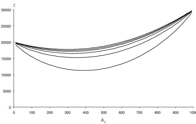
143 verified that, in this case, this SSO solution is the same as the SUE solution that is obtained by 144 replacing the unit cost-flow functions by the marginal social cost-flow functions.). In Fig. 3, we 145 plot the SSO objective function for several values of the sensitivity parameter h 146 (=0.1, 0.25, 0.5, 1 and 2) and it can be seen that ashincreases, the plot of the SSO objective func-147 tion steadily approaches that of the SO objective function, as would be expected, since the degree 148 of variation in the perceived costs is steadily reducing towards zero.
149 We now aim to extend the formulation in(4)to a more general case, with many (generally over-150 lapping) paths between an O–D pair and, subsequently, to multiple O–D pairs. Now, whereas in 151 the SUE case, the user chooses the path for which the perceived cost is minimum, for the SSO case 152 we extend the decision rule for the two-path case to one that states that a driver should be as-153 signed to path j if its ‘‘augmented cost’’ ujdj is smaller than the augmented costs ukdk for
154 all other pathsk. The values of thedjmust then be set such that the proportion assigned by this
155 process to pathjishj/q. To justify this form of decision rule, we consider in the next section a
dis-156 crete version of the problem, before returning to the continuous case thereafter.
157 4. A discrete version of the problem
158 We consider here a discrete version of the problem: that is, we assume that there is a (large) 159 number N of users each of which has the same J paths to choose from. The users have ran-160 domly-drawn and independent sets of values of the perceived path costs uij which we take to
161 be set out in anN·Jmatrix. These costs can be thought of being made up a mean valueljwhich
162 depends on the flow(s) on that path and a perception erroreijthat is drawn from some distribution
0 5000 10000 15000 20000 25000 30000
0 100 200 300 400 500 600 700 800 900 1000
h1
[image:8.544.108.437.92.301.2]z
UNC
ORREC
TED
PROOF
163 (Gumbel or Normal) with zero mean and constant variances (so that as the mean of any path 164 changes through congestion effects so the perceived costs for all users on that path change by 165 the same amount).
166 The problem is how to assign users to paths so as to minimise the total perceived cost, whilst 167 ensuring that the numbers assigned to each path are as given. That is, given that we are to assign a 168 total ofnj(j= 1,. . .,J) users to pathj(n1+n2+ +nJ=N), we are to find the optimal values of
169 the variablesyij(whereyij= 1 if useriis to be assigned to pathj, and zero otherwise) so as to
min-170 imise the total perceived costz¼P
ijyijuij. As each user is to be assigned to just one path we must
171 haveP
jyij¼1 and since we must satisfy the constraint on the numbers assigned to each path, we
172 must have P
iyij ¼nj. This is a special case of the ‘‘classical transportation problem’’ (special in
173 that the row totals are all 1).
174 It is well-known (see, for example,Taha, 1976) that, for such a problem, a basic solution con-175 sists of exactly (N+J1) of theNJcells being used. Of these it is clear that exactlyNwill take 176 the value 1 (one per row). The otherJ1 must be zeroes (but still be basic). These zero-valued 177 basic cells must therefore appear in at most (J1) rows (they could all be in a single row, or at 178 the other extreme could each be in a different row). The optimal solution is a basic solution and 179 the standard solution algorithm iterates through a sequence of basic solutions until the optimum 180 is reached, with the value of the objective functionz reducing at each iteration.
181 It is known that the following conditions hold for any basic solution at any iteration. For each 182 basic cell (whether its yijvalue is 0 or 1)
uij¼aiþbj
185 and for each non-basic cell a negative value of
vij¼uijaibj
188 indicates that if this cell were to be brought into the basis (in exchange for one of the current 189 basics) the z value would reduce. The condition for a basic solution to be optimal is that, for 190 all the non-basic cells, the vij are P0 (an equality indicates the existence of an equally-optimal
191 solution). The values of the bj are determined from the (at most) (J1) rows that contain the
192 zero-valued basics. Once they have been found, it is trivial to determine the values of the ai for
193 all other rows.
194 With an optimal assignment of users to paths, then, a useriis assigned to that pathjfor which 195 yij= 1. Thereforeai=uijbjand for any other path k, vikP0 so thatuikaibkP0. Hence
196 uikbkPuijbjfor all other pathskin that row. That is, at the optimal solution, thebjvalues
197 are such that each useriis assigned to that path that has minimal value of (uijbj) and the total
198 number assigned to path j is the required valuenj (j= 1,. . .,J).
199 Thebjplay the role, then, of thedjin the continuous case (where the form of the decision rule
200 was previouslyassumedby extrapolation from the two-path case). Since we can make the discrete 201 case as close as we like to the underlying continuous case, by making the number of rows (users)N 202 as large as we like, we deduce that the same result applies in the continuous case: that is, to find 203 the optimal assignment of users to paths such that the proportions so assigned should be con-204 strained to take the values hj/q, we need to determine values dj such that each user is assigned
UNCORRECTED
PROOF
206 5. The general case
207 For a single O–D pair, then, with a demandqand with given path flowshj, we must assign users
208 to paths so as to minimise their total perceived travel cost, by seeking to partition the whole space 209 of perceived costsu into mutually exclusive and exhaustive regions {Rj} in an optimal manner.
210 From the previous section we have seen that the regionRj is that within which ujdj<ukdk
211 for all otherk. Therefore,
Z
Rj
fðu1,u2,. . .Þdu1du2. . .¼pj ¼
hj
q ð5Þ
214 With this assignment, by extension of the expression in (2)the total perceived cost is
zðh1,h2,. . .Þ ¼q
X
j
Z
Rj
ujfðu1,u2. . .Þdu1du2. . .
217 which, settingwj=ujdjand denoting byCjthe set of perceived path costs for which pathjis the
218 optimum
zðh1,h2,. . .Þ ¼q
X
j
Z
Cj
ðwjþdjÞfðw1,w2. . . ;c1d1,c2d2,. . .Þdw1dw2
¼qX j
Z
Cj
wjfðw1,w2,. . . ;c1d1,c2d2,. . .Þdw1dw2. . .þq
X
j djpj
¼qSðc1d1,c2d2,. . .Þ þ
X
j
djhj
221 This is for a single O–D pair. Suppose we now have multiple O–D pairs, identified byrs, and with 222 path flows denoted byhrsj. The mean travel cost on pathjbetween O–D pairsrsis denoted bycrs
j.
223 Then the objective function is the total perceived travel cost, taken over allrs
zSSOðhÞ ¼
X
rs
qrsSrsðcrsdrs
Þ þX
rs
X
j
drsjhrsj ð6Þ
226 which is to be minimised w.r.t. the hrsj subject to qrs¼P
jh rs
j 8rs. The path travel costs c rs j are
227 potentially functions ofall path flows (that is, from other O–D pairs as well as from rs), whilst 228 the drsj that are required to satisfy the constraints on the proportions assigned to each path are 229 functions of the path flows for thatrspair only. Hence the Lagrangian is
LðhÞ ¼X
rs
qrsSrsðcrsðhÞ drs
ðhrsÞÞ þX
rs
X
j
drsjhrsj þX
rs
krsðqrs
X
j
hrsjÞ ð7Þ
233 Then, differentiating(7)partially w.r.t. a typical path flow, and using the well-known result (see, 234 for example,Sheffi, 1985) thatoSrs
olrs j
¼prs
j, we get oL
ohrs j
¼X
od
qodX k
prsk oc od k ohrs
j
qrsX k
prsk od rs k ohrs j
þdrsj þX
k odrs
k ohrs j
UNC
ORREC
TED
PROOF
237 Since for all feasible flow patternshrsj, the choice of thedrsj ensures thatqrsprs k ¼h
rs
k, the second and
238 fourth terms in the above expression cancel, and by setting the derivative above to zero, we obtain 239 the following condition at the SSO solution
drsj ¼ X
od
qodX k
prsk oc od k ohrs
j
þkrs ð9Þ
242 Now the travel cost on a path is the sum of the costs on the links that make up that path. Hence 243 cod
k ¼
P
ad od
akta whered od
ak ¼1 if link ais part of pathkbetween O–D pairod, and zero otherwise.
244 Also, we note that it is only the relative values of the drsj for anyrspair that matter, so that the 245 term krs on the right hand side can be dropped. Therefore, at the SSO solution
drsj ¼ X
od
qodX k
pod k
X
a
dodak dta dxa
drsaj ¼ X
a
X
k
X
od
dodakqodpod k
! drsajdta
dxa
¼ X
a xadrsaj
dta
dxa
248 Hence, the condition at the SSO solution is that the mean augmented travel cost on pathjbetween 249 O–D pairrsis given by
crsj drsj ¼crsj þX
a xadrsaj
dta
dxa
ð10Þ
253 which is the marginal social cost for that path.
254 This condition in(10), taken together with the conditionsqrsprs j ¼h
rs
j (for allj, r, s), implies that,
255 at the SSO solutionhSSO when the marginal social path costs are used as the mean path costs in a 256 stochastic loading to provide the path choice proportionsfprs
jg and hence the auxiliary flow
pat-257 tern, this auxiliary flow pattern is hSSO.
258 By comparison, we note that at the SUE flow patternhSUEwhen the standard path costscrs j are
259 used as the mean path costs in a stochastic loading to provide the path choice proportions and the 260 auxiliary flow pattern, this auxiliary flow pattern is hSUE.
261 This suggests that whereas in finding the SUE solution by an iterative process such as the Meth-262 od of Successive Averages (MSA), it is the standard path costs crs
j that are used to calculate the
263 auxiliary flow pattern at each iteration, it is themarginal social coststhat should be used instead to 264 find the SSO solution.
265 The finding in(10)shows that there is the same relationship between the SSO and SUE solu-266 tions as there is between the SO and UE solutions. Just as an algorithm for solving the UE prob-267 lem can be used to find the SO problem, by replacing the standard costs by the marginal social 268 costs, so an algorithm for solving the SUE problem can be used to find the SSO solution by 269 replacing the standard path costs by the marginal social costs.
270 Furthermore, it should be noted that at the SSO solution the difference between the marginal 271 social path cost and standard path cost consists of a sum over the linksathat make up that path, 272 and that the contribution from a link is the same for all O–D pairs. Therefore, the result for the 273 deterministic case about optimal tolls holds also for the stochastic case; that is, if the tolls 274 sa ¼xaddxtaaare applied (with values of thexataken at the SSO solution), the resulting SUE solution
UNCORRECTED
PROOF
276 capable of making the SSO solution into a SUE solution. Any (non-negative) toll set {saDa}
277 that satisfies the constraints
X
a
drsakDacrs ¼0 8k,r,s and Da6sa 8a ð11Þ
281 will maintain the same relative values of the mean path costs between any O–D pairrs, and pro-282 vide non-negative tolls. The values of theDaand thecrscan then be found according to any chosen
283 criterion, such as that of minimum revenue, by solving the linear programming problem
Maximisez¼XxaDa ð12Þ
287 (where thex
a are the SSO link flows) subject to the constraints in(11).
288 6. The logit case
289 In the logit case, we can additionally derive a closed-form expression for the SSO objective 290 functionzSSO(h), for a given set of path flows fhrsjg.
prsj ¼ expðhðc
rs j d
rs jÞÞ
P
kexpðhðcrsk d rs kÞÞ
293 so that the values of any pair ofdrsj and drsk can be found from
log h
rs j hrsk
¼ hðcrs j d
rs j c
rs k þd
rs kÞ
296 so that
drsj drsk ¼crs j c
rs k þ
1 h log
hrsj
hrsk
299 Without any loss of generality, any one of thedrsj may be set to zero. Here we shall setdrs1 ¼0 so 300 that for all otherj (51) the necessary value of drsj is given by
drsj ¼crsj crs1 þ1 h log
hrsj hrs1
303 so that the objective function for any one O–D pairrs is
zSSOðhrsÞ ¼ qrs
h log X
j
expðhðcrsj drsjÞÞ
!
þX
j6¼1
hrsj crsj crs1 þ1 h log
hrsj hrs1
ð13Þ
306 After substitution for the drsj followed by some simplification, and then summing over all O–D 307 pairs, the expression for the SSO objective function in the logit case is
zSSOðhÞ ¼
X
rs
X
j
hrsjcrsjðhÞ X
rs qrs
h logqrsþ 1 h X rs X j
UNC
ORREC
TED
PROOF
310 The middle term can be omitted, as it is constant, so we can write
zSSOðhÞ ¼
X
rs
X
j
hrsjcrsjðhÞ þ1 h
X
rs
X
j
hrsj loghrsj ð15Þ
314 This is identical to the objective function derived by Yang (1999)that uses the expected indirect 315 utility received by a randomly sampled individual as the benefit measure (consumer surplus). 316 For comparative purposes, the expressions for the SUE objective functions in the case of logit 317 loading, and expressed in terms of a mixture of path flowsh, link flowsxand link costst, is (Fisk, 318 1980):
zSUEðhÞ ¼
X
a
Z xa
0
taðxÞdxþ
1 h X rs X j
hrsj loghrsj ð16Þ
322 For completeness, the objective functions for SO and UE are
zSOðhÞ ¼
X
rs
X
j
hrsjcrsjðhÞ ¼X
a
xataðxaÞ ð17Þ
zUEðxÞ ¼
X
a
Z xa
0
taðxÞdx ð18Þ
329 There is a clear connection or symmetry between the four objective functions(15)–(18).
330 7. A link-based objective function for the general case
331 As it has been established in Section 5 that at the SSO solution, a stochastic loading using the 332 marginal path costs produces an auxiliary flow pattern that is identical to the current flow pattern, 333 this enables us to write down a link-based objective function for the general, utility-maximising 334 case.
335 Sheffi and Powell (1982) showed that the general SUE problem is equivalent to the uncon-336 strained minimisation, with respect to the link flowsx of the following objective function
zSUEðxÞ ¼
X
a
Z xa
0
taðuÞduþ
X
a
xataðxaÞ
X
rs
qrsSrs½tðxÞ ð19Þ
339 wheretais the travel cost on linka, andSrsis the ‘‘satisfaction’’ function, the expected value of the
340 minimum perceived travel cost for users travelling between OD pairrs. Sheffi and Powell (1982)
341 shows that, under the conditions set out earlier for the link performance functions, the uniqueness 342 of the SUE solution is guaranteed. Sheffi (1985)shows that the derivative of this function with 343 respect to a link flow is given by
ozSUE
oxa ¼ ðxayaÞ
dtaðxaÞ
UNCORRECTED
PROOF
346 It follows that at the SUE solution, the auxiliary flows {ya} are equal to the current flows {xa}.
347 That is, when a stochastic loading is carried out using mean link costs based on the current link 348 flows, the resulting auxiliary flow pattern is identical to the current flow pattern
yaðtðxÞÞ ¼xa 8a
351 In Section 4, it was shown that at the SSO solution, if the marginal costs are used in place of the 352 unit costs, the auxiliary flow pattern produced from a stochastic loading is equal to the current 353 solution. It follows therefore that we need merely replace the unit link coststain the Sheffi and
354 Powell objective function for SUE by thea marginal link costsma=ta+xa(dta/dxa) in order to
355 give an objective function for SSO
zSSOðxÞ ¼
X
a
Z xa
0
maðuÞduþ
X
a
xamaðxaÞ
X
rs
qrsSrs½mðxÞ ð20Þ
358 At the SSO solution, we therefore have
yaðmðxÞÞ ¼xa 8a
361 Because of the correspondence between the SSO and SUE objective functions, the uniqueness of 362 the SSO solution is guaranteed by the conditions placed on the link performance functions.
363 8. An illustrative example
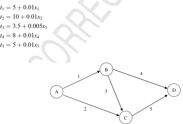
364 To illustrate and confirm the results of section 4 consider the five-link network shown inFig. 4
365 (that has the same topology as that in Yang, 1999). There is a single O–D pair from node A to 366 node D (with a demand of 1000 vph), and three paths: 1–4, 1–3–5, and 2–5. The link cost-flow 367 functions are
t1¼5þ0:01x1 t2¼10þ0:01x2
t3¼3:5þ0:005x3
t4¼8þ0:01x4 t5¼5þ0:01x5
A
B
C
D 1
2
3
4
[image:14.544.73.394.425.643.2]5
UNC
ORREC
TED
PROOF
370 We consider the probit case: that is, Normally distributed perception errors with link variances 371 being fixed and equal to btimes the mean free-flow cost. In carrying out the stochastic loading 372 at any iteration, the algorithm of Donnolly (1973) is used for calculating probabilities from the 373 bivariate Normal distribution. For more general, larger networks, a variety of approximate meth-374 ods can be used to calculate the prs
j values (see Rosa and Maher, 2002).
375 The SUE and SSO solutions are found by using respectively the standard path costscrs j or the
376 marginal social path costscrs j þ
P
axad rs aj
dta
dxaat each iteration when calculating the path choice pro-377 portionsprs
j to produce the auxiliary path flow pattern. The results inTable 1have been obtained,
378 to a high degree of convergence (measured directly by the difference between the current and aux-379 iliary solutions), by an iterative process that optimises the step length along the search direction 380 (y–x) at each iteration (see, for example,Maher and Hughes (1997)).
381 The results are shown inTable 1. It is clear that, as the variance-to-mean ratio bis steadily re-382 duced in value, the SUE solution moves towards the UE solution and the SSO solution moves 383 towards the SO solution, as would be expected.
384 For a value of b= 1, then, the SSO link flows are xSSO= (578.340, 421.660, 119.275, 385 459.066, 540.934) and hence the MSC tolls are s= (5.783, 4.217, 0.596, 4.591, 5.409). By setting 386 up the linear programming problem specified in (11) and (12), the minimal revenue toll set can 387 be found
Maximise z¼578:34D1þ421:66D2þ119:28D3þ459:07D4 þ 540:93D5
subject to:
D1 þ D4c¼0
D1þD3þD5c¼0
D2þD5c¼0
390 and D165.783,D264.217,D360.596, D464.591,D565.409
Table 1
Path flows assigned by SUE and SSO for variousbvalues
h1 h2 h3
SUEb= 1 463.318 144.990 391.692 SUEb= 0.1 500.046 89.525 410.429 SUEb= 0.01 519.977 56.640 423.383 SUEb= 0.001 528.571 41.773 429.656 SUEb= 0.0001 531.750 36.155 432.094 SUEb= 0.00001 532.824 34.244 432.933 UE 533.333 33.333 433.333
UNCORRECTED
PROOF
391 An optimal solution is found to beD= (5.035, 4.217,0.818, 4.591, 5.409) so that the minimal 392 revenue tollss–D= (0.748, 0, 1.414, 0, 0), raising a total revenue of 601 compared with a revenue of 393 10,227 raised from the MSC tolls.
394 9. Summary
395 In this paper, we have formulated the SSO (Stochastic Social Optimum) traffic assignment 396 problem to complement the well-known UE, SO and SUE problems and investigated the relation-397 ships and similarities between them. The formulation is for a general utility-maximisation frame-398 work, which includes as special cases both logit and probit. Under SSO assignment, the total 399 perceived travel cost is minimised with, generally, some users being assigned to paths that are 400 not their personal minimum perceived cost paths. The analysis was developed in two stages. 401 The first stage involved the optimal assignment of users to paths for any given set of path flows 402 h, with the idea of augmented path costsc–din which thedrsj values were such that the flow pattern 403 produced by the stochastic loading matched the required flow pattern, and produced an expres-404 sionzSSO(h) for the minimum total perceived cost. The second stage then investigated the condi-405 tions for the minimisation ofzSSO(h)with respect to the path flowsh. It was shown that under a 406 general utility-maximising framework that includes the two most important cases of logit and pro-407 bit loading, the augmented path costs at the SSO solution were the marginal social costs, and 408 hence the relationship of the SSO solution to the SUE is the same as that of SO to UE. In par-409 ticular, the SSO solution can be found by means of an SUE algorithm, by replacing the standard 410 path costs by the marginal social path costs in the stochastic loading; and the toll set that is opti-411 mal in the stochastic case has the same form as that which is optimal in the deterministic case, but 412 evaluated at the SSO flow values instead of the SO flow values. Additionally, for the logit case, an 413 expression for the objective functionzSSO(h) has been derived which has a pleasing symmetry with 414 those for UE, SO and SUE. Finally, a link-based objective function has been formulated for the 415 general utility-maximising case (that includes probit as well as logit), which is similar in form to 416 the SUE objective function of Sheffi and Powell.
417 Acknowledgements
418 The authors are grateful to three referees who provided useful comments and suggestions for 419 improving the clarity of the arguments presented in the paper.
420 References
421 Donnolly, T.G., 1973. Algorithm 462: bivariate normal distribution. Communications of the Association of Computing 422 Machinery 16 (10), 638.
UNC
ORREC
TED
PROOF
426 Rosa, A., Maher, M.J., 2002. Algorithms for solving the probit path-based stochastic user equilibrium traffic 427 assignment problem with one or more user classes. In: Proceedings of the 15th International Symposium on 428 Transportation and Traffic Theory, University of South Australia, Adelaide, 16–18 July.
429 Sheffi, Y., 1985. Urban Transportation Networks: Equilibrium Analysis with Mathematical Programming Methods. 430 Prentice-Hall.
431 Sheffi, Y., Powell, W., 1982. An algorithm for the equilibrium assignment problem with random link times. Networks 432 12, 191–207.
433 Taha, H.A., 1976. Operations Research: an Introduction. Collier Macmillan.
434 Wardrop, J.G., 1952. Some theoretical aspects on road traffic research. Proceedings of the Institution of Civil Engineers 435 11 (1), 325–378.
436 Yang, H., 1999. System optimum, stochastic user equilibrium and optimal link tolls. Transportation Science 33 (4), 437 354–360.