Playing Muller Games in a Hurry∗†
John Fearnley
Department of Computer Science, University of Liverpool Liverpool L69 3BX, United Kingdom
john.fearnley@liverpool.ac.uk
Martin Zimmermann
Lehrstuhl Informatik 7, RWTH Aachen University 52056 Aachen, Germany
zimmermann@automata.rwth-aachen.de
Received (Day Month Year) Accepted (Day Month Year) Communicated by (xxxxxxxxxx)
This work considers a finite-duration variant of Muller games, and their connection to induration Muller games. In particular, it studies the question of how long a finite-duration Muller game must be played before the winner of the finite-finite-duration game is guaranteed to be able to win the corresponding infinite-duration game. Previous work by McNaughton has shown that this must occur afterQnj=1(j!+1) moves, and the reduction from Muller games to parity games gives a bound ofn·n! + 1 moves. We improve upon both of these results, by giving a bound of 3nmoves.
Keywords: Muller Games; Zielonka’s Algorithm; Winning Strategies. 2010 Mathematics Subject Classification: 91A46, 91A43, 68N30
1. Introduction
In an infinite game, two players move a token through a finite graph, thereby con-structing an infinite path. The winner is determined by a winning condition, which partitions the infinite paths of the graph into winning paths for Player 0 and win-ning paths for Player 1. Many winwin-ning conditions depend on the vertices that are visited infinitely often, i.e., the winner of a play cannot be determined after a finite number of steps. We study the following question: is it possible to give a criterion to define a finite duration variant of an infinite game? Such a criterion has to stop ∗A preliminary version appeared in Proceedings of the First Symposium on Games, Automata, Logic, and Formal Verification (GANDALF 2010), EPTCS 25, 2010, pp. 146-161.
†Parts of this work were carried out while the second author visited the University of Warwick, supported by EPSRC grant EP/E022030/1 and the projectGames for Analysis and Synthesis of Interactive Computational Systems (GASICS)of theEuropean Science Foundation.
a play after a finite number of steps and then declare a winner based on the finite play constructed thus far. It is sound if Player 0 has a winning strategy for the infinite duration game if and only if Player 0 has a winning strategy for the finite duration game.
McNaughton considered the problem of playing infinite games in finite time from a different perspective. His motivation was to make infinite games suitable for “casual living room recreation” [8]. As human players cannot play infinitely long, he envisions a referee that stops a play at a certain time and declares a winner. The justification for declaring a winner is that “if the play were to continue with each [player] playing forever as he has so far, then the player declared to be the winner would be the winner of the infinite play of the game” [8].
Besides this recreational aspect of infinite games there are several interesting theoretical questions that motivate this problem. A sound criterion to stop a play after at most n steps yields a simple algorithm to determine the winner of the infinite game: the finite duration game can be seen as a reachability game on a finite tree of depth at mostnthat is won by the same player that wins the infinite duration game. There exist simple and efficient algorithms to determine the winner in reachability games on trees and thus also to determine the winner of the infinite duration game. Furthermore, if winning strategies for the reachability game can be turned into (small) finite-state winning strategies for the infinite duration game, then this may yield strategies with memory bounds that are better than those obtained through game reductions. This is because the bounds obtained from game reductions ignore the structure of the arena. Therefore, we may be able to improve upon these results in the average case, although the worst case bounds given by Dziembowski, Jurdzi´nski, and Walukiewicz [3] will continue to hold.
Consider the following criterion: the players move the token through the arena until a vertex is visited twice. An infinite play can then be obtained by assuming that the players continue to play the loop that they have constructed, and the winner of the finite play is declared to be the winner of this infinite continuation. If the game is determined with positional strategies for both players, then this criterion is sound: if a player has a positional winning strategy for the infinite game, then this strategy can be used to win the finite version of the game and vice versa.
Therefore, McNaughton considered games that are not positionally determined. Here, the first loop does not determine an entire infinite play, as memory allows a player to make different decisions when a vertex is seen again. Therefore, the players have to play longer before the play can be stopped and analyzed.
0 1 2
Fig. 1. An arenaG.
was visited entirely since the last visit of a vertex that is not in F. In an infinite play, the set of vertices seen infinitely often is the unique setF such that ScF tends
to infinity after being reset to 0 only a finite number of times.
Let G be the arena in Figure 1 (Player 0’s vertices are shown as circles and Player 1’s vertices are shown as squares) and consider the Muller game
G = (G,F0,F1) with F0 = {{0,1,2},{0},{2}}. In the play 100122121 the score for the set{1,2} is 3, as it was seen thrice (i.e., with the infixes 12, 21, and 21). Note that the order of the visits to the elements ofF is irrelevant and that it is not required to close a loop in the arena. The following winning strategy for Player 0 bounds the scores of Player 1 by 2: arriving from 0 at 1 move to 2 and vice versa. However, Player 0 cannot avoid a score of 2 for Player 1, as either the play prefix 1001 or 1221 is consistent with every winning strategy.
McNaughton proved the following criterion to be sound [8]: stop a play after a score of |F|! + 1 for some set F is reached for the first time, and declare the winner to be the Player isuch that F ∈ Fi. However it can take a large number
of steps for a play to reach a score of|F|! + 1, as scores may increase slowly or be reset to 0. It can be shown that a play must be stopped by this criterion after at mostQ|G|
j=1(j! + 1) steps. Furthermore, there are examples in which it takes at least 1
2
Q|G|
j=1(j! + 1) steps before the criterion declares a winner.
The reduction from Muller games to parity games [5,7] provides another sound criterion. The reduction constructs a parity game of size |G| · |G|!, and since par-ity games are positionally determined, a winner can be declared after the players construct a loop in the parity game. This gives a sound criterion that stops a play after at most|G| · |G|! + 1 steps.
Hence, the threshold of 3 in our main theorem is optimal.
We complement this by proving that a score of 3 must be reached after at most 3|G| steps. Hence, we obtain a better bound than |G| · |G|! + 1 steps and
Q|G|
j=1(j! + 1) steps, which were derived from waiting for a repetition of memory states or McNaughton’s criterion, respectively.
Related work.Usually, the quality of a strategy is measured in terms of mem-ory needed to implement it. However, there are other quality measures of winning strategies. Chatterjee, Henzinger, and Horn have studied a strengthening of parity objectives, where a bound between the occurrences of even colors is required [2]. Another quality measure appears in work on request-response games [6,11], where waiting times between requests and their responses are used to define the value of a play. There it is shown that time-optimal winning strategies can be computed effectively. The maximal score achieved by the opponent is a quality measure for winning strategies in a Muller game. Player 0 prefers plays with small scores for Player 1, which corresponds to not spending a long time in a set of the opponent.
Bernet, Janin, and Walukiewicz used a reduction from parity games to safety games in order to compute the most permissive multi-strategy in a parity game [1]. Such a strategy encompasses the behaviors of all positional winning strategies. Fur-thermore, the reduction also allows us to compute the winning regions in the parity game by computing the winning regions in the safety game.
This paper is structured as follows. Section 2 contains basic definitions and fixes our notation. In Section 3, we introduce the scoring functions, prove some properties about scoring, and define finite-time Muller games. In Section 4, we present Zielonka’s algorithm which is used in Section 5 to prove the main result. Section 6 ends the paper with a conclusion and some pointers to further research.
2. Definitions
The power set of a setSis denoted by 2S and
Ndenotes the non-negative integers. The prefix relation on words is denoted byv, its strict version by @. Given a word
w=xy, definex−1w=y andwy−1=x.
An arena G = (V, V0, V1, E) consists of a finite, directed graph (V, E) and a partition (V0, V1) of V denoting the positions of Player 0 (drawn as circles) and Player 1 (drawn as squares). We require that every vertex has at least one outgoing edge. A setX ⊆V induces the subarenaG[X] = (V∩X, V0∩X, V1∩X, E∩(X×X)), if every vertex inXhas at least one successor inX. A Muller gameG= (G,F0,F1) consists of an arenaGand a partition (F0,F1) of 2V.
A play in Gstarting in v ∈V is an infinite sequence ρ=ρ0ρ1ρ2. . . such that
ρ0 =v and (ρn, ρn+1)∈ E for alln ∈ N. The occurrence set Occ(ρ) and infinity set Inf(ρ) of ρ are given by Occ(ρ) = {v ∈ V | ∃n ∈ Nsuch thatρn = v} and
Inf(ρ) ={v∈V | ∃ωn∈
Nsuch thatρn =v}. We also use the occurrence set of a
allw ∈ V∗ and all v ∈ Vi. The play ρis consistent with σ if ρn+1 = σ(ρ0. . . ρn)
for everyn∈ Nwith ρn ∈Vi. The set of strategies for Playeri is denoted by Πi.
The unique play starting atv ∈V that is consistent with σ∈Πi andτ ∈Π1−i is
denoted by Play(v, σ, τ). A strategyσfor Playeriis positional, ifσ(wv) =σ(v) for everyw∈V∗and everyv∈Vi. Hence, we denote a such a strategy byσ: Vi→V.
A strategy σ for Player i is a winning strategy from a vertex v ∈ V, if every play that starts inv and is consistent withσ is won by Playeri. The strategyσis a winning strategy for a set of verticesW ⊆V, if every play that starts in some
v∈W and is consistent withσis won by Playeri. The winning regionWicontains
all vertices from which Playerihas a winning strategy. A game is determined ifW0 andW1form a partition of V.
Theorem 1 ([5]) Muller games are determined.
Let G = (V, V0, V1, E) be an arena and let X ⊆ V be a set that induces a subarena. The attractor for Playeriof a set F ⊆V in X is AttrXi (F) =
S|V| n=0An
whereA0=F∩X and
An+1=An∪ {v∈Vi∩X| ∃v0∈An such that (v, v0)∈E}
∪ {v∈V1−i∩X | ∀v0∈X with (v, v0)∈E :v0∈An} .
A setX ⊆V is a trap for Player i, if all outgoing edges of the vertices in Vi∩X
lead toX and at least one successor of every vertex inV1−i∩X is in X.
Lemma 2. LetGbe an arena with vertex setV andF, X⊆V such thatX induces a subarena.
(1) Player i has a positional strategy to bring the play from every v ∈ AttrXi (F)
intoF.
(2) The set V \AttrXi (F)induces a subarena and is a trap for Playeri inG.
A strategy as in (1) is called attractor strategy.
3. The Scoring Functions and Finite-time Muller Games
This section introduces the notions that are required to formally define finite-time Muller games. In his study of these games, McNaughton introduced the concept of a score. For every set of vertices F the score of a finite play w is the number of times thatF has been visited entirely sincewlast visited a vertex inV \F.
Definition 3 (Score) For everyF ⊆V we define ScF: V+→Nas ScF(w) = max{k∈N|∃x1, . . . , xk ∈V+ such that
Occ(xi) =F for alli andx1· · ·xk is a suffix ofw} .
Definition 4 (Accumulator) For every F ⊆ V we define AccF: V+ → 2F by
AccF(w) = Occ(x), wherexis the longest suffix ofwsuch thatScF(w) = ScF(wy−1) for every suffixy ofx, andOcc(x)⊆F.
A simple consequence of these definitions is that sets with non-zero score and the accumulators of all sets are all pairwise comparable.
Lemma 5 (cf. Theorem 4.2 of [8]) Let w ∈V+. The sets F with ScF(w)≥ 1 together with the setsAccF(w) for someF form a chain in the subset relation.
Proof. It suffices to show that all such sets are pairwise comparable: let F and
F0 be two sets such that either ScF(w) ≥ 1 or F = AccH(w) for some H ⊆ V
and either ScF0(w)≥1 orF0 = AccH0(w) for someH0⊆V. Then, there exist two
decompositions w= w0w1 and w =w00w01 with Occ(w1) =F and Occ(w01) =F0. Now, eitherw1 is a suffix ofw10 or vice versa. In the first case, we haveF ⊆F0 and in the second caseF0 ⊆F.
Note that Lemma 5 implies that there can be at most |V| sets that have a non-zero score at the same time.
Finally, we define the maximum score function. This function maps a subset
F ⊆2V and a playρto the highest score that is reached duringρfor a set inF.
Definition 6 (MaxScore) For every F ⊆ 2V we define MaxSc
F: V+∪Vω →
N∪ {∞}by MaxScF(ρ) = maxF∈FmaxwvρScF(w).
To illustrate these definitions, consider the play w= 12210122 in the arena G
shown in Figure 1, and the setF ={1,2}. We have that ScF(w) = 1, because 122 is
the longest suffix ofwthat is contained in F, and the entire set{1,2} is seen once during this suffix. We have AccF(w) = {2}, because only vertex 2 has been seen
since the score ofF increased to 1. On the other hand, we have MaxSc{F}(w) = 2
because the prefixw0= 1221 ofwhas ScF(w0) = 2.
McNaughton proposed that scores should be used to decide the winner in a finite-time Muller game. As soon as a threshold score ofkfor some setF is reached, the play is stopped and ifF ∈ Fithen Playeriis declared the winner. The next lemma shows that this is sufficient to ensure that the game always terminates.
Lemma 7. Let k∈N. Everyw∈V∗ with|w| ≥k|V| satisfiesMaxSc2V(w)≥k.
Proof. We show by induction over|V| that every wordw ∈ V∗ with |w| ≥k|V|
contains an infix x that can be decomposed as x= x1· · ·xk where every xi is a
non-empty word with Occ(xi) = Occ(x). This implies MaxSc2V(w)≥k.
The claim holds trivially for |V| = 1 by choosing x to be the prefix of w of lengthk andxi=sfor the single vertex s∈V. For the induction step, consider a
decomposition of an infix ofv with the desired properties. Otherwise, every infixx
ofw of length kn contains every vertex of V at least once. Let xbe the prefix of
lengthkn+1 of w and letx =x1· · ·xk be the decomposition of xsuch that each
xi is of length kn. Then, we have Occ(xi) = Occ(x) = V for all i. Therefore, the
decomposition has the desired properties.
Lemma 7 implies that a finite-time Muller game with threshold k must end after at most k|V| steps. We show that this bound is tight. For every k > 0 we
inductively define a word over the alphabet Σn={1, . . . , n} byw(k,1)= 1k−1 and
w(k,n)= (w(k,n−1)n)k−1w(k,n−1). The wordw(k,n)has lengthkn−1, and it can also be shown that MaxSc2Σn(w(k,n)) =k−1. This can easily be turned into a game
where Player 1 loses, but can producew(k,n) to avoid losing for as long as possible. Finally, to declare a unique winner in every play of a finite-time Muller game we must exclude the case where two sets hit scorekat the same time. McNaughton observed that this cannot happen.
Lemma 8 ([8]) Let k, l ≥ 2, let F, F0 ⊆ V, let w ∈ V∗ and v ∈ V such that
ScF(w)< k andScF0(w)< l. If ScF(wv) =k andScF0(wv) =l, thenF =F0.
We can now define a finite-time Muller game. Such a game G = (G,F0,F1, k) consists of an arenaG= (V, V0, V1, E), a partition (F0,F1) of 2V, and a threshold
k≥2. By Lemma 7 we have that every infinite play must reach scorek for some set F after a bounded number of steps. Therefore, we define a play for the finite-time Muller game to be a finite pathw=w0· · ·wn with MaxSc2V(w0· · ·wn) =k,
but MaxSc2V(w0· · ·wn−1)< k. Due to Lemma 8, there is a unique F ⊆V such
that ScF(w) =k. Player 0 wins the play wifF∈ F0 and Player 1 wins otherwise. The notions of strategies and winning regions can all be redefined for finite games. Applying a result of Zermelo to finite-time Muller games yields the following lemma.
Lemma 9 ([9]) Finite-time Muller games are determined.
In fact, McNaughton considered a slightly different definition of a finite-time Muller game. Rather than stopping the play when the score of a set reaches the global threshold k, in his version the play is stopped when the score of a set F
reaches|F|! + 1. He obtained the following result.
Theorem 10 ([8]) If Wi is the winning region of Player i in a Muller game
(G,F0,F1), and Wi0 is the winning region of Playeri in McNaughton’s finite-time Muller game, thenWi=Wi0.
Adapting the proof of Lemma 7 one can show that a play in this version is stopped after at mostQ|G|
j=1(j! + 1) steps. Furthermore, adapting the construction of the lower boundsw(k,n) above, one can also show that there are wordswn∈Σ∗n
such that|wn| ≥ 12
Q|G|
j=1(j! + 1) and MaxSc{F}(wn)<|F|! + 1 for every F ⊆Σn.
corre-0 1 2 3
Fig. 2. The arenaG.
sponding finite-time Muller game with thresholdkhave the same winning regions. As the singleton set{v} has a score of 1 as soon as a play starts inv, the thresh-old 1 is obviously too small. We finish this section by proving that 3 is the smallest possible threshold for which this equivalence can hold. The rest of this paper is dedicated to showing that it does indeed hold for threshold 3.
Theorem 11. There is a Muller game (G,F0,F1) with winning region W0 and
corresponding finite-time Muller game(G,F0,F1,2) with winning region W00 such
thatW06=W00.
Proof. Consider the arenaGin Figure 2 with F1={{0,1,2},{0,2,3}}. The fol-lowing strategy σis winning for Player 0 from every vertex: at vertex 2 alternate between moving to 1 and to 3. Every playρconsistent withσeither ends up in the loop between 0 and 1 or visits every vertex infinitely often. In both cases,ρis won by Player 0.
On the other hand, Player 1 has a winning strategy from vertex 3 in (G,F0,F1,2): starting at 3, Player 1 moves to 0 and then 2. Now, if Player 0 moves to 3, Player 1 answers by moving to 0 and 2. The resulting play 302302 is won by Player 1, as the set {0,2,3} ∈ F1 has reached a score of 2 and no set of Player 0 has reached a score of 2. If Player 0 moves to 1, then Player 1 answers by moving to 0, 1, and then to 2, which gives the play 3021012 that is also won by Player 1.
4. Zielonka’s Algorithm For Muller Games
This section presents Zielonka’s algorithm for Muller games [10], a reinterpretation of an earlier algorithm due to McNaughton [7]. Our notation mostly follows [3,4]. The internal structure of the winning regions computed by the algorithm is used in Section 5 to define a strategy that bounds the scores of the losing player by 2.
As we consider uncolored arenas, we have to deal with Muller games where (F0,F1) is a partition of 2V
0
for some finite set V0 ⊇V, as the algorithm makes recursive calls for such games. This does not change the semantics of Muller games, as we have Inf(ρ)⊆V for every infinite play ρ.
We begin by introducing Zielonka trees, a representation of winning conditions (F0,F1). Given a family of setsF ⊆2V
0
andX ⊆V0, we defineFX={F∈ F |
F ⊆X}. Given a partition (F0,F1) of 2V
0
, we define (F0,F1)X = (F0X,F1
Definition 12 (Zielonka tree [3]) For a winning condition(F0,F1)defined over
a set V0, its Zielonka tree ZF0,F1 is defined as follows: suppose that V 0 ∈ Fi
and let V0
0, V10, . . . , Vk0−1 be the ⊆-maximal sets in F1−i. The tree ZF0,F1 con-sists of a root vertex labelled byV0 with k children which are defined by the trees Z(F0,F1)V00, . . . ,Z(F0,F1)Vk−0 1.
For every Zielonka treeT, we define RtLbl(T) to be the label of the root inT, we define BrnchFctr(T) to be the number of children of the root, and we define Chld(T, j) for 0 ≤ j < BrnchFctr(T) to be the j-th child of the root. Here, we assume that the children of every vertex are ordered by some fixed linear order.
The input of Zielonka’s algorithm (see Algorithm 1) is a finite arena G with vertex setV and the Zielonka tree of a partition (F0,F1) of 2V
0
for some finite set
V0 ⊇ V. For the sake of exposition, we assume that RtLbl(ZF0,F1) ∈ F1 in the
subsequent paragraphs, which implies that Zielonka’s algorithm choosesito be 1. If this is not the case then the roles of the two players can be swapped. The same assumption is made in Section 5. The algorithm computes the winning regions of the players by successively removing parts of Player 0’s winning region (the sets
U0, U1, U2, . . .). By doing this, the algorithm computes an internal structure of the winning regions that is crucial to proving our results in the next section.
Algorithm 1Zielonka(G,ZF0,F1).
i:= The indexj such that RtLbl(ZF0,F1)∈ Fj k:= BrnchFctr(ZF0,F1)
if The root ofZF0,F1 has no childrenthen Wi=V;W1−i=∅
return(W0, W1)
end if
U0:=∅;n:= 0
repeat n:=n+ 1
An:= AttrV1−i(Un−1) Xn:=V \An
Tn := Chld(ZF0,F1, n modk) Yn:=Xn\AttriXn(V \RtLbl(Tn))
(Wn
0, W1n) := Zielonka(G[Yn], Tn)
Un:=An∪W1n−i
untilUn=Un−1=· · ·=Un−k
Wi=V \Un;W1−i=Un
[image:9.595.114.489.436.690.2]return(W0, W1)
0-Un−1
AttrV0(Un−1)
V \RtLbl(Tn)
AttrXn
1 (V \RtLbl(Tn))
[image:10.595.113.487.175.264.2]W0n W1n
Fig. 3. The sets computed by Zielonka’s algorithm.
attractor ofUn−1 also belong toW0. After removing these vertices from the arena, the algorithm also removes the vertices in the 1-attractor of V \RtLbl(Tn). The
remaining vertices form a subarena whose vertex set is a subset of RtLbl(Tn). Hence,
the algorithm can recursively compute the winning regionsWn
i in this subarena with
Zielonka tree Tn. By construction, the winning region W0n is also a subset of the winning region W0, and so the algorithm can move into the next iteration with
Un =An∪W0n. The algorithm only terminates when the size of the set Un does
not increase fork= BrnchFctr(ZF0,F1) consecutive iterations.
The execution of Zielonka’s algorithm gives us a structure for W0 and W1 that we use in Section 5. The set W0 is partitioned into the attractors given by the sets An \Un−1, and the recursively computed winning regions given by the
setsW0n. On the other hand, the structure of W1 is given by the finalk iterations of the algorithm. In each of these iterations, the algorithm computes an attractor AttrXn
1 (V \RtLbl(Tn)), where Xn = W1, and it recursively computes a winning region Wn
1. The attractor and the winning region are a partition of the set W1. Since we haveTn = Chld(ZF0,F1, nmodk), the finalkiterations of the algorithm
givek distinct partitions, one for each child of the root of the Zielonka tree.
Theorem 13 ([10]) Algorithm 1 terminates with a partition (W0, W1), where
Player0has a winning strategy forW0and Player1has a winning strategy forW1. Zielonka’s winning strategies are defined inductively: Player 0 plays the attractor strategy to Un−1 on each set An\Un−1, and the recursively computed winning strategy on each setW0n. Every play consistent with this strategy must eventually be contained within one of the setsWn
0, hence the strategy is winning for Player 0. Player 1 plays using a cyclic counter cranging over 0, . . . , k−1: supposec=j
and letn be the index at which the algorithm terminated. InW1n−j, the strategy plays according to the recursively computed winning strategy. If Player 0 chooses to leaveW1n−j, then the strategy starts playing an attractor strategy to reachV \
RtLbl(Tn−j). Once this set has been reached, the countercis incremented modulok,
and the strategy begins again. There are two possibilities for a play consistent with this strategy: if it stays from some point onwards in someW1n−j, then it is winning by the inductive hypothesis. Otherwise, it visits infinitely many vertices in V \
0 1 2 3 · · · n
Fig. 4. The arenaGnfor Lemma 14.
implies that the infinity set of the play is not a subset of any RtLbl(Chld(ZF0,F1, j)).
Hence, it is inF1 and the play is indeed winning for Player 1.
We continue by showing that these winning strategies do not bound the score of the opponent by a constant.
Lemma 14. There exists a family of Muller gamesGn= (Gn,F0n,F1n)with|Gn|=
n+ 1and|Fn
0|= 1such that W0=V, butMaxScFn
1(Play(v, σ, τ)) =n, whereσis Zielonka’s strategy,v∈V, andτ∈Π1.
Proof. Let Gn = (Vn, Vn,∅, En) with Vn = {0, . . . , n}, En = {(i+ 1, i) | i <
n}∪{(0, n),(1, n)}(see Figure 4), andFn
0 ={Vn}. The Zielonka tree for the winning condition (Fn
0,F1n) has a root labeled byVn andn+ 1 children that are leaves and
are labeled byVn\ {i}for everyi∈Vn. Assume the children are ordered as follows:
Vn\ {0}<· · ·< Vn\ {n}. Zielonka’s strategy forGn, which depends on the ordering
of the children, can be described as follows. Initialize a counterc:= 0 and repeat: (1) Use an attractor strategy to move to vertexc.
(2) Incrementcmodulon+ 1. (3) Go to 1.
This strategy is winning from every vertex. Now assume a play consistent with this strategy has just visited 0. Then, it visits all vertices 1, . . . , n in this order by cycling through the loopn, . . . ,1 exactlyn times. Hence, the score for the set
{1, . . . , n} ∈ F1 is infinitely oftenn.
By contrast, Player 0 has a positional winning strategy forGn that bounds the opponents scores by 2 (and even 1). The reason the strategy described above fails to do this is that it ignores the fact that all other vertices are visited while moving to the vertex 0. In the next section we construct a strategy that recognizes such visits, and it turns out that this is sufficient to bound the opponent’s scores by 2.
5. Bounding the Scores in a Muller Game
In this section, we prove our main result: the finite-time Muller game with thresh-old 3 is equivalent to the corresponding Muller game.
Theorem 15. IfWiis the winning region of Playeriin a Muller game(G,F0,F1),
and Wi0 is the winning region of Player i in the finite-time Muller game
To prove Theorem 15, we show that if a player has a winning strategy for the Muller game, then this player also has a winning strategy for the Muller game that bounds the scores of the opponent by 2. Since the player could use this strategy in order to win the finite Muller game with threshold 3, this implies that fori∈ {0,1}
we have Wi ⊆ Wi0. Since W0 and W1 partition the set of vertices, this fact is sufficient to prove Theorem 15. Note that this actually proves a stronger statement: for every thresholdk≥3 the finite-time Muller game (G,F0,F1, k) is equivalent to the Muller game (G,F0,F1).
The rest of this section is dedicated to proving the following lemma.
Lemma 16. Player i has a winning strategy σ for her winning region Wi in a Muller game G = (G,F0,F1) such that MaxScF1−i(Play(v, σ, τ)) ≤ 2 for every vertexv∈Wi and every τ∈Π1−i.
In Lemma 14 we saw that the strategies computed by Zielonka’s algorithm do not necessarily satisfy the property required by Lemma 16. Our task is to produce strategies that do bound the opponent’s scores by 2. Our strategies are similar in structure to those that are produced by Zielonka’s algorithm, but we must take much more care to ensure that the properties required by Lemma 16 are satisfied.
The winning strategies produced by Zielonka’s algorithm have a recursive struc-ture, which means that a winning strategyσfor a set of verticesW often proceeds by playing a recursively computed winning strategyσ0for a set of verticesW0⊂W. For example, the two players could construct a pathv0. . . vn, wherevn∈W0, and
thenσcould start executingσ0 with the starting vertexvn. However, the vertexvn
may not be the first point at which the play entered the setW0, and there could be a suffixvmvm+1. . . vn of the play such that each vertex in the suffix is contained in
W0. The strategies produced by Zielonka’s algorithm ignore this suffix, because it is not relevant when we only want to construct a winning strategy.
By contrast, when we want to construct a winning strategy that satisfies the properties given by Lemma 16, this suffix turns out to be vitally important. We now give some definitions that allow us to work with such suffixes. Firstly, we redefine the notion of a play. Previously we had that a play begins at a starting vertex, but now we allow a play to begin with a finite initial path over which the players have no control. This new definition is useful, because it allows strategies to base their decisions on the properties of the finite initial path.
Definition 17 (Play) For a non-empty finite path w =w0· · ·wm and strategies
σ∈Πi,τ ∈Π1−i, we define the infinite playPlay(w, σ, τ) =ρ0ρ1ρ2· · · inductively
byρn=wn for0≤n≤m and forn > mby
ρn= (
σ(ρ0· · ·ρn−1) ifρn−1∈Vi,
τ(ρ0· · ·ρn−1) ifρn−1∈V1−i.
was recursively applied. Therefore, we have some control over the form that these paths take. We construct our strategy so that every path passed to a recursive strategy has the following property.
Definition 18 (Burden) Let F ⊆ 2V0. A finite path w is an F-burden if
MaxScF(w) ≤ 2 and for every F ∈ F either ScF(w) = 0 or ScF(w) = 1 and
AccF(w) =∅.
A pathwsatisfies the criteria of a burden if it has the following two properties. Firstly, the requirement that MaxScF(w) ≤ 2 means that the score of every set F∈ F must be bounded by 2 atevery point along the pathw. Secondly, the score of each setF ∈ F at the end of the path must either be 0 or 1. Additionally, if the score is 1, then the accumulator of this set must be empty. In other words, while the scores are allowed to reach 2 during the path, we insist that they satisfy a more restricted condition at the end of the path.
Before we begin proving Lemma 16, we state a useful property of burdens that is applied when we pass burdens to recursively computed strategies.
Remark 19. Let F0 ⊆ F. Every suffix of anF-burden is an F0-burden.
We are now ready to prove Lemma 16. We assume that RtLbl(ZF0,F1)∈ F1. If
this is not the case then the roles of the two players can be swapped. The proof is an induction over the structure of the Zielonka tree. The inductive hypothesis is that, if Zielonka’s algorithm computes the partition into winning regions as (W0, W1), then Playerihas a winning strategy for the setWi that bounds the scores of every
set inF1−i by 2, even if the play starts with anF1−i- burden.
We begin with the base case of the induction, which occurs when the Zielonka tree is a leaf. Since we assume RtLbl(ZF0,F1)∈ F1, we must have that W1 =V.
Therefore, Player 0 can be ignored in this proof.
Lemma 20. Let (G,F0,F1)be a Muller game with vertex set V such that ZF0,F1 is a leaf. Then, Player 1 has a strategy τ such that MaxScF0(Play(wv, σ, τ))≤ 2 for every strategyσ∈Π0 and every F0-burdenwv withv∈V.
Proof. AsZF0,F1is a leaf and RtLbl(ZF0,F1)∈ F1by assumption, we haveF0=∅.
Hence, any strategyτ for Player 1 guarantees MaxScF0(Play(wv, σ, τ))≤2.
For the inductive step, we give two proofs: one for the set W0, and the other for the setW1. We begin with the proof for the set W0. The structure of W0, as computed by Zielonka’s algorithm, is shown in Figure 5. Recall that the set W0 consists of a number of sets Wn
0, which are winning subregions of W0 that have been recursively computed by the algorithm. We denote the recursively computed winning strategy forW0n asσnR. This strategy satisfies the inductive hypothesis, so we know that MaxScF1W0n(Play(wv, σ
R
n, τ))≤2 for every strategy τ of Player 1
W1
[image:14.595.121.466.175.234.2]0 A2\U1 W02 A3\U2 W03
Fig. 5. The structure ofW0. The dashed line shows an example play according toσ∗.
We can now construct our proposed winning strategy. This strategy is similar to the one that is constructed by Zielonka’s algorithm, but our strategy is careful to pass the appropriate finite path to the recursively computed strategyσnR. For
every pathwand every vertexv, we define:
σ∗(wv) =
σnR(w0v) ifv∈W0n andw0 is the longest suffix ofwwith Occ(w0)⊆Wn
0,
σA
n(v) ifv∈An\Un−1.
Note that σ∗ passes the complete suffix of wv that is contained inWn
0 to σnR.
Applying Remark 19 yields, that if wv is an F1 W0n-burden, then w0v is also an F1 W0n-burden. This allows us to apply the inductive hypothesis for σnR in
the following proof, which shows thatσ∗ has the property required by Lemma 16. Therefore, the next lemma proves the part of the inductive step that deals withW0.
Lemma 21. For everyF1W0-burdenwv withv∈W0 and every strategyτ∈Π1
we haveMaxScF1W0(Play(wv, σ
∗, τ))≤2.
Proof. The sets U1 ⊆ U2 ⊆ · · · ⊆ Un form a sequence of hierarchical traps
for Player 1. This means that once Play(wv, σ∗, τ) enters a set Uj, it may never
again visit a vertex in V \ Uj. Therefore, we can represent Play(wv, σ∗, τ) as
wanwnan−1wn−1. . . akwk, wherewis the burden without its last vertex, aj is the
portion of the play after w that is contained in Aj\Uj−1, and wj is the portion
of the play afterwthat is contained inW0j. One or both of these infixes could be empty, and the portion wk contains the infinite suffix of the play. We prove the
claim by induction over this decomposition. The base case follows from the fact thatwv is anF1W0burden, and therefore MaxScF1W0(w)≤2.
We have two cases to consider. Firstly we must prove that if we have MaxScF1W0(wanwn. . . aj) ≤ 2, then we have MaxScF1W0(wanwn. . . ajwj) ≤2.
Here we assume thatwj is nonempty, as the claim trivially holds if wj =ε. Let s
be the first vertex ofwj and letF ∈ F1W0. If F contains at least one vertex in
W0\W
j
0, then the score of F can increase by at most one during the portionwj,
because the play is confined to the set W0j. Since wv is a burden, we must have ScF(wv)≤1. Sinceanwn. . . ajdoes not visit the setW
j
0, and since AccF(wv) =∅in
case ScF(wv) = 1, we must therefore have ScF(wanwn. . . aj)≤1. Thus, even if the
W1j
AttrW1
1 (W1\RtLbl(Tj))
[image:15.595.120.465.175.233.2]W1\RtLbl(Tj)
Fig. 6. The structure ofW1with respect toTj. The dashed line indicates a part of a play according toτ∗between two change points.
wj. Finally, we consider the sets F ⊆W0j. In this case the claim follows from the inductive hypothesis given by Lemma 16 for the recursively computed strategyσR
j.
However, to invoke the inductive hypothesis, we must have thatwanwn. . . ajs is
anF1 W
j
0-burden. If anwn. . . aj is non-empty, then this holds, because then we
have ScF(wanwn. . . aj) = 0 for every setF ⊆W0j. This implies thatwanwn. . . ajs
is indeed anF1W0j-burden. On the other hand, ifanwn. . . aj is empty, then we
have s=v. Thus, as wanwn. . . ajs=wv is an F1W0-burden by assumption, it is also anF1W0j-burden.
Secondly, we must prove that if MaxScF1W0(wanwn. . . wj+1) ≤ 2, then
MaxScF1W0(wanwn. . . wj+1aj) ≤ 2. Let F ∈ F1 W0. If F contains a vertex
inW0\(Aj\Uj−1), then the score ofF must remain below 2 for exactly the same reasons as in the previous case. Otherwise, ifF ⊆Aj\Uj−1, then we claim that
the score ofF can rise to at most 2 during the portion aj. By construction of the
decomposition we have that the score ofF is at most 1 at the start of the portionaj.
It is easy to show that if an attractor strategy is played, then every vertex in the attractor can be seen at most once. This implies that the score ofF can increase to at most 2 duringaj.
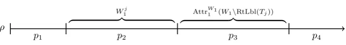
We now turn our attention to the setW1. Letk= BrnchFctr(ZF0,F1). The last k iterations of Zielonka’s algorithm produce for each child Tj = Chld(ZF0,F1, j)
with 0 ≤ j ≤ k−1 an instance of the situation depicted in Figure 6. The set AttrW1
1 (W1\RtLbl(Tj)) has an associated attractor strategyτjA, and the set W j
1 has a recursively computed winning strategyτR
j . This strategy satisfies the inductive
hypothesis, so we know that MaxScF
0W1j
(Play(wv, σ, τR
j ))≤2 for every strategyσ
of Player 0 inG[W1j] and everyF0W1j-burdenwv withv∈W
j
1.
Figure 6 shows the outcome when Player 1 playsτjRandτjA. The play remains in the setW1j until Player 0 chooses to leave, at which point the play is forced to visit some vertex inW1\RtLbl(Tj). Once the play entersW1\RtLbl(Tj), a new index
j0 6=j is selected, and τR
j0 and τjA0 is played. The strategy produced by Zielonka’s
algorithm choosesj0 to bej+ 1 modk, and Lemma 14 shows that this method does not bound the scores of the losing Player by 2. Our goal is to provide a method for choosing a new index that does bound the scores of the opponent by 2.
that this property still holds even if we restrict ourselves to sets inF0. We define the indicator function of a play to be the function that selects the maximal element of this chain, when it is restricted to sets inF0. For every playwwe define:
Ind(w) = [
F∈F0:
ScF(w)>0
F ∪ [
F∈F0
AccF(w) .
The next lemma gives an important property that is used in our index selection method: there is always some child whose label contains the indicator.
Lemma 22. For every play w, there is some j in the range 0 ≤ j ≤ k−1 such thatInd(w)⊆RtLbl(Tj).
Proof. Lemma 5 implies that there is a maximal set C such that Ind(w) = C, with either ScC(w) > 0 or AccF(w) =C for some F ∈ F0 with C ⊆ F. Hence, Ind(w)⊆F for someF ∈ F0, and, by definition ofZF0,F1, there is some child of
the root labeled by RtLbl(Tj) such thatF ⊆RtLbl(Tj).
When a new child must be chosen, our strategy chooses one whose label contains the value of the indicator function for the play up to that point. Lemma 22 implies that such a child must always exist. It is also critically important that this condition is used when picking the child in the first step, which is why we had to introduce the concept of a burden.
We can now formally define this strategy. The strategy uses an auxiliary function
c : W1∗ → {0,1, . . . , k−1,⊥} that specifies which child the strategy is currently considering. For each playw, if c(w) =j then the strategy follows τA
j and τjR. If
c(w) =⊥then the strategy moves arbitrarily.
We begin by defining the function c. This definition encompasses the idea that the strategy should always choose a child that contains the indicator. Therefore, we definec(ε) =⊥, and for every playwand every vertexv we define:
c(wv) =
c(w) ifv∈RtLbl(Tc(w)),
j ifv /∈RtLbl(Tc(w)), Ind(wv)6=∅ andj minimal with Ind(wv)⊆RtLbl(Tj),
⊥ ifv6∈S
0≤j≤k−1RtLbl(Tj).
Note thatcis defined for everywv, as Ind(wv) =∅impliesv6∈S
0≤j≤k−1RtLbl(Tj).
We can now defineτ∗ forW1 as:
τ∗(wv) =
τR
j (w0v) ifc(wv) =j, v∈W j
1 andw0 is the longest suffix ofwwith Occ(w0)⊆Wj
1,
τjA(v) ifc(wv) =j, v∈RtLbl(Tj)\W1j,
x ifc(wv) =⊥wherex∈W1 with (v, x)∈E.
ρ
p1 p2 p3 p4
W1j
z }| {
AttrW1
1 (W1\RtLbl(Tj))
[image:17.595.120.472.174.220.2]z }| {
Fig. 7. The decomposition of a play for Lemma 24. The first vertex ofp4 is not in RtLbl(Tj).
W1j-burden. This allows us to apply the inductive hypothesis forτjR in the part of the inductive step that deals with the setW1.
We now prove thatτ∗has the required properties. Our proof uses change points,
which are positions in a play where thec function changes its value.
Definition 23 (Change Point) Let ρ0ρ1ρ2. . . be a play. We say that n∈Nis a
change point inρif c(ρ0ρ1. . . ρn−1)=6 c(ρ0ρ1. . . ρn−1ρn).
In the next Lemma, we prove that if Player 1 plays according to τ∗ starting from a burden, then the play up to the next change pointnis also a burden. Our intention is to use this as part of an inductive proof that every play bounds the scores of the opponent’s sets by 2.
Lemma 24. Let ρ=ρ0ρ1ρ2. . . be a play, and let ρ0. . . ρm be an F0 W1-burden
such thatρis consistent withτ∗from at leastmonwards. Ifnis the smallest change point inρsatisfyingm < n, thenρ0. . . ρn is anF0W1-burden.
Proof. Letj =c(ρ0. . . ρm) be the index of the child that is chosen at the pointρm.
We first provide a proof for the case where j =⊥. By definition this implies that
ρn0 ∈/ RtLbl(Tl) for all n0 in the range m ≤ n0 < n and all l in the range 0 ≤ l ≤ k−1. Therefore, for every F ∈ F0 we must have ScF(ρ0. . . ρn0) = 0 and
AccF(ρ0. . . ρn0) =∅for alln0 in the rangem≤n0 < n. From this, it is easy to see
thatρ0. . . ρn is anF0W1-burden.
For the casej6=⊥we split the playρinto four pieces, as depicted in Figure 7. The piecep1 contains the portion of ρup to and including the point ρm and the
piece p4 contains the portion of ρ after and including the change point ρn. The
piecep2contains the portion ofρbetween the pointsρmandρnthat is contained in
the setW1j, and the piecep3contains the portion ofρbetween the pointsρmandρn
that is contained in the set AttrW1
1 (W1\RtLbl(Tj)). Clearly, we haveρ=p1p2p3p4. We now prove that MaxScF0(p1p2p3) ≤ 2. The scores at position ρn will be
considered later. For the portion p1 the scores are bounded by 2 by assumption. Now, consider a setF ∈ F0. During the portionp2, we know thatτR
j is being played,
and therefore the inductive hypothesis given by Lemma 16 is sufficient to prove the claim for the case where F ⊆W1j. On the other hand, if there is a vertex s ∈F
During the portionp3 we know that the attractor strategyτjA is being played,
which implies that each vertex in AttrW1
1 (W1\RtLbl(Tj)) can be seen at most once
during this portion. Consider a setF ∈ F0. IfF∩AttrW1
1 (W1\RtLbl(Tj)) =∅then
the score ofF is 0 during the portion p3. Therefore, we only need to consider the case where F∩AttrW1
1 (W1\RtLbl(Tj))6=∅. The assumption thatp1 is a burden implies that ScF(p1) ≤ 1. If F ∩W1j = ∅ then the score of F cannot increase during p2, and since p3 never sees the same vertex twice, we have that the score ofF can increase by at most 1 during p3.
IfF∩W1j6=∅, then we consider two cases. If ScF(p1) = 0, then the score ofF
can increase only once duringp2, as the vertex in AttrW1
1 (W1\RtLbl(Tj)) cannot be
visited inp2. Similarly, the score ofFcan increase only once duringp3, as the vertex inW1j cannot be visited inp3. Hence, it can only increase to 2 duringp3. Otherwise, if ScF(p1) = 1 and AccF(p1) =∅, then the score ofF cannot increase duringp2, as
the vertex in AttrW1
1 (W1\RtLbl(Tj)) cannot be visited. Furthermore, the score can
only be increased once duringp3, as no vertex in AttrW1
1 (W1\RtLbl(Tj)) is visited
twice byp3. Therefore, we have shown that MaxScF0(p1p2p3)≤2.
To complete the proof, we must show that for every setF ∈ F0, either we have ScF(p1p2p3ρn) = 0, or we have ScF(p1p2p3ρn) = 1 and AccF(p1p2p3ρn) = ∅. We
split this proof into two cases. Firstly, we consider setsF ∈ F0such that ScF(p1) = 1 and AccF(p1) = ∅. By definition of c we have F ⊆ Ind(p1), and therefore by
definition of our strategy, we must haveF ⊆RtLbl(Tj). Sinceρn∈W1\RtLbl(Tj),
we must haveρn∈/F. This implies that ScF(p1p2p3ρn) = 0.
We now consider the case where ScF(p1) = 0. If ρn ∈F, then ρn ∈/ AccF(p1),
as we have AccF(p1) ⊆ RtLbl(Tj) and ρn ∈/ RtLbl(Tj). Hence, we must have
ScF(p1p2p3) = 0, asp2p3is confined to RtLbl(Tj). Therefore, if ScF(p1p2p3ρn) = 1
then we must have AccF(p1p2p3ρn) = ∅. On the other hand, ifρn ∈/ F then we
must have ScF(p1p2p3ρn) = 0.
Lemma 24 explains why burdens must be passed between recursive strategies. We use Lemma 24 inductively to show that the strategyτ∗ bounds the scores of Player 0 by 2. However, for the base case of this inductive proof to hold, the finite path that was passed to the strategy must satisfy the burden property. The next lemma shows thatτ∗ satisfies the properties required by Lemma 16.
Lemma 25. We have MaxScF0W1(Play(wv, σ, τ
∗))≤2 for every strategyσ∈Π0
and everyF0W1-burdenwv with v∈W1.
Proof. Letρ = Play(wv, σ, τ∗). Since wv is a burden, we can use Lemma 24 in-ductively to show that, if n ≥ |wv| is a change point in ρ, then ρ0ρ1. . . ρn is a
On the other hand, if there is only a finite number of change points, then let n be the final change point in ρ. Since ρ0. . . ρn is a burden, we have that
MaxScF0W1(ρ0· · ·ρn)≤2. Ifc(ρ0· · ·ρn) =jfor somej in the range 0≤j≤k−1,
then we must haveρm∈W1j for everym≥n. This implies thatτ∗followsσjRfrom
the point nonwards. Since ρ0. . . ρn is also an F1 W1j-burden, we can apply the inductive hypothesis given by Lemma 16 to obtain MaxScF0W1(ρ)≤2.
If c(ρ0· · ·ρn) = ⊥, then alsoc(ρ0· · ·ρm) = ⊥ for every m > n. This implies
ρm6∈RtLbl(Tj) for everyjin the range 0≤j≤k−1, and hence ScF(ρ0· · ·ρm) = 0
for everym > nand everyF∈ F0. Therefore, MaxScF0W1(ρ)≤2.
Finally, we can prove Lemma 16, which also completes the proof of Theorem 15.
Proof. Theorem 13 yields that Algorithm 1 is correct, which means that the setsWi
returned are indeed the winning regions of the players. We prove the following stronger statement by induction over the height ofZF0,F1: Playeri has a winning strategy σ for her winning region Wi such that MaxScF1−i(wv, σ, τ)≤2 for every strategy τ ∈ Π1−i and every F1−i Wi-burden wv with v ∈ Wi. This implies
Lemma 16, as the finite playvfor every v∈Wi is anF1−iWi-burden.
For the induction start, apply Lemma 20. In the induction step, use the strategies obtained from the inductive hypothesis to defineσ∗ and τ∗ as above. Lemma 21 guarantees MaxScF1W0(Play(wv, σ
∗, τ)) ≤ 2 for every τ ∈ Π1 and every F
1
W0-burden wv with v ∈ W0. As Play(wv, σ∗, τ) is confined to W0, we also have MaxScF1(Play(wv, σ
∗, τ))≤2 for everyτ∈Π
1 and everyF1W0-burdenwvwith
v∈W0. The reasoning forW1 is analogous and applies Lemma 25. Bothσ∗andτ∗ are winning, as they bound the scores of the opponent by 2.
6. Conclusion
We have presented a criterion to stop plays in a Muller game after a finite amount of time that preserves winning regions. Our bound 3|G|on the length of a play improves
the bound|G| · |G|! + 1 obtained by a reduction to parity games. Furthermore, our techniques show that the winning player can bound the scores of the opponent by 2 and that this bound is tight.
A finite-time Muller game with thresholdkcan be viewed as a reachability game defined over the unraveling of the original arena up to depth at mostk|G|, which
is of doubly-exponential size in|G|. Simple algorithms can be applied to solve this game. Our results also allow us to reduce Muller games to safety games: for each Muller game we can produce a safety game in which Playeri wins if and only if Playeriis able to avoid a score value of 3 for all sets of the opponent.
Acknowledgements. We would like to thank Wolfgang Thomas for bringing McNaughton’s work to our attention and Marcus Gelderie, Michael Holtmann, Marcin Jurdzi´nski, and J¨org Olschewski for fruitful discussions on the topic. Fi-nally, we would like to thank Roman Rabinovich for his help with the counter example for threshold 2.
References
[1] J. Bernet, D. Janin and I. Walukiewicz, Permissive strategies: from parity games to safety games,ITA,36(3) (2002) pp. 261–275.
[2] K. Chatterjee, T. A. Henzinger and F. Horn, Finitary winning in omega-regular games,ACM Trans. Comput. Log.,11(1) (2009).
[3] S. Dziembowski, M. Jurdzi´nski and I. Walukiewicz, How much memory is needed to win infinite games?, inProceedings of the 8th Annual IEEE Symposium on Logic in Computer Science, (IEEE Computer Society, Los Alamitos, CA, 1997), pp. 99–110. [4] S. Dziembowski, M. Jurdzi´nski and I. Walukiewicz, How much memory is
needed to win infinite games?, Unfinished draft of [3]. Available online at http://www.dcs.warwick.ac.uk/∼mju/Papers/DJW98-memory.ps.
[5] Y. Gurevich and L. Harrington, Trees, automata, and games, inProceedings of the 14th Annual ACM Symposium on Theory of Computing, (ACM, New York, 1982), pp. 60–65.
[6] F. Horn, W. Thomas and N. Wallmeier, Optimal strategy synthesis in request-response games, in Proceedings of the 6th International Symposium on Automated Technology for Verification and Analysis, eds. S. Cha, J.-Y. Choi M. Kim and M. Viswanathan, (Springer, Heidelberg, 2008), LNCS vol. 5311, pp. 385–396.
[7] R. McNaughton, Infinite games played on finite graphs,Ann. Pure Appl. Logic65(2) (1993) pp. 149-184.
[8] R. McNaughton, Playing infinite games in finite time, inA Half-Century of Automata Theory, eds. A. Salomaa, D. Wood and S. Yu (World Scientific, Singapore, 2000), pp. 73–91.
[9] E. Zermelo, ¨Uber eine Anwendung der Mengenlehre auf die Theorie des Schachspiels, inProceedings of the 5th Congress of Mathematicians, Vol. 2, eds. E. W. Hobson and A. E. H. Love, (Cambridge Press, Cambridge, 1913), pp. 501–504.
[10] W. Zielonka, Infinite games on finitely coloured graphs with applications to automata on infinite trees,Theor. Comput. Sci.200(1-2) (1998) pp. 135–183.