tooth reconstruction
.
White Rose Research Online URL for this paper:
http://eprints.whiterose.ac.uk/944/
Article:
Bors, A.G. orcid.org/0000-0001-7838-0021, Kechagias, L. and Pitas, I. (2002) Binary
morphological shape-based interpolation applied to 3-D tooth reconstruction. IEEE
Transactions on Medical Imaging. pp. 100-108. ISSN 0278-0062
https://doi.org/10.1109/42.993129
[email protected] https://eprints.whiterose.ac.uk/ Reuse
Items deposited in White Rose Research Online are protected by copyright, with all rights reserved unless indicated otherwise. They may be downloaded and/or printed for private study, or other acts as permitted by national copyright laws. The publisher or other rights holders may allow further reproduction and re-use of the full text version. This is indicated by the licence information on the White Rose Research Online record for the item.
Takedown
If you consider content in White Rose Research Online to be in breach of UK law, please notify us by
Binary Morphological Shape-Based Interpolation
Applied to 3-D Tooth Reconstruction
Adrian G. Bors¸*, Member, IEEE, Lefteris Kechagias, and Ioannis Pitas, Senior Member, IEEE
Abstract—In this paper, we propose an interpolation algorithm
using a mathematical morphology morphing approach. The aim of this algorithm is to reconstruct the -dimensional object from a group of( 1)-dimensional sets representing sections of that object. The morphing transformation modifies pairs of consecutive sets such that they approach in shape and size. The interpolated set is achieved when the two consecutive sets are made idempotent by the morphing transformation. We prove the convergence of the morphological morphing. The entire object is modeled by succes-sively interpolating a certain number of intermediary sets between each two consecutive given sets. We apply the interpolation algo-rithm for three-dimensional tooth reconstruction.
Index Terms—Mathematical morphology, morphing, shape-based interpolation.
I. INTRODUCTION
I
N MANY tasks, we have to extract object information from a group of sparse sets. Particularly, in medical applications, parts of human body are represented by an image sequence of parallel slices. These slices can be acquired by magnetic reso-nance imaging (MRI), computer tomography (CT), or by me-chanical slicing and digitization. Most often, the distance be-tween adjacent image elements within a slice is smaller than the distance between adjacent image elements in two neighboring slices. In such situations, it is necessary to interpolate additional slices in order to obtain an accurate description of the object for volume visualization and processing [1]. There are two main categories of interpolation techniques for reconstructing objects from sparse sets: grey-level and shape-based interpolation.Grey-level interpolation methods employ nearest-neighbor, splines, linear [2], or polynomial interpolation. Other algorithms employ feature matching [3] or homogeneity similarity [4] for determining the direction of interpolation.
Shape-based interpolation algorithms are usually employed on binary images. These interpolation methods consider shape features extracted from the object sets. A distance function from each pixel to the object boundary is considered for interpolation in [5]. In [6], an interpolation–extrapolation algorithm is
intro-Manuscript received May 7, 1999; revised December 11, 2001. This work was supported in part by GSRT and the European Social Fund under Research Project 99ED 599 (PENED 99). The Associate Editor responsible for coordi-nating the review of this paper and recommending its publication was M. W. Vannier. Asterisk indicates corresponding author.
*A. G. Bors¸ was with the Department of Informatics, University of Thessaloniki, Thessaloniki 540 06, Greece. He is now with the Department of Computer Science, University of York, YO10 5DD York, U.K. (e-mail: [email protected]).
L. Kechagias and I. Pitas are with the Department of Informatics, University of Thessaloniki, Thessaloniki 540 06, Greece.
Publisher Item Identifier S 0278-0062(02)02938-5.
duced which has similarities with that from [5]. Other exten-sions of the algorithm described in [5] are proposed in [7] and [8]. Among six different algorithms, the one based on a chamfer distance and using a modified cubic spline was found to provide the best results in [7]. An interpolation algorithm which uses the elastic matching algorithm, spline theory, and surface consis-tency is considered in [9]. Shape-based interpolation methods have been shown to outperform other interpolation methods in [10]. A mixed gray-level and shape-based method is used for interpolation in [11]. Each slice is represented as a surface by a “lifting” procedure. The intermediary slices are obtained by interpolating the resulting surfaces and converting the interpo-lated surface back to an image by a “collapsing” operation.
Mathematical morphology provides a good theoretical frame-work for shape modeling and interpolation [12], [13]. Erosion and dilation are basic morphologic transformation operations. In [14], each slice is eroded until its number of pixels becomes half of the sum of its initial number of pixels and those of the next slice. Morphing based on a distance transform is used for slice interpolation in [15]. Interpolated sets in [16] are generated from a succession of skeletons derived from the matching of two neighboring set skeletons. The skeleton by influence zone (SKIZ) transform employs dilations of the intersection and of the complementary of the union of two neighboring sets [17].
In this paper, we propose a new binary morphological mor-phing approach for interpolation. The mormor-phing transforms two neighboring sets by combinations of dilations and erosions. The transformation is iteratively performed in such a way that the re-sulting sets become more similar to each other with respect to both shape and dimension. We define a distance measure for assessing the difference between the original and the morphed shape. The interpolated set corresponds to the idempotency of the two morphed sets after a certain number of iterations. Idem-potency is achieved when the difference of the morphed sets is zero. The morphing transformation is applied repeatedly on the new stack of interpolated sets until an appropriate object shape is achieved. We employ the morphological morphing approach for reconstructing three-dimensional (3-D) teeth from digitized slices.
This paper is organized as follows. Section II describes the morphological morphing transformation and Section III the in-terpolation algorithm. In Section IV, we provide some experi-mental results. The conclusions of this study are drawn in Sec-tion V.
II. MORPHOLOGICALMORPHING
Let us consider that we are provided with two sets repre-senting two shapes, denoted by and , in an -dimensional
space denoted as . Shape morphing is a technique for con-structing a sequence of sets showing a gradual transition be-tween the two given shapes. In the following, we describe a mor-phological morphing transformation.
The simplest morphological operations are the dilation and erosion [12]. These operations correspond to the Minkowski set addition and subtraction. The dilation of a set by using the structuring element is given by
(1)
where denotes dilation and represents a structuring ele-ment centered onto an eleele-ment of the set . The erosion of a set
by using the structuring element is given by
(2)
where denotes erosion. The most commonly used structuring element is the elementary ball of dimension . The dilation with the elementary ball expands the given set with a uniform layer of elements while the erosion operator takes out such a layer from the given set.
The basic mathematical morphology operations defined above can be used to derive complex processing operations [12], [13]. Let and be the elements of the sets and . Let be an alignment transform that aligns
with , such that we have . The
alignment operation is done according to an -dimen-sional hyperplane [axis for two-dimen-dimen-sional (2-D) sets] using matching of corresponding features or a centering operation. We define the complement (background) of the set by . After alignment, each element will have a corresponding element which may be a member of the other set , or may be part of its background . In [5], algorithms that use distance transforms for morphing interpolated sets by adding or removing layers of elementary units have been proposed. In [17], the SKIZ was used for set and function interpolation. The interpolated set in [17] is obtained by means of successive dilations of the sets and , until idempotency is achieved. However, such an approach does not correspond to a natural morphing of one set into the other one.
The morphing transformation proposed in this paper ensures a smooth transition from one shape set to the other one by means of several sets whose shapes change gradually. First, our trans-formation influences the elements located on the boundary of the set
(3)
where denotes the neighborhood of the element , having the same size and shape as the structuring element . In our morphing operation, the elements of a boundary set are changed differently according to their correspondences on the other given set [18], [19]. These changes are defined in terms of mathematical morphology basic operations such as dilations (1) and erosions (2). We can identify three possible correspon-dence cases for the elements of the two aligned sets. One
situ-ation occurs when the border region of one set corresponds to the interior of the other set. In this case, we apply the morpho-logical operation of dilation to the border elements
If
then perform (4)
where is the structuring element applied on the set and is the boundary of set . A second case occurs when the border region of one set corresponds to the background of the other set. In this situation, we have erosions of the boundary elements
If
then perform (5)
No modifications are performed when both corresponding ele-ments are members of their sets boundary
If
then perform no change (6)
The last situation corresponds to regions where the two sets co-incide locally and no change is necessary, while (4) and (5) cor-respond to morphing transformations.
By including all these local changes, we define the following morphing transformation applied on the set depending onto the set and on the structuring element
(7)
A similar morphing operation is defined onto the set de-pending on the set and on the structuring element
(8)
According to these transformations, the intersection of the two sets is always retained by the morphing operations (4)–(6). One set will be eroded in those regions which corre-spond to the background of the other set while it will dilate in regions which correspond to the interior of the other set. The proposed morphing operation creates a new set which is a subset of .
In the proposed morphing algorithm, a particular situation occurs when the erosion of the first set includes the dilation of the second set
(9)
We can easily observe that, in this case, (7) and (8) simplify to
(10)
(11)
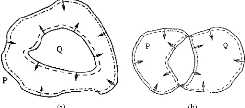
This situation is illustrated for 2-D sets in Fig. 1(a). On the other hand, we have the case when both and contain subsets which are not included in the other set, i.e.,
(a) (b)
Fig. 1. Exemplification of mathematical morphology morphing. The result produced by (8) is represented with dashed lines while the result produced by (7) is represented with dot-dashed lines. Arrows denote dilation and erosion directions; (a)(P 9 B ) (Q 8 B ); (b) P 0 Q 6= andQ 0 P 6= .
The result of the morphing operation applied on either set is a new set. These morphed sets are closer to each other in shape structure and size. In order to measure their similarity, we define a shape distance. Let us consider a structuring element as a ball of radius . Such a structuring element can be obtained from an elementary ball (ball of unit radius) after successive dilations using the elementary ball as the structuring element. Let us define a shape distance between the original set and the morphed set as given by the size of the structuring element . We conventionally assume a positive and a negative direction of morphing. After morphing the sets and with the same structuring element , the distance of the morphed sets to their originating sets is
(12)
where the negative distance has been conventionally assigned. In the general case, this shape distance is not symmetrical
(13)
For isotropic interpolation, we use identical structuring ele-ments, , when morphing the two sets. In this case, each morphed set is equi-distant to its original set. The distance defined in (12) does not depend on the number of elements (pixels in a discretized 2-D space) eroded or added, but on the structural differences between the two shapes that are morphed and on the structuring element size. In the case when the elementary ball is used as structuring element, the shape distance between the original set and its morphing is one.
III. GEOMETRICALLYCONSTRAINEDINTERPOLATION
The morphing operation defined by (7) and (8) is applied it-eratively onto the sets resulted from the previous morphings. The succession of morphing operations creates new sets de-rived from the two initial extremes. With each iteration these sets are closer in shape and size to each other. Three-dimen-sional natural exemplifications of this morphological morphing approach can be found in tree rings and in crystal layer struc-tures. By employing an alignment operation , we can ensure that . The morphing interpolation is based on the following theorem.
Theorem 1: Always we can generate an intermediary set be-tween two sets and , satisfying , by iterating the set transformations defined in (7) and (8) onto their previous it-eration output sets, until idempotency.
Proof: In order to prove the morphing interpolation con-vergence to idempotency, let us consider a set , representing the operation for the two given sets
(14)
We assume that the local morphing termination condition (6) does not occur at the next morphing iteration, which implies that
(15)
In this case, we observe that by considering (7) and (8) and by grouping the resulting set components we obtain
(16)
where for the sake of simplification we dropped out the depen-dency on the elementary structuring element from the expres-sion of the morphing transformation. The morphing rules out-lined in (4)–(6) are employed in the successive morphing opera-tions. We can observe that erosion applies everywhere on the set , excepting for the points which fulfill the condition (6). Such points are not eroded. There is a clear interdependence between the set defined in (14) and the morphological shape distance defined in (12). While with each iteration the set is eroded as it is shown by (16), the distance between the resulting sets, morphed from and , decreases correspondingly
(17)
(a) (b)
[image:5.612.37.291.61.341.2](c) (d)
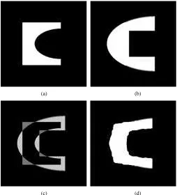
Fig. 2. Shape-based interpolation of two sets. (a) fFirst set. (b) Second set. (c) Difference set. (d) Resulting interpolated set.
happens after iterations. Idempotency after iterations is shown by a zero distance between the resulting morphed sets
(18)
Let us denote by the set obtained at the idempotency of the morphing transformation
(19)
This set has similarities to both initial sets and . The set is equidistant, according to the distance measure defined in (12) to the original sets
(20)
The existence of a set which is equidistant to the initial sets and which corresponds to the case when the set becomes a contour proves the convergence of the morphing Theorem 1.
These results can be easily extended to discrete sets. Elements in such sets consists of hypervoxels in an -dimensional space (pixels for 2-D sets). In order to exemplify this result, we con-sider the 2-D sets from Fig. 2(a) and (b). The initial difference set is shown in Fig. 2(c). After five iterations ( 5) using the structuring element from Fig. 3, we get the inter-polated set , displayed in Fig. 2(d). In this case, the distance between the interpolated set and the original sets is
(21)
which is equal to the number of morphing transformations per-formed by each of these sets until idempotency. The morphing in this example required mostly rectangular to circular shape trans-formations. We can observe that, despite certain discretization errors, the morphing transformations resulted in a good
interpo-Fig. 3. Elementary ball structuring element.
lation result. The interpolated set has similarities to both initial sets, shown in Fig. 2(a) and (b).
All the above assumptions and derivations rely on the fact that we have identical structuring elements for morphing both sets and . In this case, the resulting interpolated set is at equal distance to the given two sets according to (20). However, in certain situations, we may want to interpolate a set, which is at smaller distance to one or another of the given two sets, by using a priori knowledge. We can either use a larger struc-turing element for eroding/dilating the set which should be less similar to the interpolated set, or repeat the morphing for an ad-ditional number of times on that set using the same structuring element. In the case when considering discrete sets, these two approaches can provide slightly different results due to the dis-cretization and approximation of the spherical structuring ele-ment on a discrete grid. Let us assume that we would like an interpolated set whose shape distance ratio to the initial sets is given by
(22)
where we assume a structuring element for morphing and for morphing . The ratio between the radii and of two hyper-spherical structuring elements, is given by
(23)
Let us consider an ordered group of sets , representing cross-sections of a certain object, where rep-resents the total number of sets. The morphing procedure pre-sented above interpolates a new group of sets between each two consecutive sets. In the general case, each new set is equi-dis-tant to the original neighboring sets. The initial and the inter-polated sets will form a new group of sets which can be used for a better visualization of the given 3-D object. We repeat the same procedure on the new pairs of consecutive sets for mod-eling the entire object to a finer detail. After repetitions, the number of interpolated sets generated between two initial sets is . Evidently, there is an upper limit in the number of distinctly interpolated sets generated between two given con-secutive sets. For initial sets we obtain
[image:5.612.382.470.61.149.2]Fig. 4. Diagram describing the interpolation algorithm using morphing of consecutive set pairs.
Fig. 5. Set of tooth slices in resin.
and to choose certain sets, according to their desired intraset dis-tance. In this case, the number of interpolated sets is smaller than
. The intermediate sets, denoted by
for , represent an interpolation between the two initial sets and . Grey-level interpolation can be performed together with the shape interpolation [18]. The pro-cedure of interpolation by successive morphing is exemplified in Fig. 4.
IV. SIMULATIONRESULTS
We have used the proposed morphological morphing interpo-lation algorithm for reconstructing the external and internal 3-D morphology of several teeth. Such an application is of interest in endodontology for representing tooth morphological struc-ture [20]. The examples used in the experiments described in this paper represent normal tooth shapes that are reported in the
[image:6.612.126.468.440.525.2](a)
(b)
[image:7.612.125.471.60.490.2](c)
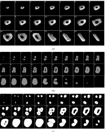
Fig. 6. Segmented and aligned tooth slice sets. (a) Incisor. (b) Premolar (two roots). (c) Molar (three roots).
figure that both canal and outer tooth surface are being smoothly changed from one slice to the next one. A grey-level interpola-tion algorithm [18] was used together with the proposed shape-based interpolation algorithm. This result shows a smooth tran-sition even between slices having large geometrical variations in shape. Three-dimensional reconstructions from two different viewing angles are shown in Fig. 8(a) and (b) for the incisor, in Fig. 8(c) and (d) for the premolar, and in Fig. 8(e) and (f) for the molar, respectively. These volumes are reconstructed from the initial slices shown in Fig. 6. In all these figures, we can observe that the 3-D volumes are well reconstructed. The interpolation of the premolar and of the molar image sequences show the ca-pability of morphing between slices with disconnected sets and those having compact sets. The morphology of the reconstructed teeth is quite accurate despite the fact that a large number of slices has been interpolated.
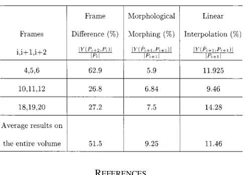
We have compared the mathematical morphological interpo-lation algorithm with a linear interpointerpo-lation algorithm. The linear interpolation algorithm calculates line segments between pixels on object contours of the two slices, in both horizontal and
ver-tical directions. The midpoints of these segments are considered as the interpolated slice contour by this algorithm. We have ap-plied the linear interpolation algorithm on the incisor sequence displayed in Fig. 6(a). We employ a measure for assessing the performance provided by various interpolation algorithms in the following way. Let , and be three original tooth slices and be the result of interpolating and . Let
denote set cardinality. The ratio
Fig. 7. Set of interpolated slices for an incisor.
(a) (c) (e)
(b) (d) (f)
Fig. 8. Three-dimensional views of different reconstructed teeth. (a), (b) Incisor, (c), (d) Premolar. (e), (f) Molar.
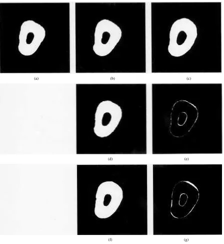
displayed in Fig. 9(d), while in Fig. 9(f) we show the result pro-vided by the linear interpolation approach. The difference be-tween the interpolated and the original set are shown in Fig. 9(e) for the morphological morphing interpolation and in Fig. 9(g) for the linear interpolation. We can observe that the
[image:8.612.74.520.314.659.2](a) (b) (c)
(d) (e)
[image:9.612.74.522.59.546.2](f) (g)
Fig. 9. Slices interpolated by morphological morphing and by linear interpolation from the tenth and twelfth slices of the incisor sequence compared with the real eleventh slice. (a) Tenth slice. (b) Eleventh slice. (c) Twelfth slice. (d) Morphological morphing. (e) Difference set. (f) Linear interpolation. (g) Difference set.
purposes both these volumes are visualized from the same view angle. We can observe that the shape of the molar is better re-constructed by the morphological morphing algorithm than by linear interpolation. These graphical results together with nu-merical results from Table I show that the proposed morpho-logical morphing interpolation algorithm provides good experi-mental results in the case of 3-D tooth reconstruction from dig-itized slices.
V. CONCLUSION
In this paper, we propose a morphological morphing algo-rithm. We consider a group of sets representing sampled object
(a) (b)
Fig. 10. Reconstruction of a 3-D molar by (a) linear interpolation and (b) morphological morphing.
TABLE I
OBJECTIVECOMPARISONMEASUREBETWEENMORPHOLOGICALMORPHING ANDLINEARINTERPOLATIONWHENRECONSTRUCTING ANINCISOR
REFERENCES
[1] G. Lohmann, Volumetric Image Analysis: An Overview. New York: Wiley-Teubner, 1998.
[2] A. Goshtasby, D. A. Turner, and L. V. Ackerman, “Matching of tomo-graphic slices for interpolation,” IEEE Trans. Med. Imag., vol. 11, pp. 507–516, Dec. 1992.
[3] M. Moshfeghi, “Directional interpolation for magnetic resonance an-giography data,” IEEE Trans. Med. Imag., vol. 12, pp. 366–379, June 1993.
[4] W. E. Higgins, C. J. Orlick, and B. E. Ledell, “Nonlinear filtering ap-proach to 3-D grey-scale image interpolation,” IEEE Trans. Med. Imag., vol. 15, pp. 580–587, Aug. 1996.
[5] S. P. Raya and J. K. Udupa, “Shape-based interpolation of multidimen-sional objects,” IEEE Trans. Med. Imag., vol. 9, pp. 32–42, Feb. 1990. [6] P. N. Werahera, G. J. Miller, G. D. Taylor, T. Brubaker, F.
Danesh-gari, and E. D. Crawford, “A 3-D reconstruction algorithm for inter-polation and extrainter-polation of planar cross sectional data,” IEEE Trans. Med. Imag., vol. 14, pp. 765–771, Dec. 1995.
[7] G. T. Herman, J. Zheng, and C. A. Bucholtz, “Shape-based interpola-tion,” IEEE Computer Graphics and Applicat., vol. 12, pp. 69–79, May 1992.
[8] W. E. Higgins, C. Morice, and E. L. Ritman, “Shape-based interpolation of tree-like structures in three-dimensional images,” IEEE Trans. Med. Imag., vol. 12, pp. 439–450, Sept. 1993.
[9] S.-Y. Chen, W.-C. Lin, C.-C. Liang, and C.-T. Chen, “Improvement on dynamic elastic interpolation technique for reconstructing 3-D objects from serial cross sections,” IEEE Trans. Med. Imag., vol. 9, pp. 71–83, Feb. 1990.
[10] G. J. Grevera and J. K. Udupa, “An objective comparison of 3-D image interpolation methods,” IEEE Trans. Med. Imag., vol. 17, pp. 642–652, Apr. 1998.
[11] , “Shape-based interpolation of multidimensional grey-level im-ages,” IEEE Trans. Med. Imag., vol. 15, pp. 881–892, June 1996. [12] J. Serra, Image Analysis and Mathematical Morphology. New York:
Academic, 1982.
[13] I. Pitas and A. N. Venetsanopoulos, Nonlinear Digital Filters: Principles and Applications. Norwell, MA: Kluwer Academic, 1990.
[14] M. Joliot and B. M. Mazoyer, “Three-dimensional segmentation and interpolation of magnetic resonance brain images,” IEEE Trans. Med. Imag., vol. 12, pp. 269–277, June 1993.
[15] B. Luo and E. R. Hancock, “Slice interpolation using the distance trans-form and morphing,” in Proc. Int.. Conf. Digital Signal Processing, San-torini, Greece, 1997, pp. 1083–1086.
[16] V. Chatzis and I. Pitas, “Interpolation of 3-D binary images based on morphological skeletonization,” IEEE Trans. Med. Imag., vol. 19, pp. 699–710, July 2000.
[17] S. Beucher, “Sets, partitions and functions interpolations,” in Proc. Int. Symp. Mathematical Morphology and Its Applications to Image and Signal Processing IV, Amsterdam, Netherlands, June 3–5, 1998, pp. 307–314.
[18] A. G. Bors¸, L. Kechagias, and I. Pitas, “Virtual drilling in 3-D objects reconstructed by shape-based interpolation,” in Lecture Notes in Computer Science, C. Arcelli, L. P. Cordella, and G. Sanniti di Baja, Eds. Capri, Italy, May 2001, vol. 2059, Proc. Int. Workshop Visual Form, pp. 729–738.
[19] , “Shape-based interpolation using morphological morphing,” in Proc. IEEE Int. Conf. Image Processing, vol. II, Thessaloniki, Greece, Oct. 7–10, 2001, pp. 161–164.