Solving Transition-Independent Multi-agent MDPs with Sparse Interactions (Extended version)

Solving Transition-Independent Multi-agent MDPs with Sparse

Interactions

(Extended version)

Joris Scharpff1, Diederik M. Roijers2, Frans A. Oliehoek2,3, Matthijs T. J. Spaan1, Mathijs M. de Weerdt1

1 _{Delft University of Technology, The Netherlands}

2 _{University of Amsterdam, The Netherlands}

3 _{University of Liverpool, United Kingdom}

Abstract

In cooperative multi-agent sequential decision making under uncertainty, agents must coordinate to find an optimal joint policy that maximises joint value. Typical algorithms exploit additive structure in the value function, but in the fully-observable multi-agent MDP (MMDP) setting such structure is not present. We propose a new optimal solver for transition-independent MMDPs, in which agents can only affect their own state but their reward depends on joint transitions. We represent these de-pendencies compactly inconditional return graphs (CRGs). Using CRGs the value of a joint policy and the bounds on partially specified joint policies can be efficiently computed. We propose CoRe, a novel branch-and-bound policy search algorithm building on CRGs. CoRe typically requires less runtime than the available alternatives and finds solutions to previously unsolvable problems.

1

Introduction

When cooperative teams of agents are planning in uncertain domains, they must coordinate to max-imise their (joint) team value. In several problem domains, such as traffic light control [Bakker et al., 2010], system monitoring [Guestrin et al., 2002a], multi-robot planning [Messias et al., 2013] or main-tenance planning [Scharpff et al., 2013], the full state of the environment is assumed to be known to each agent. Suchcentralisedplanning problems can be formalised as multi-agent Markov decision pro-cesses (MMDPs) [Boutilier, 1996], in which the availability of complete and perfect information leads to highly-coordinated policies. However, these models suffer from exponential joint action spaces as well as a state that is typically exponential in the number of agents.

In problem domains with local observations, sub-classes ofdecentralisedmodels exist that admit a value function that is exactly factored into additive components [Becker et al., 2003, Nair et al., 2005, Witwicki and Durfee, 2010] and more general classes admit upper bounds on the value function that are factored [Oliehoek et al., 2015]. In centralised models however, the possibility of a factored value function can be ruled out in general: by observing the full state, agents can predict the actions of others

∗

This article is an extended version of the paper that was published under the same title in the Proceedings of the Thirtieth AAAI Conference on Artificial Intelligence (AAAI16), held in Phoenix, Arizona USA on February 12-17, 2016. The most significant difference is that here a more strict definition of dependent actions, transition influence and, consequentially, the conditional return graphs is given. Furthermore, this version contains additional details and explanations that did not make it into the conference paper due to the page limit.

better than when only observing a local state. This in turn means that each agent’s action should be conditioned on the full state and that the value function therefore also depends on the full state.

A class of problems that exhibits particular structure is that of task-based planning problems, such as the maintenance planning problem (MPP) from [Scharpff et al., 2013]. In the MPP every agent needs to plan and complete its own set of road maintenance tasks at minimal (private) maintenance cost. Each task is performed only once and may delay with a known probability. As maintenance causes disruption to traffic, agents are collectively fined relative to the (super-additive) hindrance from theirjoint actions. Although agents plan autonomously, they depend on others via these fines and must therefore coordinate. Still, suchreward interactionsare typically sparse: they apply only to certain combinations of maintenance tasks, e.g. in the same area, and often involve only a few agents. Moreover, when an agent has performed its maintenance tasks that potentially interfere with others, it will no longer interact with any of the other agents.

Our main goal is to identify and exploit such structure in centralised models, for which we consider transition independentMMDPs (TI-MMDPs). In TI-MMDPS, agent rewards depend on joint states and actions, but transition probabilities are individual. Our key insight is that we can exploit the reward struc-ture of TI-MMDPs by decomposing thereturnsof all execution histories (i.e., all possible state/action sequences from the initial time step to the planning horizon) into components that depend on local states and actions.

We build on three key observations. 1) Contrary to the optimal value function, returns canbe de-composed without loss of optimality, as they depend only on local states and actions of execution se-quences. This allows a compact representation of rewards and efficiently computable bounds on the optimal policy value via a data structure we call theconditional return graph(CRG). 2) In TI-MMDPs agent interactions are often sparse and/or local, for instance in the domains mentioned initially, typically resulting in very compact CRGs. 3) In many (e.g. task-modelling) problems the state space is transient, i.e., states can only be visited once, leading to a directed, acyclic transition graph. With our first two key observations this often gives rise toconditional reward independence, i.e. the absence of further reward interactions, and enables agent decoupling during policy search.

Here we proposeconditional return policy search(CoRe), a branch-and-bound policy search algo-rithm for TI-MMDPs employing CRGs, and show that it is effective when reward interactions between agents are sparse. We evaluate CoRe on instances of the aforementioned MPP with uncertain outcomes and very large state spaces. We demonstrate that CoRe evaluates only a fraction of the policy search space and thus finds optimal policies for previously unsolvable instances and commonly requires less runtime than its alternatives.

2

Related work

Scalability is a major issue in multi-agent planning under uncertainty. In response to this challenge, two important lines of work have been developed. One line of work proposed approximate solutions by imposing and exploiting an additive structure in the value function [Guestrin et al., 2002a]. This approach has been applied in a range of stochastic planning settings, fully and partially observable alike, both from a single-agent perspective [Koller and Parr, 1999, Parr, 1998] and multi-agent [Guestrin et al., 2002b, Meuleau et al., 1998, Kok and Vlassis, 2004, Oliehoek et al., 2013b]. The drawback of such methods is that typically no bounds on the efficiency loss can be given. We focus on optimal solutions, required to deal with strategic behaviour in a mechanism [Cavallo et al., 2006, Scharpff et al., 2013].

et al., 2008, Varakantham et al., 2007]. However, all these approaches are for decentralised models in which actions are conditioned only onlocalobservations. Consequentially, optimal policies for decen-tralised models typically yield lower value than the optimal policies for their fully-observable counter-parts (shown in our experiments).

Our focus is on transition-independent problems, suitable for multi-agent problems in which the effects of activities of agents are (assumed) independent. In domains where agents directly influence each other, e.g., by manipulating shared state variables, this assumption is violated. Still, transition independence allows agent coordination at a task level, as in the MPP, and is both practically relevant and not uncommon in literature [Becker et al., 2003, Spaan et al., 2006, Melo and Veloso, 2011, Dibangoye et al., 2013].

Another type of interaction between agents is through limited (global) resources required for certain actions. While this introduces a global coupling, some scalability is achievable [Meuleau et al., 1998]. Whether context-specific and conditional agent independence remains exploitable in the presence of such resources in TI-MMDPs is yet unclear. Additionally, there exist also methods that exploit reward sparsity and independence but through a reinforcement learning approach identifying ‘interaction states’ [De Hauwere et al., 2012, Melo and Veloso, 2009]. Although these target a similar structure, learning implies that there are no guarantees on the solution quality (until all states have been recognised as interaction states, which implies a brute-force solve of the MMDP).

3

Model

We consider a (fully-observable)transition-independent, multi-agent Markov decision process, or TI-MMDP, with a finite horizon of lengthh, and no discounting of rewards.

Definition 1. A TI-MMDP is a tuplehN, S, A, T,Ri:

N ={1, ..., n}is a set ofnenumerated agents;

S =S1×...×Snis the agent-factored state space, which is the Cartesian product ofnfactored states spacesSi_{(composed of featuresf ∈F, i.e.s}i _={fi

x, fyi, . . .});

A = A1×...×An is the joint action space, which is the Cartesian product of thenlocal action spacesAi;

T(s, ~a,sˆ) = Q

i∈NTi(si, ai,sˆi)defines a transition probability, which is the product of the local

transition probabilities due to transition independence; and

Ris the set of reward functions over transitions that we assume without loss of generality is struc-tured as{Re|e⊆N}. When e = {i}, Ri is the local reward function for agent i, and when

|e| > 1, Re is called an interaction reward. The total team reward per time step, given a joint states, joint action~aand new joint stateˆs, is the sum of all rewards:

R(s, ~a,sˆ) = X

Re_∈R

Re({sj}j∈e,{~aj}j∈e,{sˆj}j∈e). (1)

Two agents iandj are calleddependent when there exists a reward function with both agents in its scope, e.g., a two-agent reward Ri,j_({si_{, s}j_},{ai_{, a}j_},{ˆsi_,ˆsj_{}) could describe the super-additive}

hindrance that results when agents in the MPP do concurrent maintenance on two nearby roads. We focus on problems withsparse interaction rewards, i.e., reward functionsRewith non-zero rewards for a small subset of the local joint actions (e.g.,Aij _⊂Ai_×Aj_{) or only a few agents in its scope. Of course,}

and participating agents (respectivelyαandwin Theorem 1) determine the level of sparsity. Note that this is not a restriction but rather a classification of problems that benefit most from our approach.

The goal in a TI-MMDP is to find the optimal joint policyπ∗ of which the actions~amaximise the expected sum of rewards, expressed by the Bellman equation:

V∗(st) = max ~ at

X

st+1∈S

T(st, ~at, st+1)

_X

Re_∈R

Re(se_t, ~ae_t, se_t+1) +V∗(st+1)

. (2)

At the last timestep there are no future rewards, so V∗(sh) = 0 for every sh ∈ S. Although

V∗(st)can be computed through a series of maximisations over the planning period, e.g. via dynamic

programming [Puterman, 2014], it cannot be written as a sum of independent local value functions without losing optimality [Koller and Parr, 1999], i.e.V∗(s)6=P

eVe,

∗_(se_).

Instead, we factor thereturnsofexecution sequences, the sum of rewards obtained from following state/action sequences, which is optimality preserving. We denote an execution sequence up until time

tasθt = [s0, ~a0, ..., st−1, ~at−1, st]and its return is the sum of its rewards: Pt_x−₌₀1 R(sθ,x, ~aθ,x, sθ,x+1),

where sθ,x,~aθ,x andsθ,x+1 respectively denote the state and joint action at time x, and the resulting

state at timex+ 1in this sequence. A seemingly trivial but important observation is that the return of an execution sequence can be written as the sum of local functions:

Z(θt) = X

Re_∈R

t−1 X

x=0

Re(se_θ,x, ~ae_θ,x, se_θ,x+1), (3)

wherese_θ,x,~ae_θ,xandse_θ,x+1 denote local states and actions fromθtthat are relevant forRe. Contrary to

the optimal value function, (3) is additive in the reward components and can thus be computed locally. Nonetheless, the return of (3) does not directly give us the value of an optimal policy. To compute the expected policy value using (3), we sum the expected return of all future execution sequencesθh

reachable under policyπstarting ats0(denotedθh|π, s0):

Vπ(s0) = X

θh|π,s0

P r(θh)Z(θh) = X

θh|π,s0

Z(θh) h−1 Y

t=0

T(sθ,t, π(sθ,t), sθ,t+1). (4)

Now, (4) is structured such that it expresses the value in terms of additively factored terms (Z(θh)).

However, comparing (2) and (4), we see that the price for this is that we no longer are expressing the optimalvalue function, but that of a given policyπ. In fact, (4) corresponds to an equation forpolicy evaluation. It is thus not a basis for dynamic programming, but it is usable for policy search. Although policy search methods have their own problems in scaling to large problems, we show that the structure of (4) can be leveraged.

In particular, because the return of an execution sequence can be decomposed into additive compo-nents (Eq. 3), we decouple and store these returns locally in conditional return graphs(CRGs). The CRG is used in policy search to efficiently compute (4) when, during evaluation, the transition proba-bilityP r(θ)of an execution sequenceθbecomes known. Moreover, the returns stored in the CRG can be used to bound the expected value of sequences, allowing branch-and-bound pruning. Finally, when constructing CRGs it is possible to detect the absence future reward interactions between agents and thus optimally decouple the policy search.

4

Conditional Return Graphs

(a) (b)

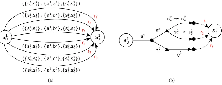
Figure 1: Example of a transition for one agent of a two-agent problem where (a) shows the complete state/transition graph with unique rewardsrx and (b) the equivalent but more compact CRG whenR1

only depends ona2₁.

toi(restricted toRe_{wherei∈e). The setsR}

iare disjoint sub-sets of the reward functionsRsuch that

together they again form the complete set of joint reward functions. Note that such a partitioning can be done in many ways. In our preliminary experiments we observed that for the maintenance planning domain balancing the number of functions per agent works well. Nevertheless, further study is required to establish potentially better or more generic assignment heuristics.

Given such a disjoint partition of rewards, a conditional return graph for agentiis a data structure that represents all possiblelocalreturns, for all possiblelocalexecution histories. Particularly, it is a directed acyclic graph (DAG) with a layer for every staget= 0, . . . , h−1of the decision process. Each layer contains nodes corresponding to the reachable local states si ∈ Si of agentiat that stage. As the goal is to include interaction rewards, the CRG includes for every local statesi, local actionai, and successor statesˆia representation of all transitions(se, ~ae,ˆse)for whichsi ∈se,ai ∈~ae, andsˆi ∈sˆe.

While a direct representation of these transitions captures all the rewards possible, we can achieve a much more compact representation by exploiting sparse interaction rewards, enabling us to group many joint actions~ae leading to the same rewards. Consider a two-agent example N = {1,2} with actionsA1 ={a1}andA2 ={a2, b2, c2}respectively. Both agents have a local reward function, resp.

R1 andR2, and there is one interaction rewardR1,2 that is 0for all transitions but the ones involving joint action{a1, a2}. This could for example be a network cost function of MPP that is non-zero when the maintenance activities corresponding to actions a1 and a2 are performed, e.g. because they take place within close proximity of each other. The interaction rewardR1,2 is assigned to agent1, thus

R1

i = {Ri, R1,2} and of course R2i = {R2}. A naive representation of all rewards would result in

the graph of Figure 1a, illustrating a transition froms1₀ tos1₁ where agent 2may remain in states2₄ or transition to states2₆.

Observe that now there are only three unique rewards (shown in red) whereas there are six possible transitions. Intuitively, all transitions resulting in the same reward should be grouped such that only when the actions/states of other agents influence the reward they should be included in the CRG, resulting in the graph of Figure 1b. To make this explicit, we denote a single transition for agents e ⊆ N by

τe = ({sj}j∈e,{~aj}j∈e,{sˆj}j∈e) = (se, ~ae,ˆse). A local transitionτi is said to be contained inτe,

denotedτi ∈ τe, ifi ∈ e, si ∈ se, ai ∈~ae andsˆi ∈ ˆse. Moreover the set set of all available (joint) transitions can be written as

Te={(se, ~ae,sˆe)|se,sˆe∈ {sj}_j∈e, ~ae∈ {~aj}j∈e, T(se, ~ae, se)>0} (5)

that may interact with the rewardsR_i, assigned to each of the CRGs, given a current local transitionτi= (si_{, a}i_,sˆi_{). An actiona}j _{of agentj 6=iis said to bedependent with respect to local transitionτ}i _{if it}

occurs in one of the available joint transitions that containsτi, its presence influences the interaction reward and there is at least one other action of agentjthat doesnotcause the same interaction reward. The last condition is included to prevent marking all actions as dependent when actually the interaction reward depends on the state transition of agent j. This leads to the following definition of dependent actions:

Definition 2(Dependent Actions). The set of dependent actionsof an agentj ∈ N that may reward-interact with agenti6=jwhen agenti’s local transition isτi = (si, ai,ˆsi)is given by:

A(τi, j) ={aj ∈Aj| ∃Re∈ Ri,∃τe∈ Te,∃bj 6=aj ∈Aj:

τi∈τe∧aj ∈~ae

∧Re(τe)6=Re(τe\ {τj}), s.t.τj ∈τe

∧Re(τe)6=Re(se, ~ae\ {aj} ∪ {bj},sˆe)}

Actions by other agents that are not dependent with respect to a transitionτi, i.e. the actionsAj \ A(τi, j), are (made) anonymous in the CRG for agentivia ‘wildcards’ (e.g.∗2_{of Figure 1b), since they}

do not influence the reward from the functions inRi.

Besides actions, the interaction reward may also be affected by the state transitions of the other agents. This is captured by thetransition influence.1 Its definition is rather similar to that of dependent actions. For a state transitionsj → sˆj of an agentj 6=ito be considered an influence with respect to local transitionτi, both states must be part of a transitionτj such that bothτiandτj are contained in a joint transitionτe, such a transitionτj must have an impact on at least one interaction reward and there must exist at least one other transition of agentjthat does not have the same interaction reward impact. The latter condition is, as before, to prevent all state transitions being marked an influence whereas the interaction reward depends solely on the action. This is formalised by the following definition:

Definition 3. The set of state pairs of an agentjthat may lead to a reward interaction when agenti6=j

perform transitionτi = (si, ai,sˆi)and agentjperforms actionaj ∈Aj concurrently, is known as the

(transition) influence, defined as

Ii(τi, aj) ={(sj,sˆj)∈Sj×Sj| ∃Re∈ R_i,∃τe∈ Te,∃(sj₂,ˆsj₂)= (6 sj,ˆsj)∈Sj×Sj:

τi ∈τe∧τj = (sj, aj,sˆj)∈τe (6)

∧Re(τe)6=Re(τe\ {τj}), s.t.τj ∈τe (7)

∧Re(τe)6=Re(se\ {sj} ∪ {s₂j}, ~ae,ˆse\ {sˆj} ∪ {sˆj₂})} (8)

Finally, for any set of actions Aj of an agent j we define the transition influence of that set with respect to local transitionτi as the union of all influences, orIi(τi, Aj) =S

aj_∈AjIi(τi, aj). This last definition is useful to capture the influence of a wildcard set∗j_{, which occurs when multiple actions}

1_{In [Scharpff et al., 2013] only the set of dependent actions was defined. Although the definition in the paper is correct, for}

some problems it may lead to an unnecessary blow-up of the CRG size. For instance, an interaction reward assigned to agenti

lead to the same state-transition interaction reward. Again, non-influencing state transitions can be grouped. We use the symbolj _{to denote the set of all non-influencing transitions of agent j given a}

local transitionτiand actionaj (or wildcard∗j_).

Given Defs. 2 and 5 above, aconditional return graph(CRG)φifor agentican be defined as follows.

Definition 4 (Conditional Return Graph). Given a disjoint, complete partitioning R = S

i∈NRi of

rewards over agentsi∈N, theConditional Return Graph (CRG)φiis adirected acyclic graphwith for every stagetof the decision process a node for every reachable local statesi ∈Sand for every available local transitionτi = (si, ai,ˆsi)a tree compactly representing all joint transitionsτe = (se, ~ae,sˆe)of the agentse⊆N in the scope ofR_i, ore={i∈N| ∃Re∈ R_i:i∈e}.

The tree consists of two parts: an action treethat specifies all dependent actions and aninfluence treethat contains the relevant local state transitions. For every action ai ∈ Ai of agent i, the state

si is connected to the root nodev_ai of an action tree by an arc labeled with action ai. For every root nodevai, letv =v_ai be the root of an action tree such that it is defined recursively over the remaining

N0 =e\ {i}agents as follows:

A1 IfN0 6=emptysettake somej ∈N0, otherwise stop.

A2 For everyaj ∈ A(τi, j), create an internal node v_aj connected fromv by an arc labeled with the actionaj.

A3 Create one internal nodev∗j to represent all actions of agentjnot inA(τi, j)(if any), connected by an arc labeled by the ‘other action’ wildcard∗j _{from the root nodev.}

A4 For each leaf nodev_aj (orv_∗j) that results from the previous steps, create a sub-tree with N0 =

N0\ {j}andv=vajas its root using the same procedure.

When all action arcs have been created, each leaf nodevaxof the action tree is the root nodeuof an influence tree, whereaxis either the last dependent action or wildcard∗x_{of the agentxthat is visited}

in the last recursion. Starting again fromN0 =e\ {i}:

B1 IfN0 6=emptysettake somej ∈N0, otherwise stop.

B2 If the path from si _{to node u contains an arc labelled with action a}j _{∈ A(τ}i_{, j), create child}

nodesusj_→sˆj to represent all local pairs of state transitions(sj,ˆsj)of agentjin the action influ-enceIi(τi, aj), connected to nodeuby arcs labeledsj →sˆj.

else

The path fromsito nodeucontains the wildcard∗j_{. Create child nodesu}

sj_→sˆj for all pairs of local state transitions(sj,sˆj) ∈ Ii(τi,∗j_{), i.e. the influence of the set of actions represented by∗}j _(all

aj _{∈ A/ (τ}i_{, j)), and connect them touwith arcs labelleds}j _→sˆj_.

B3 If there remains any pair of local states(sj,sˆj) ∈ Sj ×Sj with T(sj, aj,sˆj) > 0 that is not in

Ii(τi, aj)or a pair withP

aj_∈∗jT(sj, aj,sˆj) >0that is not inIi(τi,∗j), depending on the action of agentjon the path to nodeu, create another child nodeuj connected by an arc labeled by the ‘other state pairs’ wildcardj_.

B4 For each leaf nodeu_sj_→ˆsj (oruj) that results from the previous step, create a sub-tree withN0 =

N0\ {j}and rootu=usj_→sˆj (resp.u=uj) repeating the same procedure.

The labels on the path to a leaf node of an influence tree, via a leaf node of the action tree, sufficiently specify the joint transitions of the agents in scope of the functionsRe _{∈ R}i_{, such that we can compute}

the rewardP Re_∈R

iR

e_(se_{, ~a}e_,sˆe_{). Note that for eachR}e _{for which an action is chosen that is not in} A(ai, j)(a wildcard∗j _{in the action tree), the interaction reward must be0by definition (and similarly}

for state transitions inj_).

In Figure 1b an example CRG is illustrated. The local state nodes are displayed as circles; the internal nodes as black dots and action tree leaves as black triangles. The action arcs are labelleda1,a2

and ‘wildcard’∗2_{, whereas transition influence arcs are labelled(s}2

4→s24),(s42 →s26)andj. Note that

Definition 4 captures the general case, but often it suffices to consider transitions(si∪Fe\i, ~ae,ˆsi∪Fˆe\i), where Fe\i is the set of state features on which the reward functions Ri depend. This is a further

abstraction: only feature influence arcs are needed, typically requiring much less arcs (demonstrated later in Figure 2).

Now we investigate the maximal size of the CRGs to derive a theoretical upper bound. Let|Smax|= maxi∈N|Si| and |Amax| = maxi∈N|Ai| denote respectively the maximal individual state and

ac-tion space sizes, w = maxRe_∈Re|e| −1 denote the maximal interaction function scope size, α =

maxi,j∈Nmaxai_∈Ai|A(ai, j)| the set size of the largest dependent action set, and let finally β =

maxi,j∈Nmaxτi_∈Timax_aj_∈Aj|I(τi, aj)| denote the size of the largest transition influence set. First note that the full joint policy search space isΘ(h|Smax|2n_|Amax_|n_{), however we show that the use of}

CRGs can greatly reduce this:

Theorem 1. The maximal size of a CRG is

O(h· |Amax||Smax|2_·(αβ)w_{). (9)}

Proof. A CRG has as many layers as the planning horizonh. In the worst case, in every stage there are

|Smax|local state nodes, each connected to at most|Smax|next-stage local state nodes via multiple arcs. The number of action arcs between two local state nodessi _andˆsi _{is at most|A}i_{|times the maximal}

number of dependent actions,αw. Finally, the number of influence arcs is bounded byβw.

Note that in general all actions and transitions can cause interaction rewards, in which case the size of allnCRGs combined isO(nh|Smax|2+2w_|Amax_|1+w_{); typically still much more compact than the}

full joint policy search space unlessw ≈ |N|. For many problems however, the interaction rewards are more sparse andαw |Amax|w_{. Moreover, (9) gives an upper bound on the CRG size in general, for a}

specific CRGφithis bound is often expressed more tightly byO(h· |Ai||Si|2·Q_j∈N(αiβi)w), whereαi

andβidenote respectively the maximal dependent action and transition influence set sizes for agenti. Finally, each|Si|can be reduced to|Fi|when conditioning on state features is sufficient.

Bounding the optimal value In addition to storing rewards compactly, we use CRGs to bound the optimal policy value. Specifically, the maximal (resp. minimal) return from a joint statestonwards, is

an upper (resp. lower) bound on the attainable reward, later to combined with its probability to obtain the expected value. Moreover, the sum of bounds on local returns bounds the global return and thus on the globally optimal joint policy value. We define the bounds recursively:

U(si) = max

(se_,~ae

t,ˆse)∈φi(si)

Ri(se, ~aet,sˆe) +U(ˆsi)

, (10)

such that φi(si) denotes the set of local transitions available from statesi ∈ se (ending in sˆi ∈ sˆe)

represented in CRGφi. The bound on the optimal value for a joint transition(s, ~a,sˆ)of all agents is

U(s, ~at,sˆ) = X

i∈N

Ri(se, ~aet,sˆe) +U(ˆsi)

, (11)

Conditional Reward Independence Furthermore, CRGs can exploit independence in local reward functions as a result of past decisions. In many task-modelling MMDPs, e.g. those mentioned in the introduction, actions can be performed a limited amount of times, after which reward interactions in-volving that action no longer occur. When an agent can no longer perform dependent actions, the expected value of the remaining decisions is found through local optimisation. More generally, when dependencies between groups of agents no longer occur, the policy search space can be decoupled into independent components for which a policy may be found separately while their combination is still globally optimal.

Definition 5(Conditional Reward Independence). Given an execution sequenceθt, two agentsi, j ∈N

are conditionally reward independent, denoted CRI(i, j, θt), if for all future statesst, st+1 ∈ S and

every future joint action~at∈A:

∀Re∈ Rs.t. {i, j} ⊆e:

h−1 X

x=t

Re(sx, ~ax, sx+1) = 0. (12)

Although reward independence is concluded from joint execution sequenceθt, some independence

can be detected from the local execution sequenceθ_ti, for example when agenticompletes its dependent actions. Thislocal conditional reward independenceoccurs when∀j ∈ N:CRI(i, j, θi

t)and is easily

detected from the state during CRG generation. For each such statesi, we find optimal policyπ∗_i(si)

and add only the optimal transitions dictated by that policy to our CRG, further reducing the CRG size.

Conditional Return Policy Search All the previous combined leads to theConditional Return Policy Search (CoRe)(Algorithm 1). CoRe performs a branch-and-bound search over the joint policy space, represented as a DAG with nodesst and edgesh~at,sˆt+1i, such that finding a joint policy corresponds

to selecting a subset of action arcs from the CRGs (corresponding to~at andsˆt+1). First, however, the

CRGsφi are constructed for the local rewardsRi of each agenti∈N, assigned heuristically to obtain

the CRGs. Preliminary experiments provided evidence that a balanced distribution of rewards over the CRGs leads to the best results in the MPP domain. Further research is required to find effective heuris-tics for other domains. The generation of the CRGs follows Definition 4 using a recursive procedure, during which we store bounds (Equation 10) and flag local states that are locally conditionally reward independent according to Definition 5. During the subsequent policy search CoRe detects when subsets of agents,N0 ⊂N, become conditionally reward independent, and recurses on these subsets separately. After construction of the CRGs, CoRe performs depth-first policy search (Algorithm 1) over the (disjoint sub-)set of agentsNwith potential reward interactions (line 2). These subsets are found with a connected component algorithm on a graph with nodesNand an edge(i, j)for every pair of agentsi, j∈

N0 that are still dependent given the current execution sequenceθN_t , or¬CRI(i, j, θN_t ). In lines 2 to 10, we thus only consider local state spaceSN0 ⊆Sand joint actions~a∈AN0. Lines 3 and 4 determine the upper and lower bounds for this subset of agents, retrieved from the CRGs, used to prune in line 5. For the remaining joint actions, CoRe recursively computes the expected value by extending the current execution sequence with the joint action~at and all possible result statesst+1 (line 8), of which the

highest is returned (line 10). As an extra, the lower bound is tightened (if possible) after every evaluation (line 9).

Theorem 2(CoRe Correctness). Given TI-MMDPM =hN, S, A, T,Riwith (implicit) initial states0,

CoRe always returns the optimal MMDP policy valueV∗(s0)(Eq. 2).

Algorithm 1:CoRe(Φ, θN t , h, N)

Input: CRGsΦ, current execution sequenceθNt , planning horizonh, agent (sub) setN 1 ift = hthen return0V∗←0

2 foreachconditionally independent subsetN0⊆NgivenθN t do

// Compute weighted sums of bounds:

3 ∀~aN

0

t :U(sN

0

θ,t, ~aN

0

t )←

P

sN0 t+1

T(sN0 θ,t, ~aN

0

t , sN

0

t+1)U(sN

0

θ,t, ~aN

0

t , sN

0

t+1)

4 Lmax←maxN

0

~ at

P

sN0

t+1

T(sNθ,t0, ~a N0 t , s

N0 t+1)L(s

N0 θ,t, ~a

N0 t , s

N0 t+1)

// Find joint action maximising expected reward

5 foreach~aN

0

t for whichU(sN

0

θ,t, ~aN

0

t )≥Lmax do

6 V

~aN0 t ←0 7 foreachsN

0

t+1reachable fromsN

0

θ,tand~a N0 t do

8 V

~aN0

t + =T(s

N0 θ,t, ~aN

0

t , sN

0

t+1)

R(sN0 θ,t, ~aN

0

t , sN

0

t+1) +CoRe(Φ, θtN

0 ⊕[~aN0

t , sN

0

t+1], h, N

0

)

9 Lmax←max(V_~aN0 t , Lmax)

// update lb

10 V∗+ = max ~ aN0

t V~aN

0

t 11 returnV∗

5

CoRe Example

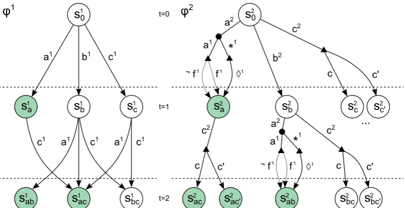
We present a two-agent example problem in which both agents have actions a, bandc, but every ac-tion can be performed only once within a 2 step horizon. Acac-tionc2 of agent 2is (for ease of exposi-tion) the only stochastic action with outcomescandc0, and corresponding probabilities0.75and0.25. There is only one interaction, between actions a1 and a2, and the reward depends on feature f1 of agent1 being set fromf1?tof1 or¬f1. Thus we have one interaction reward function with rewards

R1,2(f1?,{a1, a2}, f1)andR1,2(f1?,{a1, a2},¬f1), and local rewardsR1andR2. Without specifying actual rewards, we demonstrate the CRGs and CoRe.

Figure 2 illustrates the two CRGs. On the left is the CRGφ1of agent1with only its local rewardR1, while the CRG of agent 2 includes both the reward interaction functionR1,2 and its local rewardR2. Notice that only when sequences start with actiona2additional arcs are included in CRGφ2to account for reward interactions. The sequence starting with a2 is followed by an after-state node with two arcs: one for agent 1 performing a1 and one for its other actions, ∗1 _{= {b}1_{, c}1_{}. The interaction}

reward depends on what featuref1is (stochastically) set to, thus the influence arcsf1and¬f1are now required. As the interaction reward only occurs when{a1, a2}is executed, the fully-specified after-state node aftera2 and∗1 _{(the triangle below it) has a no-influence arc}1_{. All other transitions are reward}

independent and captured by local transitions(s1₀, b1, s1_b)and(s1₀, c1, s1_c). Locally reward independent states are highlighted green and from each of these states only the optimal action transition is kept in the CRG, e.g. only action arcc1is included froms1_a. This action was determined optimal from the local state by single-agent optimal policy search, and thus no arcs for other actions (hereb1) are necessary.

Consider for example the state s1

a ofφ1, in which actiona1 has been taken in the first time step.

From this state onward, the reward interaction between actiona1 anda2 will no longer take place and therefore agent1is locally independent. Consequentially, we can remove either the branch for actionb1

orc1_{based on which action maximises the expected value. In addition, this action will cause both agents}

to become independent from each other because of the single dependency function between them.

re-Figure 2: The CRGs of the two agents. We omit the branches fora2andb2 from statess2_c ands2_c0. The

highlighted states are locally reward independent (reward arcs are omitted).

wards. The execution sequenceθh that is evaluated is highlighted in thick red. This sequence starts

with non-dependent actions{b1, b2}, resulting in joint statesb,b (ignore the bounds in blue for now).

The execution sequence at t = 1 is thus θ1 = [s0,{b1, b2}, sb,b]. In the CRGs the corresponding

transitions to states s1_b and s2_b are shown. Now for t = 1 CoRe is evaluating joint action {a1, a2}

that is reward-interacting and thus the value of state featuref1 is required to determine the transition in φ2 _{(here chosen arbitrarily as ¬f}1

x). The corresponding execution sequence (of agent 2) is

there-foreθ2₂ = [s2₀,{b1, b2}, s2_b ∪ {f1?},{a1, a2}, s_ba2 ∪ {¬f1}]If agent 1 had chosen actionc1 instead, we would traverse the branches∗1_and1_{leading to states}2

bawithout reward interactions.

Branch-and-bound is shown (in blue) for statesb,b, with the rewards labelled on transitions and their

bounds at the nodes. The bounds for joint actions{a1, a2} and{a1, c2} are[13,16]and[12.5,12.5], respectively, found by summing the CRG bounds, hence{a1, c2}can be pruned. Note that we can com-pute the expected value of{a1, c2}in the CRG, but not that of{a1, a2}. This is because agent2knows the transition probability of actionc2but it does not know what valuef1 has during CRG generation or with what probabilitya1 will be performed. Regardless, we can bound the return of actiona2 over all possible feature values, stored inφ2, and they can be updated as the probabilities become known during policy search.

Conditional reward independence occurs in the green states of the policy search tree. After joint action{b1, a2}, the agents will no longer interact (a2 is completed and will not be available anymore) and thus the problem is decoupled. From state sb,a CoRe finds optimal policies π1∗(s1b) and π

∗

2(s2a)

and combines them into the optimal joint policyπ∗(sb,a) = hπ1∗(s1b), π

∗

2(s2a)ifor the planning problem

remaining from independent statesb,a.

6

Evaluation

In our experiments we find optimal policies for the maintenance planning problem(MPP, see the in-troduction) that minimise the (time-dependent) maintenance costs and economic losses due to traffic hindrance. In this problem agents represent contractors that participate in a mechanism and thus it is essential that the planning is done optimally.

Figure 3: Example of policy evaluation. The left graph shows (a part of) the policy search tree with joint states and joint actions, and the right graph the CRGs per agent. One possible execution sequenceθhis

highlighted in thick red.

Here we only briefly outline the problem. Agents maintain a state with start and end times of their maintenance tasks. Each of these tasks can be performed only once and agents can perform exactly one task at a time (or do nothing). The individual rewards are given by maintenance costs that are task and time dependent, while interaction rewards model network hindrance due to concurrent maintenance. Maintenance costs are task and time dependent, while interaction rewards model network hindrance due to concurrent maintenance. In this domain we conduct three experiments with CoRe to study 1) the expected value when solving centrally versus decentralised methods, 2) the impact on the number of joint actions evaluated and 3) the scalability in terms of agents.

First, we compare with a decentralised baseline by treating the problem as a (transition and obser-vation independent) Dec-MDP [Becker et al., 2003] in which agents can only observe their local state. Although the (TI-)Dec-MDP model is fundamentally different from the TI-MMDP – in the latter deci-sions are coordinated onjoint(i.e., global) observations – the advances in Dec-MDP solution methods [Dibangoye et al., 2013] may be useful for TI-MMDP problems if they can deliver sufficient quality policies. That is, since they assume less information available, the value of Dec-MDP policies willat bestequal that of their MMDP counterparts, but in practice the expected value obtained from following a decentralised policy may be lower. We investigate if this is the case in our first experiment, which com-pares the expected value of optimal MMDP policies found by CoRe with optimal Dec-MDP policies, as found by the GMAA-ICE* algorithm [Oliehoek et al., 2013a].

For this experiment we use two benchmark sets: rand[h], 3 sets of 1000 random two-agent prob-lems with horizonsh ∈ [3,4,5], andcoordint, a set of 1000 coordination-intensive instances. The latter set contains tightly-coupled agents with dependencies constructed in such a way that maintenance delays inevitably lead to hindrance unless agents coordinate their decisions when such a delay becomes known, which is ar the first time step after starting the maintenance task. Figure 4a shows the ratio

0.2 0.3 0.4 0.5 0.6 0.7 0.8 0.9 1

rand3 rand4 rand5 coordint

Dec-MDP / MMDP

(a)Vπ∗

DEC/Vπ ∗ MMDP

101 102 103 104

105 106

107

# Evaluations

Instance

(b) # joint actions evaluated

0 20 40 60 80 100

5.0 6.0 7.0 8.0 9.0 10.0

% Solved

Horizon length

(c) Perc. instances solved

10-1 100 101 102 103

Runtime (s)

Instance

(d) runtimes

0 20 40 60 80 100

2.0 3.0 4.0 5.0 6.0 7.0 8.0 9.0 10.0

% Solved

Number of agents

(e) Perc. instances solved

In our remaining experiments we used a random test setmppwith 2, 3 and 4-agent problems (400 each) with 3 maintenance tasks, horizons 5 to 10, random delay probabilities and binary reward in-teractions. We compare CoRe against several other algorithms to investigate the performance of the algorithm. The current state-of-the-art approach to solve MPP, presented in [Scharpff et al., 2013], uses the value iteration algorithm SPUDD [Hoey et al., 1999] and solves an efficient MDP encoding of the problem. SPUDD uses algebraic decision diagrams to compactly represent all rewards and is in this sense somewhat similar to our work, however it does not implicitly partition and decouple rewards. Besides the SPUDD solver we included a dynamic programming algorithm (DP) that uses a depth-first approach to maximise the Bellman equation of Equation 2. In addition to basic value iteration we im-plemented some domain knowledge in this algorithm to quickly identify and prune sub-optimal and infeasible branches during evaluation. Finally, to analyse the impact that branch-and-bound can have in a task-based planning domain such as MPP we added also a CRG-enabled policy search algorithm (CRG-PS), a variant of our CoRe algorithm that uses CRGs but not branch-and-bound pruning.

Using these algorithms, we first study the impact of using CRGs on the number of joint actions that need to be evaluated. SPUDD is not considered in this experiment because because it does not report this information. Figure 4b shows the search space size reduction by CRGs in this domain. Our CRG-enabled algorithm (CRG-PS, blue) approximately decimates the number of evaluated joint actions compared to the DP method (green). Furthermore, when value bounds are used (CoRe, red), this number is reduced even more, although its effect varies per instance.

Having observed the policy search space reduction that CoRe can achieved, we are interested in the scalability of the algorithm in terms of number of agents and planning horizon. Figure 4c shows the percentage of problems from thempptest set that are solved within 30 minutes per method (all two-agent instances were solved and hence omitted). CoRe solves more instances than SPUDD (black) of the 3 agent problems (cross marks), and only CRG-PS and CoRe solve 4-agent instances. This is because CRGs successfully exploit the conditional action independence that decouples the agentsfor most of the planning decisions. Only when reward interactions may occur actions are coordinated, whereas SPUDD always coordinates every joint decision. Notice also that the use of branch-and-bound enables CoRe to solve more instances, compared to the CRG-enabled policy search.

Next we investigate the runtime that was required by CoRe versus that by the current best known method based on SPUDD. As CoRe achieves a greater coverage than SPUDD, we compare runtimes only for instances successfully solved by the latter (Figure 4d). We order the instances on their SPUDD runtime (causing the apparent dispersion in CoRe runtimes) and plot runtimes of both. Note that as a result the horizontal axis is not informative, it is the vertical axis plotting the runtime that we are interested in. CoRe solves almost all instances faster than SPUDD, both with 2 and 3 agents, and has a greater solving coverage: CoRe failed to solve 3.4% of the instances solved by SPUDD whereas SPUDD failed 63.9% of the instances that CoRe solved.

Finally, to study the agent-scalability of CoRe, we generated a test set pyra with a pyramid-like reward interaction structure: every first action of thek-th agent depends on the first action of agent2kand agent2k+1. Figure 4e shows the percentage of solved instances from thepyratest for various problem horizons. Whereas previous state-of-the-art solved instances up to only 5 agents, CoRe successfully solved about a quarter of the 10 agent problems (h = 4) and overall solves many of the previously unsolvable instances.

7

Conclusions and Future Work

(CoRe) that uses reward bounds based on CRGs to reduce the search space size, shown to be by orders of magnitude in the maintenance planning domain. This enables CoRe to overall decrease the runtime required compared to the previously best approach and solve instances previously deemed unsolvable. The reduction in search space follows from three key insights: 1) when interactions are sparse, the num-ber of unique returns per agent is relatively small and can be stored efficiently, 2) we can use CRGs to maintain bounds on the return, and thus the expected value, and use this to guide our search, and 3) in the presence of conditional reward independence, i.e. the absence of further reward interactions, we can decouple agents during policy search.

Our experiments show that the impact of reduction is by orders of magnitude in the maintenance planning domain. This enables CoRe to solve instances that were previously deemed unsolvable. In addition, to scaling to larger instances, CoRe almost always produces solutions faster than the previously best approach. Moreover, CoRe is able to scale up to 10-agent instances when the reward structure exhibits a high level of conditional reward independence, whereas previous methods did not scale beyond 5 agents. Finally, our experiments also illustrate that using a decentralised MDP approach, a line of research that has seen many scalable approaches in terms of agents and reward structures, leads to suboptimal expected policy values.

Here only optimal solutions are considered, but CRGs can be combined with approximation in sev-eral ways. First, the reward structure of the problem itself may be approximated. For instance, the reward-function approximation of [Koller and Parr, 1999] can be applied to increase reward sparsity, or CRG paths with relatively small reward differences may be grouped, trading off a (bounded) reward loss for compactness. Secondly, the CRG bounds directly lead to a bounded-approximation variant of CoRe, usable in for instance the approximate multi-objective method of [Roijers et al., 2014]. Lastly, the CRG structure can be implemented in any (approximate) TI-MMDP algorithm or, vice versa, any existing approximation scheme for MMDP that preserves TI can be used within CoRe.

Although we focused on transition-independent MMDPs, CRGs may be interesting for general MMDPs when transition dependencies are sparse. This would require including dependent-state tran-sitions in the CRGs similar to reward-interaction paths and is considered to be future work. Another interesting avenue is to exploit conditional reward independence during joint action generation.

Acknowledgements

This research is supported by the NWO DTC-NCAP (#612.001.109), Next Generation Infrastructures, Almende BV and NWO VENI (#639.021.336) projects.

Appendix: Proof of Theorem 2

In this appendix, we prove the correctness of the CoRe algorithm (Theorem 2).

We define several notational shorthands for convenience. For two (sub)sets of agentsA, B ⊆ N,

Re

AB ⊆ Ris the set of all rewards for whichA∩B∩e =6 ∅. ReA6B ⊆ Ris the set of rewards such

thatA∩e 6= ∅ and B ∩e = ∅. Observe that the individual rewards for all agentsa ∈ A are thus contained within Re

A6B (and similarly all rewards Rb are included inRe6AB). Furthermore, two agent

setsAandB are conditionally reward independent, denotedCRI(A, B, θt), as result of historyθt iff ∀a∈A, b∈B:CRI(a, b, θt). Finally,τe = ({sj}j∈e,{~aj}j∈e,{sˆj}j∈e)denotes a transition local to

agentseand a global transition, i.e.e=N, is denoted byτ.

Lemma A.1. Given an execution historyθt= [s0, ~a0, . . . , su, . . . , st]up to timetthat can be partitioned

into two histories,θu = [s0, . . . , su]andθu0 = [s_u, . . . , s_t], and a disjoint partitioning of agents N =

The returnZ(θt)(as defined in Equation 3) can be decoupled as:

Z(θu) + k X

i=1

ZNi(θ

Ni

u0) (A.13)

whereθNi

u0 is the execution history only containing the states and actions of the agents in the setNi ⊆N,

starting from timeu.

Proof. Recall from Definition 5 that two agents i, j ∈ N areCRI iff ∀Re ∈ R s.t. {i, j} ⊆ e:

Ph

x=tRe(sx, ~ax, sx+1) = 0for every pair of statesst, st+1and all joint actions~at, given execution

his-toryθt. Moreover, recall that the MMDP rewardsRw.l.o.g. are structured asR(τ) =PRe_∈RRe(τe). Let AandB be disjoint subsets of agents such thatA∪B = N and let the reward functions be accordingly partitioned as disjoint sets:R=Re

A6B∪Re6AB∪ReAB. Now assume that for a given execution

historyθt=θu∪θu0we haveCRI(A, B, θ_u). From the states_uresulting from the execution historyθ_u,

all future rewards can only be local with respect to subsetsAandBbecause every rewardR_ABe must be zero by definition of CRI. Therefore we can rewrite the (future) global rewardR(τ)of every possible transitionτ (in every possibleθNi

u0) as:

X

Re_∈Re

Re(τ) =Re_A6B(τA) +R_ABe₆ (τB) +Re_AB(τAB) (A.14)

= X

Re_∈Re A6B

Re(τA) + X

Re_∈Re

6

AB

Re(τB) (A.15)

where the transition decoupling is possible due to transitional independence. Remember that we can write the returns for an execution historyθh as (Eq. 3)

Z(θt) = t−1 X

x=0 X

Re_∈R

Re(τ_θ,xe ) (A.16)

in whichτ_θe denotes the transition in the execution historyθtlocal to agents e. Then, for two disjoint

agent subsetsA∪B =N that haveCRI(A, B, θu)as a result ofθu:

Z(θt) =Z(θu) +Z(θu0) (A.17)

=Z(θu) + t−1 X

x=u

Re_A6B(τ_θ,xA ) +Re_6AB(τ_θ,xB ) (A.18)

=Z(θu) + t−1 X

x=u Re

A6B(τθ,xA) + t−1 X

x=u Re

6

AB(τθ,xB) (A.19)

=Z(θu) +ZA(θuA0) +Z_B(θB_u0) (A.20)

As a consequence, we can decouple the computation of returns for agent setsAandBfrom timeu. For now we have only considered two agent setsAandB, however we can apply this decoupling recursively, in order to obtain an arbitrary disjoint partitioning of agents such thatN1∪N2∪. . .∪Nk =N

and∀Na, Nb ∈ N : CRI(Na, Nb, θu). That is, without loss of generality, we choose A = Na and

B =N2∪. . .∪Nkand decouple the return asZ(θu) +ZA(θ_uA0) +ZB(θ_uB0). We now observe that we can

rewriteZB itself asZN2(θ

N2

u0 ) +Z_B\N2(θ

B\N2

u0 )by following the same steps, because both sets again

satisfy conditional reward independence. By continuing this process we obtain Equation A.13.

As a result of Lemma A.1, Equation 4 and transitional independence we can now also decou-ple the policy values of two sets of agents, Na and Na, from time u onwards, when it holds that

Corollary A.1. When at a timestep u, we have observed θu and there is a disjoint partitioning of

agentsN =N1∪N2 ∪. . .∪Nksuch that for every pairNa, Nb ∈ N it holds thatCRI(Na, Nb, θu)

whena6=b, the value of a given policyπ,V(st)can be decoupled as:

Vπ(st) = k X

i=1

V_Nπ_i(sNi

t ) (A.21)

Proof. Starting from Equation 4, we first observe that the returnZ(θu0) from timestep u onwards is

equal to Pk

i=1ZNi(θ

Ni

u0) (Lemma A.1) and that, because of transition independence, each set Ni of

agents has independent probability distributions over future execution historiesθu0. Thus we have the

following equalities:

V(st) = X

θu0|π,θt

P r(θu0)Z(θ_u0) (A.22)

= X

θ_u0|π,θt

P r(θu0)

k X

i=1

ZNi(θ

Ni

u0 ) =

X

θ_u0|π,θt

k X

i=1

P r(θu0)Z_N

i(θ

Ni

u0 ) (A.23)

=

k X

i=1 X

θ_u0|π,θt

P r(θu0)Z_N

i(θ

Ni

u0 ) =

k X

i=1 X

θNi

u0|π,θt

P r(θNi

u0 )ZNi(θ

Ni

u0) (A.24)

=

k X

i=1

V_Nπ_i(sNi

t ) (A.25)

Lemma A.2. The bounding heuristicsL(se_t)andU(se_t)used to prune during branch-and-bound search are admissible with respect to the expected valueV(se_t)of statese_tfor agentse⊆N at timet.

Proof. We proof the admissibility of the bounding heuristics by induction. For sake of brevity, we only show the upper bound proof, but the proof for the lower bound can be written down accordingly. Recall thatR=S

i∈NRiis the disjoint partitioning of reward functions over the CRGs.

First, consider the very last timestep,h−1, for which there is no future reward, i.e.,

V(sh−1) = max ~a

X

sh∈S

T(τh−1)R(τh−1) = max ~a

X

sh∈S

T(τh−1) X

i∈N

Ri(τhe−1) (A.26)

≤max

~a maxsh∈S

X

i∈N

Ri(τhe−1) (A.27)

≤X

i∈N

max

τe

h−1∈φi(sih−1)

Ri(τhe−1) (A.28)

=X

i∈N

U(si_h−1) (A.29)

Then, we show that if for a next stage t+ 1we have a valid upper bound, the value for a state st is

also upper bounded byP

V(sh−1), the upper bound is admissible for all stages beforeh−1:

V(st) = max ~a

X

se t+1∈S

T(τt) (R(τt) +V(st+1)) (A.30)

= max

~ae

X

st+1∈S

T(τt) V(st+1) + X

i∈N

Ri(τte) !

(A.31)

≤max

~ae

X

st+1∈S

T(τt) X

i∈N

R_i(τ_te) +U(si_t+1)

(A.32)

≤X

i∈N

max

τte∈φi(sit)

Ri(τte) +U(sit+1)

(A.33)

=X

i∈N

U(si_t) (A.34)

From the bounds on the state-values,

L(st) = X

i∈N

L(si_t)≤V(st)≤ X

i∈N

U(si_t) =U(st),

we can also distill admissible bounds on state-action values,Q(st, ~a). Taking the standard MDP

defini-tion forQ(st, ~a),

Q(st, ~a) = X

ˆ st+1∈S

T(st, ~a,ˆst+1) (R(st, ~a,ˆst+1) +V(st+1)),

we replaceV(st+1)by the corresponding lower or upper bounds:

B(st, ~a) = X

ˆ st+1∈S

T(st, ~a,sˆt+1) (R(st, ~a,ˆst+1) +B(st+1)).

UsingB(st, ~a), CoRe can exclude a joint action~aafter execution historyθtfrom consideration when

there is another joint action ~a0 for which U(st, ~a) ≤ L(st, ~a0), as is standard in branch-and-bound

algorithms.

Concluding the proof of Theorem 2. As a direct consequence of Corollary A.1 agents can be decoupled during policy search without losing optimality. Moreover, Lemma A.2 shows that both the upper and lower bounds are admissible heuristic functions with respect to the expected policy value from a given state. In the main loop, the CoRe algorithm recursively expands and evaluates all possible extensions to the current execution path, except for those starting with actions that lead to a lower upper bound than another action’s lower bound.

As the policy search considers all possible execution histories, excluding pruned, non-optimal ones, the search will eventually return the optimal policy valueV∗, and corresponding policy, thus proving Theorem 2.

References

[Bakker et al., 2010] Bakker, B., Whiteson, S., Kester, L., and Groen, F. (2010). Traffic Light Control by Multiagent Reinforcement Learning Systems, chapter Interactive Collaborative In-formation Systems, pages 475–510. Studies in Computational Intelligence, Springer.

[Becker et al., 2004] Becker, R., Zilberstein, S., and Lesser, V. (2004). Decentralized Markov decision processes with event-driven interac-tions. In Proceedings of the Int. Conf. on Autonomous Agents and Multiagent Systems, pages 302–309.

[Becker et al., 2003] Becker, R., Zilberstein, S., Lesser, V., and Goldman, C. V. (2003). Transition-independent decentralized Markov decision processes. In Proceedings of the Int. Conf. on Autonomous Agents and Multiagent Systems, pages 41–48.

[Boutilier, 1996] Boutilier, C. (1996). Planning, learning and coordination in multiagent deci-sion processes. In Proceedings of the Int. Conf. on Theoretical Aspects of Rationality and Knowledge.

[Cavallo et al., 2006] Cavallo, R., Parkes, D. C., and Singh, S. (2006). Optimal coordinated plan-ning amongst self-interested agents with private state. InProceedings of Uncertainty in Artificial Intelligence.

[De Hauwere et al., 2012] De Hauwere, Y.-M., Vrancx, P., and Now´e, A. (2012). Solving sparse delayed coordination problems in multi-agent reinforcement learning. InAdaptive and Learning Agents, pages 114–133. Springer.

[Dibangoye et al., 2013] Dibangoye, J. S., Am-ato, C., Doniec, A., and Charpillet, F. (2013). Producing efficient error-bounded solutions for transition independent decentralized MDPs. In Proceedings of the Int. Conf. on Autonomous Agents and Multiagent Systems.

[Guestrin et al., 2002a] Guestrin, C., Koller, D., and Parr, R. (2002a). Multiagent planning with factored MDPs. In Advances in Neural Infor-mation Processing Systems 14. MIT Press.

[Guestrin et al., 2002b] Guestrin, C., Venkatara-man, S., and Koller, D. (2002b). Context-specific multiagent coordination and planning with factored MDPs. In Proceedings of the Eighteenth National Conference on Artificial Intelligence, pages 253–259.

[Hoey et al., 1999] Hoey, J., St-Aubin, R., Hu, A., and Boutilier, C. (1999). SPUDD: Stochastic planning using decision diagrams. Proceedings of Uncertainty in Artificial Intelligence.

[Kok and Vlassis, 2004] Kok, J. R. and Vlassis, N. (2004). Sparse cooperative Q-learning. In Pro-ceedings of the Int. Conf. on Machine Learning, pages 481–488.

[Koller and Parr, 1999] Koller, D. and Parr, R. (1999). Computing factored value functions for policies in structured MDPs. InProceedings of the International Joint Conference on Artificial Intelligence, pages 1332–1339.

[Melo and Veloso, 2009] Melo, F. S. and Veloso, M. (2009). Learning of coordination: Ex-ploiting sparse interactions in multiagent sys-tems. In Proceedings of The 8th Int. Conf. on Autonomous Agents and Multiagent Systems-Volume 2, pages 773–780. International Foun-dation for Autonomous Agents and Multiagent Systems.

[Melo and Veloso, 2011] Melo, F. S. and Veloso, M. (2011). Decentralized MDPs with sparse interactions. Artificial Intelligence, 175(11):1757–1789.

[Messias et al., 2013] Messias, J. V., Spaan, M. T. J., and Lima, P. U. (2013). GSMDPs for multi-robot sequential decision-making. In Pro-ceedings of the Twenty-Seventh AAAI Confer-ence on Artificial IntelligConfer-ence, pages 1408– 1414.

[Mostafa and Lesser, 2009] Mostafa, H. and Lesser, V. (2009). Offline planning for commu-nication by exploiting structured interactions in decentralized MDPs. In Proceedings of the International Joint Conference on Web Intelligence and Intelligent Agent Technologies, volume 2, pages 193–200.

[Nair et al., 2005] Nair, R., Varakantham, P., Tambe, M., and Yokoo, M. (2005). Networked distributed POMDPs: A synthesis of distributed constraint optimization and POMDPs. Proceed-ings of the Twentieth National Conference on Artificial Intelligence.

[Oliehoek et al., 2013a] Oliehoek, F. A., Spaan, M. T. J., Amato, C., and Whiteson, S. (2013a). Incremental clustering and expan-sion for faster optimal planning in decentralized POMDPs. Journal of Artificial Intelligence Re-search, 46:449–509.

[Oliehoek et al., 2008] Oliehoek, F. A., Spaan, M. T. J., Whiteson, S., and Vlassis, N. (2008). Ex-ploiting locality of interaction in factored Dec-POMDPs. In Proceedings of the Int. Conf. on Autonomous Agents and Multiagent Systems, pages 517–524.

[Oliehoek et al., 2015] Oliehoek, F. A., Spaan, M. T. J., and Witwicki, S. J. (2015). Factored upper bounds for multiagent planning problems under uncertainty with non-factored value functions. In Proc. of International Joint Conference on Artificial Intelligence, pages 1645–1651.

[Oliehoek et al., 2013b] Oliehoek, F. A., White-son, S., and Spaan, M. T. J. (2013b). Approxi-mate solutions for factored Dec-POMDPs with many agents. In Proceedings of the Int. Conf. on Autonomous Agents and Multiagent Systems, pages 563–570.

[Parr, 1998] Parr, R. (1998). Flexible decomposi-tion algorithms for weakly coupled Markov de-cision problems. InProceedings of Uncertainty in Artificial Intelligence, pages 422–430. Mor-gan Kaufmann Publishers Inc.

[Puterman, 2014] Puterman, M. L. (2014). Markov decision processes: discrete stochastic dynamic programming. John Wiley & Sons.

[Roijers et al., 2014] Roijers, D. M., Scharpff, J., Spaan, M. T. J., Oliehoek, F. A., De Weerdt, M., and Whiteson, S. (2014). Bounded approx-imations for linear multi-objective planning un-der uncertainty. InProceedings of the Int. Conf. on Automated Planning and Scheduling, pages 262–270.

[Scharpff et al., 2013] Scharpff, J., Spaan, M. T. J., de Weerdt, M., and Volker, L. (2013). Planning under uncertainty for coordinating in-frastructural maintenance. InProceedings of the Int. Conf. on Automated Planning and Schedul-ing, pages 425–433.

[Spaan et al., 2006] Spaan, M. T. J., Gordon, G. J., and Vlassis, N. (2006). Decentralized planning under uncertainty for teams of communicating agents. InProceedings of the Int. Conf. on Au-tonomous Agents and Multiagent Systems.

[Varakantham et al., 2007] Varakantham, P., Marecki, J., Yabu, Y., Tambe, M., and Yokoo, M. (2007). Letting loose a SPIDER on a network of POMDPs: Generating quality guaranteed policies. InProceedings of the Int. Conf. on Autonomous Agents and Multiagent Systems.