Fast Transforms Algorithms, Analyses, Applications tqw darksiderg pdf

(1)

(2)

(3)

FAST TRANSFORMS

Algorithms, Analyses, Applications

Douglas F.

Elliott

Electronics Research Center Rockwell International Anaheim, California

K. Ramamohan Rao

Department of Electrical Engineering The University of Texas at Arlington Arlington, Texas

A C A D E M I C P R E S S , I N C . (Harcourt Brace Jovanovich, Publishers)

(4)

N O PART O F THIS P U B L I C A T I O N M A Y B E REPRODUCED OR T R A N S M I T T E D I N A N Y F O R M OR B Y A N Y M E A N S , E L E C T R O N I C OR M E C H A N I C A L , I N C L U D I N G PHOTOCOPY, RECORDING, OR A N Y I N F O R M A T I O N STORAGE AND RETRIEVAL S Y S T E M , W I T H O U T P E R M I S S I O N I N W R I T I N G F R O M THE PUBLISHER.

A C A D E M I C P R E S S , I N C .

Orlando, Florida 32887

United Kingdom Edition published by

A C A D E M I C P R E S S , I N C . ( L O N D O N ) L T D .

24/28 Oval Road, London N W 1 7 D X

Library of Congress Cataloging in Publication Data

Elliott, Douglas F.

Fast transforms: algorithms, analyses, applications.

Includes bibliographical references and index. 1. Fourier transformations—Data processing.

2. Algorithms. I. Rao, K. Ramamohan (Kamisetty Ramamohan) II. Title. III. Series

QA403.5.E4 515.7'23 79-8852 ISBN 0-12-237080-5 AACR2

AMS (MOS) 1 9 8 0 Subject Classifications: 6 8 C 2 5 , 4 2 C 2 0 , 6 8 C 0 5 , 4 2 C 1 0

P R I N T E D I N T H E U N I T E D STATES O F AMERICA

(5)

(6)

(7)

PREFACE

Fast transforms are playing an increasingly important role in applied engi-neering practices. N o t only do they provide spectral analysis in speech, sonar, radar, and vibration detection, but also they provide bandwidth re-duction in video transmission and signal filtering. F a s t transforms are used directly to filter signals in the frequency domain and indirectly to design digital filters for time domain processing. They are also used for convolution evaluation and signal decomposition. Perhaps the reader can anticipate other applications, and as time passes the list of applications will doubtlessly grow.

. At the present time to the authors' knowledge there is no single b o o k that discusses the m a n y fast transforms and their uses. The p u r p o s e of this book is to provide a single source that covers fast transform algorithms, analyses, and applications. It is the result of collaboration by an author in the aero-space industry with another in the university community. The authors hope that the collaboration has resulted in a suitable mix of theoretical develop-ment and practical uses of fast transforms.

This book has grown from notes used by the authors to instruct fast transform classes. One class was sponsored by the Training D e p a r t m e n t of Rockwell International, and another was sponsored by the Department of Electrical Engineering of The University of Texas at Arlington. Some of the material was also used in a short course sponsored by the University of Southern California. The authors are indebted to their students for motivat-ing the writmotivat-ing of this b o o k and for suggestions to improve it.

(14)

The long list of references at the end of the book attests to the volume of literature on fast transforms and related digital signal processing. Since it is impractical to cover all of the information available, the authors have tried to list as many relevant references as possible under some of the topics dis-cussed only briefly. The authors hope this will serve as a guide to those seeking additional material.

(15)

A C K N O W L E D G M E N T S

It is a pleasure to acknowledge helpful discussions with our colleagues who contributed to our understanding of fast transforms. In particular, fruit-ful discussions w e r e held with T h o m a s A. Becker, William S. Burdic, Tien-Lin Chang, Robert J. Doyle, Lloyd O. K r a u s e , David A. Orton, David L . Hench, Stanley A. White, and L e e S. Young of Rockwell International; Fredric J. Harris of San Diego State University and the N a v a l Ocean Sys-tems Center; I. Luis Ayala of Vitro T e c , M o n t e r r e y , M e x i c o ; and Patrick Yip of McMaster University. It is also a pleasure to acknowledge support from Thomas A. Becker, M a u r o J. Dentino, J. David Hirstein, T h o m a s H . Moore, Visvaldis A. Vitols, and Stanley A. White of Rockwell International and Floyd L . Cash, Charles W. Jiles, John W. R o u s e , Jr., and A n d r e w E . Salis of The University of Texas at Arlington.

Portions of the manuscript were reviewed by a n u m b e r of people w h o pointed out corrections or suggested clarifications. T h e s e people include Thomas A. Becker, William S. Burdic, Tien-Lin Chang, Paul J. Cuenin, David L. H e n c h , Lloyd O. K r a u s e , James B . L a r s o n , L e s t e r Mintzer, Thomas H . M o o r e , David A. Orton, Ralph E . Smith, Jeffrey P. Strauss, and Stanley A. White of Rockwell International; H e n r y J. N u s s b a u m e r of the Ecole Polytechnique Federate de L a u s a n n e ; R a m e s h C. Agarwal of the Indian Institute of Technology; Minsoo Suk of the K o r e a A d v a n c e d Institute of Science; Patrick Yip of M c M a s t e r University; Richard W. Hamming of the Naval Postgraduate School; G. Clifford Carter and Albert H . Nuttall of the Naval U n d e r w a t e r Systems Center; C. Sidney Burrus of Rice Univer-sity; Fredric J. Harris of San Diego State University and the Naval Ocean Systems Center; Samuel D . Stearns of Sandia Laboratories; Philip A. Hal-lenborg of N o r t h r u p Corporation; I. Luis Ayala of Vitro T e c ; George Szentirmai of C G I S , Palo Alto, California; and Roger Lighty of the Jet Pro-pulsion Laboratory.

The authors wish to thank several hardworking people w h o contributed to the manuscript typing. The bulk of the manuscript was typed by M r s .

(16)

Ruth E . Flanagan, M r s . Verna E . J o n e s , and M r s . Azalee Tatum. T h e authors especially appreciate their patience and willingness to help far be-yond the call of duty.

(17)

L I S T

OF

A C R O N Y M S

A D C Analog-to-digital converter F O M Figure of merit

A G C Automatic gain control F W T Fast Walsh transform

B C M Block circulant matrix G C B C Gray code to binary conversion

B I F O R E Binary Fourier representation G C D Greatest c o m m o n divisor

B P F Bandpass filter G T Generalized discrete transform

BR Bit reversal ( G T )r rth-order generalized discrete

B R O Bit-reversed order transform

CBT Complex B I F O R E transform H H T H a d a m a r d - H a a r transform

C C P Circular convolution property (HHT),. rth-order H a d a m a r d - H a a r

C F N T Complex F e r m a t number transform

transform H T H a a r transform

C H T Complex H a a r transform I D C T Inverse discrete cosine transform

C M N T Complex Mersenne number I D F T Inverse discrete Fourier transform

transform I F Intermediate frequency

C M P Y Complex multiplications I F F T Inverse fast Fourier transform

C N T T Complex number theoretic I F N T Inverse F e r m a t n u m b e r transform

transform I G T Inverse generalized transform

C P F N T Complex pseudo-Fermat number ( I G T )r rth-order inverse generalized

transform transform

C P M N T Complex pseudo-Mersenne num- I I R Infinite impulse response

ber transform I M N T Inverse Mersenne number

C R T Chinese remainder theorem transform

D A C Digital-to-analog converter K L T K a r h u n e n - L o e v e transform

D C T Discrete cosine transform L P F Low pass filter

D D T Discrete D transform lsb Least significant bit

D F T Discrete Fourier transform lsd Least significant digit

D I F Decimation in frequency M B T Modified B I F O R E transform

D I T Decimation in time M C B T Modified complex B I F O R E

D M Dyadic matrix transform

D S T Discrete sine transform M G T Modified generalized transform

E N B R Effective noise bandwidth ratio ( M G T )r rth-order modified generalized

dis-E N B W Equivalent noise bandwidth crete transform

E P E Energy packing efficiency M I R Mixed radix integer representation

F D C T Fast discrete cosine transform M N T Mersenne n u m b e r transform

F F T Fast Fourier transform M P Y Multiplications

F G T Fast generalized transform msb Most significant bit

F I R Finite impulse response msd Most significant digit

F N T Fermat number transform mse Mean-square error

(18)

M W H T Modified W a l s h - H a d a m a r d S H T S l a n t - H a a r transform

transform (SHT), rth-order slant-Haar transform

( M W H T )h H a d a m a r d ordered modified SIR Second integer representation

( M W H T )h

W a l s h - H a d a m a r d transform S N R Signal-to-noise ratio

N P S D Noise power spectral density ST Slant transform.

N T T N u m b e r theoretic transform W F T A Winograd Fourier transform

P S D Power spectral density algorithm

R F Radio frequency W H T W a l s h - H a d a m a r d transform

R H T Rationalized H a a r transform ( W H T )C S Cal-sal ordered W a l s h - H a d a m a r d

R H H T Rationalized H a d a m a r d - H a a r transform

transform ( W H T )h H a d a m a r d ordered W a l s h

-( R H H T )r rth-order rationalized H a d a m a r d - H a d a m a r d transform

( R H H T )r

H a a r transform ( W H T )p Paley ordered W a l s h - H a d a m a r d

R M F F T Reduced multiplications fast transform

Fourier transform ( W H T )W Walsh ordered W a l s h - H a d a m a r d

R M S R o o t mean square transform

R N S Residue number system zps Zero crossings per second

(19)

N O T A T I O N

Symbol A, B,... A® B AT A'1 D(f) D(f) D'(f) D'(f)

D F T [ j c ( w ) ]

\Pr{L)-\ E

Ft

iHmh{Ly]

Meaning

Matrices are designated by capital letters

The Kronecker product of A

and B (see Appendix)

The transpose of matrix A

The inverse of matrix A

D C T matrix of size ( 2L_{x 2}L₎

Periodic D F T filter frequency

response, which for P = 1 s

is given by

sin(7t/)

N/JNsm(nf/N)

Periodic frequency response of D F T with weighted input (windowed output) Nonperiodic D F T filter

fre-quency response which for

P = 1 s is given by

exp[-77i/(l - 1/AO] [sin(7r/)]/(7c/)

Nonperiodic frequency re-sponse of D F T with weighted input (windowed output)

The discrete Fourier trans-form of the sequence

MO), x ( l ) , ...,x(N- 1)}

7'th matrix factor of [G>(L)] Expectation operator

7'th matrix factor of \_Mr(L)~\

rth Fermat number, Ft =

( 22 t

+ 1), t = 0, 1 , 2 , . . .

( G T )r matrix of size ( 2

L_{x 2}L₎

M W H T matrix of size ( 2L

x 2L

)

Symbol Meaning

[ #S( L ) ] W a l s h - H a d a m a r d matrix of

size ( 2L_{x 2}L_{) . T h e}

sub-script s can be w, h, p , or cs,

denoting Walsh,

H a d a m a r d , Paley or cal-sal ordering, respectively.

[Ha(L)] H a a r matrix of size ( 2L_{x 2}L₎

[ H hr( L ) ] rth order ( H H T )r matrix of

size ( 2L_{x 2}L₎

Im Opposite diagonal matrix,

e.g.,

~ 0 0 0 f

0 0 1 0 0 1 0 0 1 0 0 0

7^m

Columns of IN are shifted

cir-cularly to the right by m

places

7^w

Columns of IN are shifted

cir-cularly to the left by m

places

1% Columns of IN are shifted

dyadically by / places

IR Identity matrix of size (R x R)

I m [ ] T h e imaginary part of the quantity in the square brackets

IDFT[X(/c)] T h e inverse discrete Fourier

transform of the sequence

{X(0),X(l),...,X(N-l)} [K(L)] K L T matrix of size ( 2L

x 2L

)

L Integer such that N = ccL

MP Mersenne number,

MP = 2 P

— 1, where P i s a prime n u m b e r

(20)

Symbol Meaning

(MGT),. matrix of size ( 2L

x 2L

)

TV Transform dimension

N'1 _{Multiplicative inverse of the}

integer TV such that TV x TV"1

= 1 (modulo M)

P 1. Period of periodic time

function in seconds 2. I n Chapter 11, prime

number

Diagonal matrix whose diagonal elements are neg-ative integer powers of 2

( W H T )h circular

shift-invariant power spectral point

^ ( / ) /th power spectral point of (GT),

rath sequency power spectrum

Q 1. Ratio of the filter center

frequency and the filter bandwidth (Chapter 6) 2. Least significant bit value

(Chapter 7)

R e [ ] The real part of the quantity in

the square brackets

* ( D ) Rate distortion

[Rh(L)] R H T matrix of size ( 2L

x 2L

)

ST matrix of size ( 2L

x 2L

)

[S<°">(L)] Shift matrix relating X(c"° and

v

[S( c m )_(L)]

A.

Shift matrix relating X( c m )_and

V

OTL)] _{Shift matrix relating}A _X( d Z ) and

Y

[Sh,.(L)]

A.

rth order (SHT),. matrix of size ( 2L

x 2L

)

r Sampling interval

1. exp(-y'27r/TV) for F F T 2. e x p ( - 7 2 7 i / ar + 1_{) for F G T}

The element • in a matrix means — 700 so that

Shorthand notation for

matrix product WA

WB ,

where A and B are TV x TV

matrices

WE

Matrix with entry WE{k,n)

in

row k and column n, where

i?is a matrix of size (TV x TV),

E(k, n) is the entry in row k

and column n for k,

n = 0 , 1 , . . . , T V - 1

Symbol Meaning

X(f) o r XJif) Spectrum defined by t h e

Fourier (or generalized) transform of the (analog)

function x(t)

\X(f)\2

Power spectral density with units of watts per hertz

X(k) Coefficient number k, k = 0,

+ 1 , ±2, . . . , in series

expansion of periodic

function x(t)

\X(k)\2 Power spectrum for a function

with a series representation

Xc D C T of x

C F N T of x

£ ( c m ) _{Transform of}_xcm

Transform of xcm

Y

A_{c r a} C M N T of x

Xc pf C P F N T of x

Y

^ c p m C P M N T of x

x( d / ) Transform of xdl

xf F N T of x

^ h a H T of x ^ h h r ( H H T )r of x

xk K L T of x

xm M N T of x

^ m h M W H T of x

( M G T )r of x

Xpf P F N T of x

Y P M N T of x

xr (GT),. of x

^(cra) _{( G T )} r of x

c m

R H T of x

xs ST of x

kth W H T coefficient. T h e

subscript s is defined in

(SHT), of x

ZM Ring of integers modulo M

represented by the set

{ 0 , 1 , 2 , . ..,M- 1}

7C

M Ring of complex integers. If

c = a + p, where a, =

R e [ > ] a n d S- — I m[ Y ] , t h e n

c is represented in ZC

M by

a, + j3, where a, = a

m o d M and 6- = I m o d M

a^b Give variable a the value of

expression b (or replace a

by b)

aeB a is an element of the set B

a e [c, J ) c ^ a < d

combj^ The infinite series of impulse

(21)

NOTATION xxi

Symbol Meaning Symbol Meaning

f fk

I 8{t-kT) k= — oo

cube[7//?] Cubic-shaped function defined by

c u b e - = tri , — * tri

LpA I_P/2J LP/2J

deg[ ] The degree of the polynomial in the square brackets Frequency in hertz Digit in expansion of

m

where / is the least significant digit (lsd) and

m is the most significant

digit (msd)

fs = \IT is the sampling

frequency

Element of [//S(L)] in row k

and column n. The

subscript s is defined in

Transform coefficient number The decimal number obtained

by the bit reversal of the L

bit binary representation of

k

The integer defined by

hs(k,n)

J k

k-s

In

log l o g2

n

I K+i-i2 s ~l

,

1 = 0

where s = r + 2, r + 3, . . . , L,

k = 2r , 2r + 1

, . . . , ( 2r + 1

- l ) ,

and fc/s/ = 0, 1 , . . . , r + 1,

is a bit in the binary

representation of k

Logarithm to the base e

(natural logarithm) Logarithm to the base 10 Logarithm to the base 2 D a t a sequence number Integerization of frequency

given by

rad(m, t)

rect[r/P]

rep/sD*l/)]

sincC/(2) t

tr[ ] tri[f/P]

«(^-^o)

wals(/c, r)

x{n)

x{n)^X(k) x(t)

x(0

x ( O ^ W )

x o y

Integer in the set ( 0 , 1 , 2 , . . . , L - 1) mth Rademacher function Rectangular-shaped function

defined by

1, W^P/2

0, otherwise

The repetition of X(f) every fs

units as defined by the

convolution X{f) * comb^s

Seconds [sin(7c/fi)]/(7c/0

Time in seconds Trace of a matrix

Triangular-shaped function defined by

tri — = r e c t * r e c t

LPJ LP/2J LP/2J

Unit step function defined by

u(t-t0) =

0, otherwise

kih Walsh function. The

sub-script s is defined in

LHs(Lj]

Complex conjugate of x

x shifted circularly to the left

by m places

x shifted circularly to the right

by m places

x is shifted dyadically by /

places

Sampled-data value of x for

sample number n

Both x{n) and X(k) exist Time domain scalar-valued

function at time t

Time domain vector-valued

function at time t

Both x(t) and X(f) exist Sampled function

The convolution of x and y

Element by element multi-plication of the elements in

x and y, e.g., if a = x o y ,

then a(k) = x(k)y(k)

Expression for x in number

(22)

Symbol Meaning Symbol

inn

. m o d &

l\N

^ld(t-T)l=exp(-j2nfT)

Fourier transform operator

T h e remainder when a is

divided by ^ Generalized transform

operator

Fourier transform of u>(t)

6,... Script lower case letters a,

. . . and the italic letters /,

k, I, m, n, p, q, r (Chapter 5

only), K, L, M, and N

de-note integers

= 6 (modulo n) 0t{ajri) = M(#/ri), where a

and S- are either integers or

polynomials

0t{a,j&\ where a and 6 are either integers or poly-nomials

/ divides TV, i.e., the ratio N/l is

an integer and the set of such integers includes 1 and TV

Steps per second taken by the generalized transform basis functions

Weighting function applied to modify D F T filter fre-quency response

Covariance matrix of x

N u m b e r system radix or a primitive root of order TV N u m b e r of equal sectors on the unit circle in the com-plex plane with first sector starting on the positive real axis a>(t) a BAD Xj V-p a2 <M") KOI IKOII r(-)i L(-)J Meaning

Kronecker delta function with the property that

hi = 0,_1, k±l _{k = l}

Dirac delta function with the property that

*(*o) = 5{t - t0)x(t) dt

/th phase spectral point of ( G T )r

7'th eigenvalue of [ZX(LJ]

£[x]

Correlation coefficient

E[_(x - ^)2_]

The number of integers less than TV and relatively prime to TV

kth basis function 4>k(t)

eval-uated at t = nT

Magnitude of (•)

Integerize by truncation (or rounding)

Smallest integer ^ (•), e.g., [3.51 = 4, r— 2.51 = - 2 Largest integer ^ (•), e.g.,

L3.5J = 3 , L- 2 . 5 J = - 3 Signed digit addition

(23)

C H A P T E R 1

I N T R O D U C T I O N

1.0 Transform Domain Representations

Many signals can be expressed as a series that is a linear combination of orthogonal basis functions. The basis functions are precisely defined (mathe-matically) waveforms, such as sinusoids. The constant coefficients in the series expansion are computed using integral equations. Let the basis functions be specified in terms of an independent variable t and be represented as cj)k(t) for k = . . . , — 1, 0, 1, 2 , . . . . Let x(t) be the signal and X(k) be the kth coefficient. Then the signal x(t) can be decomposed in terms of the basis functions (j>k{t) as

x{t)= X XiftMt) (1.1)

If (1.1) describes x(f) for all values of t, it also describes x(t) for specific values of

t. Suppose these values are nT where T is fixed and « = ...,— 1, 0, 1, 2 , . . . . Define x(n) and cf)k(n) as x(t) and (f)k(t), respectively, evaluated at t = nT. Then

(1.1) becomes

(1.2)

Now suppose that only N of the coefficients in (1.1) are nonzero, and let those nonzero coefficients be X(0), X(l), X{2),X(N- 1). Then (1.2) reduces to

x(n) =

N

_^X{k)Un)

₍₁

_-3)

Let <P be the matrix defined by

<P =

4>o(0)

0o(l)

</>i(0)

<Mi)

4>N-i(0)

\_<j>o(N-l) h(N-l) ••• 0N_t( i V - l ) J

(1.4)

(24)

and let X be the vector defined by

X = [X(0), X ( l )3 X(2), , . . , X(7V - 1 ) ]

T₍₁_.5)

where the superscript T denotes the transpose. Then (1.3) can be written as a matrix-vector equation that specifies N variables x(0), x ( l ) , . . , , x(N - 1):

x = <f>X (1.6)

x = [x(0), x(l), x(2), ...,x(N- 1 ) ]T_(1.7)

The TV coefficients in (1.5) scale the values of <P in (1.6) and result in a complete description of x. Since the basis function values in <P are well defined and since (1.6) is a matrix-vector equation (or transformation), the components of X constitute a transform domain representation of x .

The transform domain representation of x is especially useful in signal processing using digital computers. If x(0), x ( l ) , x( 2 ) , . . . ,x(N — 1) is a data sequence, then this sequence is represented by the transform sequence X(0), X( l ) , X ( 2 ) , . . . , X(N - 1). If x(t) is a voice, sonar, or TV signal, the transform sequence aids in such tasks as identifying the speaker or sonar emitter and reducing the data required to transmit the TV picture. It is therefore highly desirable to evaluate the transform sequence as efficiently as possible. This evaluation is implemented with a fast transform algorithm.

1.1 Fast Transform Algorithms

Fast transform algorithms reduce the number of computations required to determine the transform coefficients. Matrix-vector equations can be defined for the inverse of (1.6) as

X = ^_ 1_{x (1.8)}

where <p~1_{is the matrix inverse of}_<P._{Since $ is an}_N_{x N}_{m a t r i x ,}_<P~1_is_{also an} N x TV matrix. Assuming that $ ~1_{is well defined, brute force evaluation of (1.8)} requires roughly N2

multiplications and TV2 additions. Fast transform algo-rithms reduce these arithmetic operations significantly as measured by digital computer costs.

The first fast transforms to achieve prominence in digital signal processing were fast Fourier transform (FFT) algorithms. A large part of this book is devoted to the F F T . N o t only are such old favorites as power-of-2 F F T s described, but also newer FFTs are carefully developed. The first F F T algorithm was described by Good [G-12], but F F T s were brought into prominence by the publication of a paper by Cooley and Tukey [C-31]. The newer F F T s are the result of the works of Winograd [W-6] and of Nussbaumer and Quandalle [N-23].

(25)

1.2 FAST TRANSFORM ANALYSES 3

generalized transform (FGT) version. The generalized transforms dependent on a parameter r are designated (GT),.. They preceded the F G T s , and while they do not have a frequency interpretation, they are otherwise similar for many data processing purposes.

The Walsh-Hadamard transform (WHT) is particularly suited to digital computation because the basis functions take only the values + 1 and — 1. The Haar transform takes the values + 1 , — 1, and 0 plus scaling of transform coefficients and is similarly suited to digital computation. Other discrete transforms, such as the slant (ST), discrete cosine (DCT), H a d a m a r d - H a a r (HHT), and rapid (RT) transforms, also have fast algorithms. These algorithms result from sparse matrix factoring or matrix partitioning.

In a statistical sense, the Karhunen-Loeve transform (KLT) is optimal under a variety of criteria. In general, generation and implementation of the K L T are both difficult because the statistics of the data have to be known or developed to obtain the K L T matrix and because there are no fast algorithms except for certain classes of statistics.

1.2 Fast Transform Analyses

Under appropriate conditions the function x(t) can be decomposed into the sum of basis functions <fik(t), each scaled by X(k), where k is an integer. One

condition required for a Fourier series expansion to be valid, for example, is that

x(t) be periodic with a known period P.

If x(t) is sampled to obtain the finite discrete-time sequence (x(0), x( l ) , . . . ,

x(N — 1)}, then this sequence can always be expressed in terms of sampled orthogonal basis functions. This is because <P and (p'1_{both exist if the basis}

functions are orthogonal so that (1.8) defines the coefficient vector X and (1.6) defines the data vector x.

Suppose that another N samples of x(t) were taken to obtain the sequence

{x(N), x(N + 1 ) , . . . , x(2N — 1)}. Let the coefficient vector determined for this sequence be X . In some instances we wish to make X = X. One instance is the analysis of an accelerometer signal that has been integrated to give the vertical motion of an automobile subjected to periodic vertical forces. If the analysis information is F F T coefficients, then these coefficients describe the amplitudes of sinusoidal basis functions. Large coefficients identify the resonant frequencies of the suspension system. We would like to obtain the same information about the automobile's suspension system from two sets of data.

(26)

Examination of the automobile suspension system is facilitated by regarding the F F T coefficient magnitudes as detected filter outputs. We can then use our filtering knowledge to evaluate the data. Specification of the F F T frequency response is one of the fast transform analyses presented in this book.

Often a continuous transform is very helpful in design and analysis. F F T analysis is expedited by the Fourier transform that is developed heuristically and applied extensively. F G T analysis is likewise aided by the generalized con-tinuous transform.

1.3 Fast Transform Applications

The development of the efficient algorithms for fast implementation of the discrete transforms has led to a number of applications in such diverse disciplines as spectral analysis, medicine, thermograms, radar, sonar, acoustics, filtering, image processing, convolution and correlation studies, structural vibrations, system design and analysis, and pattern recognition. Fast algorithms lead to reduced digital computer processing time, reduced round-off error, savings in storage requirements, and simplified digital hardware.

Digital processors based on the fast transform algorithms have been developed. Decreasing cost and size of the semiconductor devices have further added the impetus for designing and developing the digital hardware. Many application aspects of these transforms are illustrated in the problems, so that the readers' efforts can be directed toward discovering additional applications. Chapters on filter shapes and spectral analysis are oriented solely toward applications of F F T algorithms.

1.4 Organization of the Book

The book consists of 11 chapters. Signal analysis in the Fourier domain is described in Chapter 2. This chapter defines Fourier series with both real and complex coefficients and develops the Fourier transform heuristically. This is followed by a development of the Fourier transform pairs of some standard functions. Fourier decomposition lays the foundation for the development of the discrete Fourier transform (DFT), which is described in Chapter 3. It is shown that the same D F T results whether it is developed from the Fourier series for a periodic function or from an approximation to the Fourier transform integral. Various properties of the D F T are outlined both in the text and in the problems. A unique feature of this chapter is the shorthand notation for the matrix factored representation for the D F T . This notation shows at a glance what operations are required for the fast Fourier transform (FFT), which follows in Chapter 4.

(27)

1.4 ORGANIZATION OF THE BOOK 5

Chapter 5 introduces the results from number theory required for the reduced multiplications F F T ( R M F F T ) . From number theory,, circular convolution, and Kronecker product procedures, various F F T algorithms minimizing multiplications are developed. Beginning with the definition and development of polynomial transforms, their application to multidimensional convolutions and implementing the D F T is discussed. D F T filter shapes and shaping are discussed in Chapter 6. Applications of the D F T receive attention in this chapter. Both time domain weighting and frequency domain windowing can be used to modify the D F T filter shapes, the latter in F F T spectral analyses. Various weightings and windows as well as shaped filters are described in this chapter.

Further applications of the F F T are considered in Chapter 7, which discusses some basic systems for spectral analysis. Both finite and infinite impulse response (FIR and IIR) digital filters are presented. Complex modulations are combined with digital filters to increase system efficiency. The description of an efficient digital spectrum analyzer and hardware considerations concludes this chapter.

Nonsinusoidal functions first appear in Chapter 8, where Walsh functions are introduced, generated from Rademacher functions. Discrete transforms based on Walsh functions for such orderings as Walsh, Hadamard, Paley, and cal-sal are then developed. Power spectra invariant with respect to circular shift of a sequence and the extension of the Walsh-Hadamard transform to multiple dimensions are developed. In summary, this chapter develops the sequency decomposition of a signal, in contrast to the frequency analysis outlined in Chapters 2-7.

A generalized transform, in both continuous and discrete versions, is the subject of Chapter 9. Various advantages are stressed, such as frequency interpretation, generalized system design and analysis, and fast algorithms. As before, various properties of the generalized transform are listed. A strong point of this chapter is the frequency interpretation that provides a common ground for comparison of generalized and other transforms.

A family of discrete orthogonal transforms varying from W H T to D F T is the major highlight of Chapter 10. Their properties and those of fast algorithms are developed, and other widely used transforms, such as slant, Haar, discrete cosine, and rapid transforms, are presented. These have found application in a wide variety of disciplines.

Drawing upon the results of number theory presented in Chapter 5, number theoretic transforms (NTT) are developed in Chapter 11. These have become prominent because of their applications to convolution, correlation, and digital filtering. Both the advantages and limitations of N T T are pointed out.

(28)

FOURIER SERIES A M D THE FOURIER T R A N S F O R M

2.0 Introduction

Fourier series are used to decompose periodic signals into the sum of sinusoids of appropriate amplitudes. If the periodic signal has a period of P s, then the sinusoidal frequencies in the Fourier series are l/P, 2/P, 3/P,... Hz. The representation of periodic signals as the sum of sinusoids of known frequencies is a very useful technique for system analysis.

For example, let a periodic signal be the input, or driving function, of a linear time invariant system. Then the sinusoidal representation relates the signal input and the steady state output. This is because the system has a definite response to each sinusoid at the input. The system's steady state response manifests itself as a change in the amplitude and as a shift in the phase of the sinusoid at the output. The system gain change and phase shift can be applied to each sinusoid in the Fourier series to evaluate the system's steady state output.

This chapter develops the Fourier series representation of periodic signals. In later chapters we shall extend the representation to include the discrete Fourier transform (DFT), the fast Fourier transform (FFT), and other fast transforms. This chapter also gives a heuristic development of the Fourier transform. We shall use the Fourier transform for the performance analysis of systems incorporating F F T algorithms. The Fourier transform provides a frequency domain analysis of signals that can be represented by Fourier series, as well as of signals having a continuous spectrum, and is therefore a very general system analysis tool.

2.1 Fourier Series with Real Coefficients

Let x(f) be a periodic time function whose magnitude is integrable over its period. Then the Fourier series with real coefficients is given by [C-58, H-18, H-40]

* 0

= ^ + I

ax cos h2%lt 2nlt b, sin P 1

P (2.1)

(29)

2.1 FOURIER SERIES WITH REAL COEFFICIENTS 7

where P is the period in seconds, / = 0 , 1 , 2 , . . . is the integer number of cycles in

P s, l/P is frequency in units of Hz, and a0i au a2,... and bu b2,.. • are the

Fourier series coefficients.

The value of the Fourier series coefficient ak is found by multiplying both sides

of (2.1) by cos(2nkt/P) and integrating from — P/2 to P/2, giving

P/2 P/2

2%kt

x(t)w cos dt P

a0 2nkt

— cos dt

2 P

- P / 2 -P/2

P/2

+ Z

+ 2 >

27i/^ 2nkt

cos cos dt

P P -P/2

P/2

2nlt 2%kt

sin cos dt

P P (2.2)

- P / 2

Evaluation of (2.2) is expedited by the orthogonality of the sine and cosine functions on the interval - P/2 < t < P/2:

P/2 2 P 2 P 2nkt 2%lt

cos sin dt = 0

P P

- P / 2

P/2

27t/^ 27l/f cos cos dt = 5ki -P/2

P/2

2 P

2nkt 2%lt

sin sin dt = 5ki P P

(2.3)

(2.4)

(2.5)

- P / 2

Ski =

where 6kl is the Kronecker delta function, given by

| 1 , k = l

[0 otherwise

Applying (2.3) and (2.4) to (2.2) gives

P/2

ak

2%kt

x(t) cos p dt, k = 0 , 1 , 2 , .

(2.6)

(2.7)

- P / 2

(30)

sm(2nkt/P), integrating from - P/2 to P/2, and applying (2.3) and (2.5): P/2

6* = - x(t)w sin dt, 2nkt

P A: = 0 , 1 , 2 , . . (2.8)

-P/2

Equations (2.7) and (2.8) define the real coefficients ak and bk. These

coefficients are evaluated for a particular function x(t). Substituting ak and bk

into (2.1) gives thq Fourier series for x(t).

2.2 Fourier Series with Complex Coefficients

Equation (2.1) represents a periodic function x{t) by a series with real coefficients. This series may be converted to a Fourier series with complex coefficients by using the identities

cosfl = -(ejd_{+ e~}je₎

2 (2.9)

and

sinfl = — (ejd_{- e~}jd₎

Letting 6 = 2nkt/P and substituting (2.9) and (2.10) into (2.1) gives

(2.10)

Z Z

/ c = l

2 ^

1

J

l_-(a k-jbky

d_{+ ^(a}

k+j\)e-i e

= £ ~[a\k\-jsign(k)blkl]e

jd

k= - o o ^

where

sign(fc) = + 1, ^ 0 - 1, /< < 0

(2.11)

(2.12)

and | | denotes the magnitude of the quantity enclosed by the vertical lines. If we define

X(k) = j[a{k{ -jsign(k)b{kl] (2.13)

then (2.11) reduces to

x(t)= Z W e

k = — oo

(31)

2.3 EXISTENCE OF FOURIER SERIES 9

The right side of (2.14) is the Fourier series with complex coefficients X(k), k = 0, + 1, ± 2 , . . . .

Equations (2.3)-(2.5) display the orthogonality conditions of the sinusoids over the interval — P/2 ^ t ^ P/2. The exponential functions are likewise orthogonal as follows:

1

P

P/2

-P/2

(2.15)

We can change the summation index in (2.14) to /, multiply both sides by exp( — j2nkt/P), integrate from — P/2 to P/2, and apply (2.15) to get the evaluation formula for X(k):

P/2

X{k) = • 1 x(t)e-j2nktlP_dt _(2.16) -P/2

Plots of X(k) versus k show that a periodic function has a discrete spectrum. In general, values of X(k) are complex and require a three-dimensional plot, such as that shown in Fig. 2.1. As (2.13) and Fig. 2.1 show, for k > 0, X(k) = ak/2 — jbk/2 is the complex conjugate of X{ — k).

Fig. 2.1 Complex Fourier series coefficients.

2.3 Existence of Fourier Series

(32)

the D F T must be applied to a band-limited function if it is to give accurate values for the Fourier series coefficients. Since these coefficients define both the amplitude and phase of the input spectrum, the D F T output is often referred to as a spectral analysis.

We consider first the simple case of a Fourier series representation for the sum of two cosine waves of frequencies 2 and 3 H z :

x{t) = COS(2TT20 + COS(2TI30 (2.17) The two cosine waves have frequencies fx = 2 Hz and f2 = 3 Hz and periods

^ i = V / i = i s and p2 = l / /2= £ s (2.18)

At the end of Is the 2 Hz wave has gone through two cycles, the 3 Hz waveform has gone through three cycles, and they are in the same phase relation as atOs. In this example, PXP2 = i and the period of the combined waveforms is

P = 6P1P2 = l s (2.19)

Generalizing this result, let M waveforms be present with rational periods

Pi=Pilqi (2.20)

where pi and qi are integers and / = 1 , 2 , . . . , M. Let ph qh ph and ql be relatively

prime: that is, let

gcd^-,/?,) = 1 , z # /

gcdfe,^z) = l? i±l (2.21)

gcd(/?;,^) = 1, for all /',/

where if a and 6 are integers then gcd(^, S) is the greatest common integer divisor of a and Then the period P is given by

P = q1q2 • • • qM PVP2 PM = P 1 P 2 ' ' 'Pu (2.22)

The waveform with period Pi goes through

f,P = P/P± =q1p2---pM cycles (2.23)

in P s. The waveform with period P2 goes through

f2P = P/P2=p1q2p3---pM cycles (2.24)

in P s, and so on. If (2.21) is not satisfied, other modifications to the period are required (see Problems 10-12).

2.4 The Fourier Transform

(33)

2.4 THE FOURIER TRANSFORM 11

Fourier transform by converting the right side of (2.16) into an integral with infinite limits. The new integral equation will define a function X(f) that is a continuous function of frequency / .

The derivation of the Fourier transform begins by multiplying both sides of (2.16) by P giving

P/2

PX(k) = x(t)e-j2nkt/p_dt_(2.25)

-P/2

Note that the frequency of the sinusoids with argument 2nkt/P is k/P. As P

becomes arbitrarily large, the spacing between the frequencies k/P and (k + l)/P

becomes arbitrarily small, and the frequency approaches a continuous variable. This leads us to define frequency by

/ = lim k/P (2.26)

P- + 0 0

We must consider what happens to the left side of (2.25) as P approaches infinity. We shall assume that the left side of (2.25) is meaningful for all P and define

X(f) = lim PX(k) (2.27)

We next combine (2.25)-(2.27), getting

Af) = x(t)e-j2nft

dt (2.28)

Equation (2.28) is the Fourier transform of x(t). The function X(f) can be either real or complex valued and will be called the spectrum of the signal x(t).

Specifying conditions under which (2.27) defines a meaningful function would require a lengthy mathematical digression [T-3]. From a practical viewpoint, we can derive Fourier transforms simply by using (2.28) and seeing if a well-defined answer results for X(f). Transforms required for F F T analysis are derived in the following sections, and the derivations of many other transforms are outlined in the problems.

The signal x(i) can be recovered from its spectrum X(f) using the inverse Fourier transform. We shall derive the inverse transform from the Fourier series with complex coefficients given by (2.14). Multiplying numerator and de-nominator of (2.14) by P gives

00

x(t)= £ PX(k)e J2

*kt lp

(l/P) (2.29)

k= — oo

As P approaches infinity, let the separation between adjacent frequencies k/P

and (k + \)/P be defined as df:

(34)

The summation in (2.29) becomes an integration as the spectral line separation

df becomes arbitrarily small. Using this fact, (2.26) and (2.30) give

40 =

X(f)e^df (2.31)

Equation (2.31) is the inverse Fourier transform of X(f). The signal x(t)

recovered from its spectrum X(f) can be either a real or complex valued function.

When the Fourier transform exists, we shall use the simplified notation 3Fx(i)

to denote the integral in (2.28). When the inverse transform exists, we shall use

!F~1_X(f)_{to mean the integral in (2.31). The Fourier transform and its inverse}

are summarized by

X(f) = &x{t) x(t)e-j2nft_dt _(2.32)

and

x(t) = ^-1_X(f)_X(f)ej2_^l_df _(2.33)

If the transforms of (2.32) and (2.33) exist, they can be combined to get

x(t) = ^-l_^x{t)_(2.34)

X(f) = ^^~1_X(f)_(2.35)

When both the integrals on the right of (2.32) and (2.33) exist, we say that x(t)

and X{f) constitute a Fourier transform pair. We indicate this pair by

x(t)~X{f)

where means that both the transform and its inverse exist.

(2.36)

2.5 Some Fourier Transforms and Transform Pairs

In this section we derive Fourier transform pairs for some functions. The pairs in this section are essential for analysis of the D F T and will be used extensively in several later chapters.

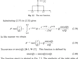
T R A N S F O R M O F R E C T( £ / 0 [B-3, W-27] The function r e c t ^ / g ) , shown in Fig.

2.2, is defined by

U l W1_*_{- « 2} _{< ' « 2 A}

( 2.3 7 )

(35)

2.5 S O M E F O U R I E R T R A N S F O R M S A N D T R A N S F O R M P A I R S 13

" 1 " ' _Q_

- Q/ 2 0 • Q/2 t

Fig. 2.2 The rect function.

Substituting (2.37) in (2.32) gives

Q/2

(t V

f .

w g-jnfQ _ eJ«fQ sin(nfQ)

J F r e c t — = e~j2_*ft_{dt =}_{= 6}

VG/ J •

-J2nf nfQ*

-Q/2

In like manner we obtain

9*

• w

^ V

fi-v e /

^ 0

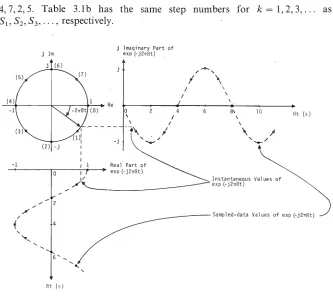
T R A N S F O R M O F s i N C ( r g ) [B-3, W-27] This function is defined by

(2.38)

(2.39)

(2.40)

The function sinc(f) is plotted in Fig. 2.3. The similarity of the right sides of (2.38) and (2.40) leads us to guess that

&[Q s i n c( r 0 ] = r e c t ( / / S ) (2.41)

' s i n e ( t ) T

[image:35.432.43.379.59.314.2]

\—*<-3 - 2 ~ \ . / - \ 'o / l 3 ^ - - " 4 t

Fig. 2.3 The sine function.

Taking the inverse transform of both sides of (2.41) gives (2.39), which verifies our guess. In like manner we obtain

2F~\Q s i n c ( / g ) ] = r e c t ( f/ 0 (2.42)

R E C T A N D S I N C F U N C T I O N P A I R S Combining the rect and sine function

trans-forms gives the following pairs:

r e c t( r / e ) ^ e s i n c ( / 0

g s i n c( / 0^ r e c t( / / 0

(2.43)

(36)

TRANSFORM OF ej2nfot_{Taking the Fourier transform of}_cxp(j2nf

0t) gives

(ej2nf0te-j2«ft) d t = H m

L s i n K

/ - /

Q

) P ] |

P-oo I <f~fo)P J P/2

# V2 7 r / o f_{= lim} P^oo

-P/2

The function in the braces in (2.45) is P s i n c [ ( / — f0)P], which is shown in Fig.

2.3. If the abscissa is changed to (f- f0)P in Fig. 2.3, the peak of the sine

function occurs at f0 and the first nulls occur at f0 ± l/P. As P oo the function

P s i n c [ ( / — /0) P } approaches infinite amplitude at the point f = f0- As P oo

the number of sidelobes of s i n c [ ( / — f0)P] becomes infinite for small but

nonzero distances \f — f0\ between / and f0. The amplitude of the sidelobes

approaches zero. These conditions correspond to the Dirac delta function, which has infinite height, infinitesimal width, and zero amplitude at all but one point. (For additional development of the delta function concepts, see distri-bution function discussions in [B-2, P-l].) We conclude that we can represent the Fourier transform of cxp(j2nf0t) by a delta function,

^eJ2nfot = d ( f_f o ) = h ' f=Jo (246)

10 otherwise

An equivalent definition of the Dirac delta function is that its width is zero, its height is infinite, and its area is unity. We can combine the concepts of infinitesimal width and unit area to show that the integral of the product of a delta function and another function yields the sampled value of the second function at the instant the delta function occurs. Applying this to the product of a frequency domain function X(f) and a delta function at f0 gives

X{f)d{f-f0)df=X{f0) (2.47)

Using (2.47) to find the inverse Fourier transform of S(f — f0) gives

^~1

S(f-fo) = S(f ~ fo)ej2nft

df = ej2nf0t

(2.48)

We can establish in like manner that 3Fb{t — t0) = exp( — j2nft0). The new pairs

are:

ej2nf0t_^d(f-f

0) (2.49)

5(t - t0) ^ e

-j 2 n f t o_(2.50)

TRANSFORM OF

cos(27i/

0

Since cos 9 = \{e

jd + e~jd

), the transform of ej9 , 9 = 2nf0t, determines the transform of cos 9. The transform of e

je_{is stated in}

(2.46); it yields

^ C O S( 2T C / OO = ^i(ej2_«f0t₊_{e ' ^ ) = \8{f + f}

(37)

2.5 SOME FOURIER TRANSFORMS AND TRANSFORM PAIRS 15

The inverse transform also follows from (2.49), leading to the Fourier transform pair

c o s ( 2 7 c/ o 0 « i 5 ( / + /0) + i 3 ( / - / o ) (2.52) TRANSFORM OF SIN(27E/00 Since sin 6 = (e

jd — e~je

)/2j, the transform of sin 6, 0 = 2nf0t, follows in the same manner as cos 6:

^ s i n ( 2 7 c/ o 0 = n ej 2 K f o t_{- e~^)/2j}_{= ( l / 2 / ) 5 ( / - / o ) -}_{O A / W + Zo)}

(2.53)

which leads to the Fourier transform pair

s i n ( 2 7 i/ o 0 ^ i / 5 ' ( / + / o ) - i / 5 ( / - / o ) (2-54) TRANSFORM OF A PERIODIC FUNCTION A periodic function with known period

P is represented by a Fourier series. Equation (2.1) is the Fourier series with real coefficients. Transforming the right side of (2.1) gives

z

fc=l

0 0

2nkt 2nkt akcos (- bk sin

CO •

Using the unit area of a delta function gives

(k/P) + e

fa* + A ) <s ( / - - ) # = fl

k

+ A

(2.55)

(2.56)

(Jc/i>)-£

where e is an arbitrarily small interval. The Fourier transform ofthe periodic function is thus an infinite series of delta functions spaced 1 /P Hz apart whose strengths are the Fourier series coefficients.

Transforming (2.14) yields

£ X(k)ei2nk,lf

= X X(k)d(f-k/P) (2.57)

Since X(k) = ak — jsign(k)bk, we again see that the Fourier transform of the

Fourier series gives spectral lines at / = 0, + l/P, ± 2/P,..± k/P,....

Figure 2.1 represents the Fourier transform coefficients if the vectors represent-ing X(k) are considered to be delta functions whose strengths are ak/2 and bk/2. TRANSFORM OF A SINGLE SIDEBAND MODULATED FUNCTION Single sideband

(38)

spectrum without duplicating the spectrum. This makes single sideband modulation more efficient than double sideband modulation which duplicates the spectrum.

Single sideband modulation is accomplished by multiplying a signal x(t) by the modulation factor exp( ±7*271/00- The Fourier transform of a modulated function is

^[x(t)e-j2nfot_{] =}x(t)e-j2nfot_e-j2n_^dt

x(t)exp[-j2n(f + f0)t] dt = X(f + f0) (2.58)

The inverse transform of X(f + f0) is found by a change of variables. Iff0 is fixed

and z =f + /0, then dz = df and

X(f + fo)ej2 *ft

df = X(z)ej2nzt_e-j2nfot_dz_(2.59)

The factor exp(— j2nf0t) does not vary with z and may be factored out of the

integral, giving the Fourier transform pair

x(t)e- J 2 n f o t ^X(f + fo) ( 2 6 Q) Equation (2.60) specifies a frequency shifted spectrum and the single sideband

modulation property is frequently called the frequency shift property. The shift for positive f0 is to the left. F o r example, consider the spectral value X(f0)

occurring at f0 in the original spectrum. The value X(f0) is found at / = 0 in the

shifted function X(f + /0).

TRANSFORM OF A TIME SHIFTED FUNCTION Suppose we have the Fourier

transform pair x(t) X(f) and want the Fourier transform of the time shifted function x(t — T). We find this transform by the change of variables z = t — T, which gives

# x ( £ - T ) = x(t - T)e~j27lft_{dt x(z)e-}j2nfx e~j2nfz

dz (2.61)

The factor e j 2 n f x_{does not vary with}_z_{and can be taken out of the integral,}

resulting in

&x{t - T ) = e-j2nfT_X(f)_(2.62)

The factor e~j2llfx

(39)

2.5 SOME FOURIER TRANSFORMS AND TRANSFORM PAIRS 17

imaginary parts of the Fourier transform spectrum. The result is the transform pair

x{t ± T) ++e±j2nfv_X(f)_(2.63)

TRANSFORM OF A CONVOLUTION Convolution is one of the most useful proper-ties of the Fourier transform in the analysis of systems incorporating an F F T . If

x(t) and y(t) are two time functions, their time domain convolution is represented symbolically as x{t) * y(t) and is defined as

x(t)*y(t) =

The Fourier transform of (2.64) gives

&[x(t)*y(t)] =

x(u)y(t — u) du (2.64)

J2nft _{x(u)y(t — u) du dt} _(2.65)

For most time functions the order of integration in (2.65) may be interchanged, giving

Letting z = t — u gives

#-[x(0*X01 =

x(u)

y{t - u)e-j2nft_dtdu

y(z)e-j2nf{z + u)_{dz du}

(2.66)

(2-67)

Note that u does not vary in the integration in brackets and may be factored out to give

&[x(t)*y(t)] = x(u) y{z)e-j2nfz

dz -j2nfu _(2.68)

The term in square brackets is the Fourier transform of y(t), which we denote

Y(f) = &Y(t). We now have

x(u)e-j2nfu_Y(f)du

(40)

The inverse transform also exists for most applications. Furthermore, we can interchange x(t) and y(t) in (2.69) and get the same answer. This establishes the Fourier transform time domain convolution pair

x(t)*y(t)~X(f)Y(f) (2.70)

If X(f) and Y(f) are two frequency domain functions, then frequency domain convolution is represented by X(f) * Y(f) and is defined as

X(f)*Y(f) = X(u)Y(f- u)du (2.71)

The inverse Fourier transform of X(f) * Y(f) is similar to the Fourier transform of x(t)*y(t) outlined in (2.64)-(2.70).

The transform pairs for time domain and frequency domain convolution are summarized as follows:

x(t)*y(t)~X(f)Y(f) (2.72)

x(t)y(t)^X(f)*Y(f) (2.73)

2.6 Applications of Convolution

The Fourier transform of a time domain convolution and the inverse transform of a frequency domain convolution are particularly useful for system analysis. The transfer function property illustrates the application of time domain convolution, and analysis of a function with unknown period illustrates the application of frequency domain convolution.

TRANSFER FUNCTIONS Determining transfer functions is an important appli-cation of the convolution property. Let a linear time invariant system have an input time function x(t) with transform X(f), as shown in Fig. 2.4. Let the system response to a delta function be the output y{t). Let the transform of y(t)

be Y(J).

I n p u t S y s t e m O u t p u t

X ( f ) Y ( f ) 0 ( f )

Fig. 2.4 Relationships between system transfer functions.

Y(f) is called a transfer function when used to describe a time invariant linear system. We shall demonstrate that the output time function o(t) has Fourier transform 0(f) given by

(41)

2.6 APPLICATIONS OF CONVOLUTION 19

as shown in Fig. 2 A Equation (2.74) gives the output time function o(t) as

o(t) = <F~i6{f) = ^-'XifiYif)

= x(t)*y(t) = x(u)y(t — u) du (2.75)

Most systems do not have an input until some specific time, which we can pick as zero so that

x(t) = 0, t<0 (2.76)

Furthermore, many systems do n o t have an output without an input (causal systems), so it is reasonable to set

y(t - u) = 0, t-u<0 (2.77)

Then

o(t) = x(u)y(t — u)du (2.78)

The integral in (2.78) may be approximated by a summation giving

K-l

o(K) « T £ x(n)y(K - 1 - n) (2.79)

n = 0

where o(n), x(n), andy(n) are the values of o(t), x(t), andy(t) at time t = n J7 a n d T

is an arbitrarily small time interval. Sampled functions x(n), y(ri), y{ — n), and

y(K— n) are shown in Fig. 2.5 for K= 12.

The function y(t) is called the impulse response of the system because an input

x(t) = S(t) produces the output y(t). We can approximate S(t) by a pulse Ts wide and 1 / T h i g h since both the delta function and pulse have unit area. A pulse with amplitude x(0)/T and duration T would give the output x(0)y(t — T) which, if sampled at times nT, would give the sampled sequence {x(0)y(n — 1)}. A pulse with amplitude x(0) and duration T will approximate the sequence

{Tx(0)y(n — 1)} if T is sufficiently small. Thus at sample K the output is

Tx(0)y(K — 1) due to an input x(0) at time 0. Likewise, at sample A" the output is

Tx(\)y(K - 2) due to an input x(l) at time T; it is Tx(2)y(K - 3) due to an input x(2) at time 2T; and in general, it is Tx(n)y(K — 1 — n) due to an input x(n) at time nT,n < K. A linear time invariant system has the property that the output at time KT is the sum of the outputs caused by all the inputs, so

K-l

o(K) = T £ x(n)y(K- 1 - n) (2.80)

(42)

. S a m p l e d I n p u t

A c t u a l I n p u t

12 16 n_{0 4}

y ( - n ) f y ( 1 2 - n )

A c t u a l I m p u l s e R e s p o n s e

M i l l

6( t )

- 4 0 - 4 0 4 8 1 2

' y ( t )

S y s t e m

Y ( f )

x ( t )

S y s t e m

Y ( f )

o(t)

Fig. 2.5 Sampled functions and system response.

invariant linear system with input x(t) and impulse response y(t) has output o(t).

The transform pair describing the transfer function property also holds under very general conditions. The transform pair follows:

o(t) = x(t) * y(t)

~

0(f) = X(f) Y(f) (2.81)

ANALYSIS OF A FUNCTION WITH UNKNOWN PERIOD The convolution property

is extremely useful for analyzing system outputs. W e shall illustrate this by analyzing the Fourier series of a function that actually has period P but for which a period Q was assumed because of lack of this knowledge. Knowledge of the periodicity of the input function is usually lacking when a system is mechanized, so the problem of transforming a function with period P under the assumption that the period is Q is a very real one.

Consider the system shown in Fig. 2.6 with the input cos(27i4f) + cos(27c5£). The Fourier transform of the input is delta functions with area \ a t / = — 5, — 4, 4, and 5 Hz. The 4 and 5 Hz terms together give a signal with the period P = 1 s, and using this to determine the complex Fourier series gives

X(k) = if k = + 4 or + 5

otherwise (2.82)

y (n₎_{S a m p l e d I m p u l s e}

Fast Transforms Algorithms, Analyses, Applications tqw darksiderg pdf

FAST TRANSFORMS

Algorithms, Analyses, Applications

Douglas F.

Elliott

K. Ramamohan Rao

CONTENTS

PREFACE

A C K N O W L E D G M E N T S

OF

A C R O N Y M S

N O T A T I O N

I N T R O D U C T I O N

x(n) =

^X{k)Un)

(1

-3)

<Mi)

FOURIER SERIES A M D THE FOURIER T R A N S F O R M

* 0

= ^ + I

40 =

f .

VG/ J •

-J2nf * nfQ

• w

^ V

L s i n K

/ - /

) P ] |

cos(27i/

0

fa* + A ) <s ( / - - ) # = fl

+ A

#-[x(0*X01 =

~

_^X{k)Un)

₍₁

_-3)

-J2nf nfQ*