UNIVERSITY OF LIVERPOOL Department of Mathematical Sciences
Ph. D. Thesis
Submitted in fulfillment of the requirements of the degree of
Doctor of Philosophy
Theoretical and Numerical Study on Optimal
Mortgage Refinancing Strategy
Author:
Jin Zheng
July 2015
This copy of the thesis has been supplied on condition that anyone who consults it is understood to
recognise that its copyright rests with its author and that no quotation from the thesis and no
Abstract
Contents
Abstract i
Contents iii
List of Figures iv
List of Tables v
Acknowledgement vi
1 Introduction 1
1.1 Research Objectives and Contributions . . . 1
1.2 Organization of this Thesis . . . 2
2 Preliminaries 4 2.1 General Introduction . . . 4
2.2 Basic Concept of Mortgage Contract . . . 6
2.2.1 The behaviour of the debtors . . . 6
2.2.2 Two basic types of mortgage contract . . . 7
2.3 Previous Work . . . 8
2.3.1 Structure-form . . . 8
2.3.2 Reduced-form . . . 11
2.4 Interest Rate Models . . . 12
2.4.1 Merton model . . . 12
2.4.2 Vacicek model . . . 12
2.4.3 CIR model . . . 15
2.5 Term Structure of Interest Rate . . . 16
2.5.1 Definitions . . . 16
2.5.2 The theories . . . 17
2.5.3 Interest rate derivative pricing: PDE approach . . . 18
3 Modelling of Refinancing 22
3.1 Business Economic Assumptions . . . 22
3.2 Model Setting for Mortgage Refinancing . . . 22
3.3 The Relationship Between Discrete Case and Continues Case . . . 39
4 Results for Various Models of Interest Rate 41 4.1 Merton Model . . . 41
4.1.1 T <∞. . . 41
4.1.2 T =∞. . . 47
4.2 Vasicek Model . . . 48
4.2.1 T <∞. . . 48
4.2.3 T =∞. . . 59
4.3 CIR Model . . . 60
4.3.1 Preliminary analysis . . . 61
4.3.2 T <∞. . . 61
4.3.3 T =∞. . . 67
5 Special Case: σ= 0 75 5.1 rt is a decreasing linear function . . . 75
5.1.1 T <∞. . . 75
5.1.2 T =∞. . . 76
5.2 rt is a piecewise function . . . 76
5.2.1 T <∞. . . 76
5.2.2 T =∞. . . 79
5.3 rt is a decreasing exponential function . . . 79
5.3.1 T <∞. . . 80
5.3.2 T =∞. . . 80
6 Remarks and Future Work 82
A Appendix of Tables 83
B Appendix: a new method to compute B(s, t) under Vasicek model 86
Bibliography 91
Index 91
List of Figures
4.1 The numerical value of E[Ms] under Merton model when T = 15 and
T = 30, where the value of the parameters are u=−0.001 and σ2 = 0.04. 67 4.2 The numerical value of E[Ms] with different parameters under Vasicek
model. . . 68 4.3 The numerical value of Var[Ms] with differentk under Vasicek model. . 68
4.4 The numerical value ofU
!
E[Ms],√ 1
Var[Ms]
"
under Vasicek model with
(a)ρ= 0.6, (b)ρ= 0.7, (c)ρ= 0.8, (d)ρ= 0.9. . . 69 4.5 Comparison Between c0 and Mortgage Rate Process for Small Volatility. 69 4.6 The numerical value of E[Ms] with different parameters under CIR model. 70
4.7 The numerical value of E[Ms] through different approximating methods
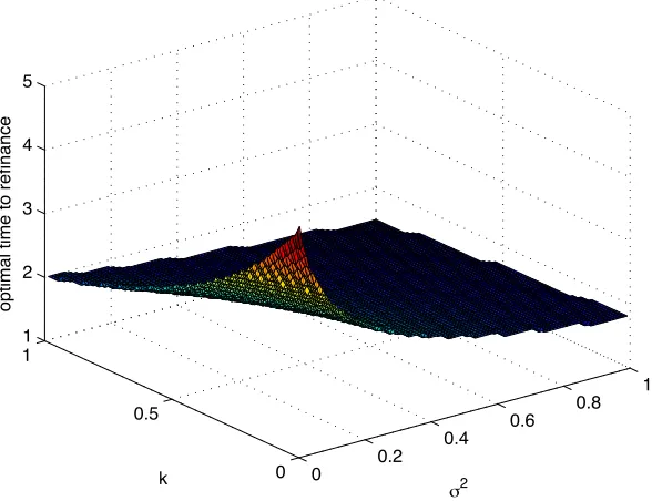
under CIR model. . . 70 4.8 The 3D Graph of Optimal Refinancing Time (ρ = 1) with the Change
of kand σ2 under CIR model. . . 71 4.9 The Optimal Refinancing Time (ρ = 1) with the Change ofkunder CIR
model. . . 71 4.10 The Optimal Refinancing Time (ρ = 1) with the Change of σ2 under
CIR model. . . 72 4.11 The numerical value of Var[Ms] with differentk under CIR model. . . . 72
4.12 The numerical value of Var[Ms] with differentσ2 under CIR model. . . 73
4.13 The numerical value of U
!
E[Ms],√ 1
Var[Ms]
"
under CIR model with
(a)ρ= 0.6, (b)ρ= 0.7, (c)ρ= 0.8, (d)ρ= 0.9 by the variation of k. . . . 73 4.14 The numerical value of U
!
E[Ms],√ 1
Var[Ms]
"
under CIR model with
(a)ρ= 0.6, (b)ρ= 0.7, (c)ρ= 0.8, (d)ρ= 0.9 by the variation of σ2. . . . 74 5.1 The numerical value ofMsunder Merton model withσ= 0 whenT = 15
and T = 30, with u1 = 0.001. . . 76
5.2 (a)The function of rt. (b)The value of Ms whenrtis a piecewise function. 77
List of Tables
A.1 The Relative Error of the approximation in Lemma 3.2.3, with y =
W(−ae−a)+a, whereW(z) is the product log function anda= x0
1−e−x0+
1−e−x0−x0
(1−e−x0)x0(x0−x) withx0 = 1.5. . . 83
A.2 The Optimal time to Refinance (with ρ= 1) under Vasicek model. The value of parameters are k= 1, θ= 0.03 and σ2 = 0.01. . . 84 A.3 The Optimal time to Refinance under Vasicek model based on the utility
function. The value of parameters are k = 1, θ = 0.03, σ2 = 0.01 and
T = 15. . . 84 A.4 The Optimal time to Refinance (with ρ = 1) under CIR model. The
value of parameters are k= 1, θ= 0.03 and σ2 = 0.01. . . 84 A.5 The Optimal time to Refinance under CIR model based on the utility
function. The value of parameters are k = 1, θ = 0.03, σ2 = 0.01 and
Acknowledgement
It would not be possible to finish this thesis without the guidance of my supervisors, the help from my friends, and the support from my family.
It is hard to express in words that how much I am indebted to my principle super-visor, Prof. Zhijian Wu, head of the Mathematical Sciences Department. I must offer my profoundest gratitude to Prof. Wu. It has been an honor to be his student. He offers his unreserved help and guides me to finish this thesis step by step. I appreciate all his contributions of time and ideas, the systematic guidance and great effort to make my Ph.D. experience productive. I admire his superb mathematical knowledge and rigorous attitude to the academic research. From him I have learnt a lot, not only about how to carry on a project, but also to view the academic and teaching work in a new perspective. For everything you have done for me, Prof. Wu, I can hardly convey my appreciation fully, but to say, thank you!
I would like to express my sincere gratitude to my second supervisors, Dr. Nan Zhang and Dr. Yiqing Chen. To Dr. Zhang, he has been invaluable on both an academic and a personal level. I especially want to thank him for sharing his thinking and experience. He has offered me tremendous expertise in scientific computing. To Dr. Chen, I am thankful to her for the help and support during my stay in Liverpool. I am indebted to her selfless support and love given to me during the Ph.D. study.
A very special thanks goes out to Dr. Dejun Xie, without his encouragement and support I could not have considered to chase for a Ph.D. career. It is Dr. Xie who introduced me into mathematical finance and provide me the idea for my project. He continuously contributed his thought into my study, for which I am extremely grateful. I would like to thank the Department of Mathematical Sciences at Xi’an Jiaotong-Liverpool University for financial, academic and technical support. The faculty of the department have provided me valuable experience in teaching and research. The library and computer facilities have been dispensable in Xi’an Jiaotong-Liverpool University.
I acknowledge my gratitude to the Department of Mathematical Sciences, University of Liverpool, who offers me the opportunity to start Ph.D research. They have offered me a three-month researching visiting to Liverpool. I have spent a wonderful time in UK and I will always miss the visiting.
during my graduate study. Special thanks to my very good friends Miss Yina Liu, Miss Lu Zong, and Mr. Yichen Liu. The meritorious suggestions and even challenges they provided benefit me a lot.
Chapter 1
Introduction
As one of the most frequently traded financial instruments, mortgage contract provides its debtors a way to manage their accounts. Valuation of mortgage security is of pivotal importance to investors, bankers and brokers in helping with their decision making from various perspectives. Knowledge of this kind is used as a key economic indicator not only in developed markets such as the US market, but also increasingly in emerging markets such as China and Brazil (see Lynn et. al [25]). The valuation of mortgage securities has to take into account the contracted choices to the debtors, among which refinancing is one of the most common choices. The main financial reason leading to refinancing, not taking into consideration the socioeconomic factors, is to take advantage of lower interest rate. There has been a great deal of research on the topic of modelling mortgage refinancing behaviours (see for example, Chen and Ling [9], Dunn and McConnell [13, 14], Lee and Rosenfield [21], Longstaff[23]).
1.1
Research Objectives and Contributions
This thesis presents a number of original contributions to the field of Mathematical Finance. These include:
1. An extension of the previous assumptions of constant discount factor (see Lee and Rosenfield [21], Dunn and McConnel[13], [14] et. al ) by suggesting that the discount factor is a stochastic process.
2. Presenting general models for the expected value and variance of the portfolio consisted of a loan and a refinancing agreement, which is applicable to all the affine interest rate models.
3. Redefining the optimal time to mortgage refinancing including risk.
4. A new asymptotic analysis for the expected value and variance of the portfolio.
5. Proposing a utility function approach describing the tradeoffbetween profit and risk, which makes the problem more realistic and applicable.
1.2
Organization of this Thesis
The contents of each chapter are outlined as follows.
Chapter 2: Preliminaries
We describe various views to capture the payment behavior of the debtors, and the methods that have been adopted to solve, either analytically or numerically, the value of the mortgage contract, or to make the refinancing decisions. First, we describe the approach named structure-form method, and then we represent the reduced-form approach. In addition, the term-structure of interest rates models are reviewed in this chapter.
Chapter 3: Modelling of Refinancing
We formulate some assumptions to support our methodology. To compromise the risk and the profit of refinancing, a utility function approach is proposed to describe the satisfaction of the debtors. In addition, we present general formulations to capture the expectation and the variance of the value of the contract.
Chapter 4: Results for Various Models
Chapter 5: Special case: σ= 0
We consider the special case that the volatility of the market interest rate is zero. We focus on the value of the contract and the optimal time the debtor may want to refinance. Variation analysis of the life of the contract is presented in this chapter.
Chapter 6: Remarks and Future Work
Chapter 2
Preliminaries
2.1
General Introduction
The pricing of mortgages in the context of stochastic interest rate plays an impor-tant role for financial management. The contributing factors impacting the value of mortgage contract have been explored by abundant literatures. As one of the most influential financial instruments in both the primary and secondary market, residential mortgage contract typically grants the debtor several options to facilitate his or he reaction to the market movement, among which the option of refinancing is of pivotal importance. In fact, a rather more common scenario in China’s market is that the ma-jority of mortgage debtors make periodical mortgage payment using their fixed income inflow from other sources, typically in the form of salary, for instance. This economy reality underscores the importance of the option of refinancing. (see Zheng et. al[48])
There has been a great deal of research on the topic of modelling mortgage refinance and prepayment behaviours. These works endeavoured to understand the conditions under which a debtor will pay back his or her outstanding debt before the end of the contracted period. Our motivation is different from most of the earlier work modelling the optimal mortgage prepayment problem. Their purpose was to determine the fair price of a mortgage contract under the condition that the loan may be prepaid or default. This mortgage contract pricing problem is closely related to the valuation of residential mortgage backed securities (MBSs) – an important problem as the MBS market has been one of the largest and fast-growing bond markets in the United States. One approach to the mortgage contract pricing is to view the prepayment or default opportunity as a built-in option in the mortgage contract that can be exercised by the debtor under favourable conditions. This approach inevitably borrows techniques from option pricing to calculate prices of mortgage contracts.
applied the binomial tree method to calculate the prices of the prepayment option and the mortgage contract. They considered the fixed-rate mortgage contract and assumed that a debtor would prepay the outstanding debt when the contract rate dropped deep enough. Their model incorporated the possibility of recursive refinancing. However, the optimal refinancing threshold rate (the rate under which refinancing, if takes place, will be optimal) cannot be obtained directly from the binomial tree. The optimal refinanc-ing threshold rates could only be approximated through multiple tests. The difference in basis point between this rate and the original contract rate was deemed as the value that the mortgage rate has to drop to make refinancing at present time optimal. The Longstaff-Schwartz ([24]) least-square Monte Carlo method is a well-known approach in option pricing to value the prices of multi-asset American options. In [23], Longstaff
used this method to compute the prices of the prepayment options and the mortgage contracts. More recently, Lee and Rosenfield ([21]) applied dynamic programming tech-nique to estimate the overall cost to the debtor refinancing the outstanding debt at a particular time with a new mortgage rate. The authors assumed that refinancing would happen if this cost was lower than the overall cost without refinancing.
2.2
Basic Concept of Mortgage Contract
2.2.1 The behaviour of the debtors
A mortgage is a type of legal agreement that conveys the conditional right of ownership on an asset or property by its owner (the debtor) to a lender (the mortgagee) as security for a loan. Virtually any legally owned property can be mortgaged, although real properties (land and buildings) are the most common (see [2]). Mortgage contracts typically carry a lower interest rate than other loans since the real property can act as a collateral. If the debtor suffers a worse financial condition and cannot afford to repay the loan, the lenders have the right to take over the assets, which is called default. The debtor also has the right to terminate the contact, the behavior of which is called prepayment or refinancing. This thesis will concentrate on the typical case of refinancing.
Prepayment refers to that behavior that the debtor chooses to settle all or part of the loan balances even though the lender’s preference may be to keep receiving the contracted continuous or periodical instalments, depending how the loan interest is collected (of course, real continuous collection of interest is not possible in banking practice)(see [43]). The main financial reason leading to prepayment, not taking into consideration socioeconomic factors, is typically the low investment return that the debtor may earn using the money at hand. That is, the available investment return for the debtor, on average, does not compensate his contracted continuous payment pledges to the lender. The studies on this aspect have seen important development recently, especially those contained in the paper of Xie et al ([46]), and Xie ([44], [45]), for instance, where the combination of advanced mathematical analysis with novelty numerical methods has made it possible to find very fast and cost effective solutions to the problem when the underlying interest rate is assumed as a specific but commonly adapted mean reverting model. (see Zheng et. al[48])
On the other hand, not all debtors have sufficient fund to make alternative invest-ment. The main reason for debtors to refinance is to improve the financial leverage efficiency by obtaining an alternative mortgage loan with a lower interest rate. Most of the previous literatures in this topic are empirical in nature from the perspective of optimal refinancing differentials, where the optimal differential is defined when the net present value of the interest payment saved reaches the sum of refinancing costs (see the paper of Agarwal et al ([3]) and relevant references contained therein). (see Zheng et. al[48])
day in the future. Relative to the case, it is more attractive to terminate the contract immediately than to wait for an optimal time. In our research, early termination is only considered for endogenous or financial reasons, based on the assumption that the value of the mortgage to the bank is equal to the total debt the debtor has to repay.
2.2.2 Two basic types of mortgage contract
Some of the following paragraphs are from ([1], [42]).
The two basic types of amortized loans are the fixed rate mortgage (FRM) and adjustable-rate mortgage (ARM). Fixed rate mortgages are prevalent because they allow the debtor to predict what the payments will be in the future over the duration of the loan. No matter what happens with interest rates, the payments won’t change if he or she has been involved in a fixed rate mortgage. This contrasts to the adjustable rate mortgages who do not have a fixed rate, leaving the debtor vulnerable and dependent upon the interest rate, which changes periodically. With a fixed rate mortgage, the debtor can calculate the amount of monthly payment, and the time he or she can pay off all the principal and interest. He or she will pay the same monthly payment during the life of the fixed rate mortgage contract. The monthly payment consists of three components, the fraction of principal balance, the interest rate payment and the transaction cost, or the service fee if the debtor wants to terminate the contract. The monthly payment in the fixed rate contract is higher than other mortgage choices, such as the fixed rate mortgage which offers the safety of knowing that the future payments will not increase.
The fixed rate mortgage is practical as it will not affect the debtor, if the rates increase. If the interest rates happen to decrease, it still will not affect the debtor as he or she can decide to refinance the loan to benefit from a better interest rate. An adjustable-rate mortgage differs from a fixed-rate mortgage in many ways. Most importantly, with a fixed-rate mortgage, the interest rate stays the same during the life of the loan. With an ARM, the interest rate changes periodically, usually in relation to an index, and payments may go up or down accordingly. The rate for an adjustable rate mortgage is determined by some market indices. Many adjustable rate mortgages are tied to the LIBOR, Prime rate, Cost of Funds Index, or other indices. A main reason to consider adjustable rate mortgages is that the debtor may end up with a lower monthly payment. The bank rewards him or her with a lower initial rate because the debtor is taking the risk that interest rates could rise in the future. However, the increase in mortgage payments can be significant if interest rates rise. Some debtors are unprepared for the increase in mortgage payments, and they may find themselves in dire financial straits when mortgage payments increase unexpectedly.
In financial terms, most literature considered the behaviour of the prepayment right which can be viewed as an American option. The debtor can prepay the loan at any time during the period of the contract. Compared to prepayment, refinancing is different since once the original is prepaid, the debtor may enter into another contract, and the payoffshould be minimized under this transaction (from one contract to another).
2.3
Previous Work
2.3.1 Structure-form
The measurement of prepayment incentive for option-based approach is endogenous. Many of the option-based approaches have been proposed, both in academic and prac-titioner sides. The termination behaviour is modelled as the optimal response of a rational debtor to the changes in some potential state variables, such as interest rate and house price. This type of model is closely related to value the early exercise fea-ture of American options. The previous literafea-ture assumes that the debtors will follow an optimal call strategy. A rational debtor will compare the liability and outstanding principal to make decisions of immediate refinancing or postponing for an additional period, where the liability to the debtor and asset to the lender are not differentiated. In these papers, (see Dunn and McConnell ([13], [14]), Bernnan and Schwarze ([8]), Kau et al ([19], [20]) and relevant references contained therein), the debtor followed the behaviour that he or she would exercise his or her call option whenever the value of mortgage exceeded the remaining balance plus transaction costs, while Stanton ([36]) argued that this approach was not suitable when we considered structural changes in the economic environment.
a positive effect.
Brennan and Schwartz have proposed a two-state variable model, including short rate and consol rate, to value the interest-dependent claims, i.e. default-free bonds and options, in the series of papers ([4], [5], [6], [7]). In [8], the authors priced GNMA securities through contrasting three different arbitrage-based models of the yield curve. The yield differentials were influenced by the interest-rate uncertainty and call policy. Transaction costs were introduced by Dunn and Spatt ([15]), Timmis ([38]) and Johnston and Drunen ([17]). As the debtors may refinance as many times as they can in the future, refinancing costs will reduce the incentive of refinancing. The model proposed by Dunn and Spatt ([15]), was developed to value the debt contract with refinancing. In their assumption, the immediate benefit from refinancing was equalled to the refinancing costs and call premium at the refinancing point. The bound on the pricing of debt contracts was obtained, and the method could be applied even if the debtor would like to refinance recursively with transaction costs. In addition, Dunn and Spatt ([15]) indicated a new method to handle transaction cost. The transaction cost could be regraded as a refinancing option, which will be included in the agreement or contract. The direction is of vital importance since it has significant influence on the subsequent research. However, the main shortcoming is that the model implies all of the bahaviours of refinancing occur simultaneously in the same pool.
Chen and Ling ([9]) followed the previous research and developed a dynamic model of mortgage refinancing in a contingent claim for fixed-rate mortgage. With a binomial interest rate process, they have solved (1) the optimal mortgage refinancing strategy, (2) the value of the refinancing option, (3) the value of the mortgage liability to the debtor, and (4) the value of the contract, simultaneously. They assumed that a debtor would prepay the outstanding debt when the present value of interest rate savings exceeded the refinancing costs. Their model incorporated the possibility of recursive refinancing. IDF (interest rate differentials between the current market rate and contract rate) was first demonstrated in this paper, and the results of which contained the required minimum IDF for refinancing. The result showed that the IDF would increase with transaction costs, interest rate volatility and debtor’s expected holding period.
Stanton ([36]) observed the drawbacks of reduced-form models, and the major one of which was that the prepayment model had low out-of-sample forecasting power. Stan-ton ([36]) incorporated both rational and exogenously determined prepayment strate-gies. He estimated heterogeneity in transaction cost faced by the debtors. Compared to Dunn and McConnell ([13], [14]), Dunn and Spatt ([15]), Timmis ([38]), Johnston and Drunen ([17]) et al, Stanton ([36]) assumed that the debtor would make decisions at discrete time. He acknowledged that some debtors would prepay even their coupon rate was below current rate, which meant these debtors failed to repay even at the optimal time. The model gave a simple model for rational prepayment, which was allowed to address the consequence of a structural shift in economic, such as seasonality.
Stanton and Wallace ([37]) developed the first contingent claims mortgage valuation algorithm of self-election, which allowed the debtors to choose the different fixed-rate loans with combinations of coupon rate and points, and an equilibrium model was proposed with transaction costs. Although some literature have investigated the sim-ilar problem before (see Yang ([47]), Leroy ([22])), they were unable to construct an equilibrium in multiple refinancing. The numerical solutions in the paper [37] demon-strated that, in determining the optimal menu of the mortgage contracts, the shape of yield curve, the transaction cost and the mobility of the debtors played an significant important role.
As the past option-based models focused on trying to predict future cash flows, Kalotay et al ([18]) concentrated on the market value of MBS. The reasons for the fail-ure of past option-based models were as followings. The previous models either used Treasury or swap curves to model the behaviour refinancing. However, these curves could not accurately reflect the actual cost of funds, which led to the fact that the past option-based models were not able to explain and match market MBS prices. Instead, Kalotay et al ([18]) used two different yield curves, one for discounting mortgage cash flows and the other for MBS cash flows. By assuming that the sole purpose of refi-nancing was to save interest expense, they modelled the full spectrum of refirefi-nancing behaviour by a notion refinancing efficiency. They demonstrated that a rigorously con-structed option-based model could accurately explain the market price and MBS were well priced when most debtors exercise their refinancing option near-optimally.
Longstaff([23]) studied the optimal recursive refinancing problem. They used the two-factor term structure model to describe interest rate fluctuation. The remarkable improvement was that the approach incorporated three factors on the optimal refinanc-ing strategy: transaction cost, the probability of prepayrefinanc-ing for exogenous reasons and the debtor’s financial situation. Longstaffborrowed method in Longstaffand Schwartz ([24]) to compute the prices of the prepayment options and the mortgage contracts. The results illustrated that it was optimal to delay prepayment for the debtor beyond the point when compared to the conventional models.
2.3.2 Reduced-form
Considering the fact that the debtors prepay their loans even the prevailing refinanc-ing rate exceeds their initial contract rate, and other debtors do not prepay when the initial contract rate exceeds the prevailing rate, Schwartz and Torous ([31]) have mod-elled the factors such as economic, demographic and geographic elements, which would influence the debtor’s decision by statistical estimation. Schwartz and Torous ([31]) incorporated an empirical prepayment function into a two-factor default-free interest-dependent claim and led to a partial differential equation for the value of mortgage contract. One significance is that in this research, it is recognized that at each time, there exists a probability of prepaying, that the random time when a debtors prepays could be described as a hazard rate model. They provided a complete model to value the MBS. The later work of Schwartz and Torous ([32]) was the first to introduce the possibility of default and investigate the interaction of prepayment and default decisions for valuing MBS. With transaction costs, the conditional probability of prepayment or default was given by the function of prepayment or default, separately. In an arbi-trage free market, the value of the mortgage or mortgage pass-through satisfied the second-order partial differential equation. Although some of the reduced-form models can be quite complicated, it is straightforward to use the Monte Carlo simulation. In 1993, Schwartz and Torous ([33]) took advantage of Poisson regression to estimate the parameters of a proportional hazards model instead of likelihood method, which was more efficient to obtain the result.
extended the unified economic model to analyze the heterogeneity among debtors, which was quite important in accounting for their prepayment and default behaviour.
2.4
Interest Rate Models
2.4.1 Merton model
Merton ([27]) proposed the following simplest stochastic process for the dynamic of interest rate
rt=r0+ut+σWt,
where theuandσare constants, andWtis the standard Brownian process. Asrtfollows
the normal distribution with mean r0+ut and variance σ2t, the moment generation
function of rt is
Mrt(z) =e
(r0+ut)z+12σ2z2t.
The first and second moments of rt are unbounded, which allow the interest rate rt to
be infinity. In a sense, the model lacks stability and cannot be applicable to all the conditions.
2.4.2 Vacicek model
The Vasicek model was introduced by Vasicek in 1977 ([39]). This model can be used to interest rate derivative valuation and also adapted to credit market. Vasicek Model is an Ornstein-Uhlenbeck stochastic process given by
drt=k(θ−rt)dt+σdWt,
where reversion ratek, long-term mean level θ, volatilityσ are positive constants, and
Wtis the standard Brownian process. Vasicek model was the first one to capture mean
reversion, which defined an elastic random walk around the trend.
• θ: ’long term mean level’. The long run equilibrium value towards which the interest rate goes back, which means all future trajectories ofrtwill evolve around
a mean levelθ in the long run.
• k: ’speed of reversion’. It gives the adjustment of speed and has to be positive in order to maintain stability around for the long-term value.
• σ: ’instantaneous volatility’. It determines the volatility of the interest rate, and higherσ implies more randomness.
• k(θ−rt)dt: ’drift term’. The drift factor that describes the expected change in
• σ2
2k: ’long term variance’. All future trajectories of rt will revert around the long
term mean with such variance after a long time.
When rt goes under θ, the drift term k(θ −rt) becomes positive, generating a
tendency for the interest rate to move upwards, and vice versa.
Vasicek model was the first one to capture mean reversion property of the interest rate. Unlike stock price, the model assumes interest rate moves within a limited range, which shows tendency of the interest movement will finally revert to a long run value. However, the main drawback of Vasicek model is that the short term interest rate can become negative, which is not acceptable at the economic point-of-view.
Vasicek model yields an explicit formula
rt=θ+ (r0−θ)e−kt+σe−kt # t
0
ekudWu,
with
E[rt] =θ+ (rs−θ)e−kt
Var[rt] =σ2e−2ktE
$ !# t
0
ekudWu
"2%
=σ2e−2ktE
&# t
0
e2kudu
'
= σ
2
2k
(
1−e−2kt).
One can see thatrtis a Gaussian random variable. This follows from the definition of
the stochastic integral termσe−kt*t
0ekudWu, which is lim||Π||→0+in=0−1σe−k(t−ui) ,
Wui+1 −Wui
-. As the increment is Wui+1−Wui∼N(0, ui+1−ui),
*t 0e2
kudW
u is Gaussian.
As rt follows normal distribution with mean of θ+ (r0 −θ)e−kt and variance of
σ2
2k
,
1−e−2kt
-, the moment generating function ofrt is
Mrt(z) =e(
θ+(r0−θ)e−kt)z+σ2
4k(1−e−
2kt)z2
.
Compare to Merton Model, Vasicek Model avoids the infinite interest rate. However, the main disadvantage of Vasicek Model is that interest can be negative. Whent→ ∞, we have
⎧ ⎪ ⎨
⎪ ⎩
lim
t→∞E[rt] =θ
lim
t→∞Var[rt] =
σ2
2k.
As the explicit formula is given, one can obtain the zero-coupon bond price in the following way in the paper of Mamon ([26]). Using the risk-neutral valuation framework, the price of a zero-coupon bond with maturityT at timet is
B(t, T) = E2e−!tTrudu|Ft
3
.
We let Xt=rt−θ, as Xt is the solution of the Ornstein-Uhlenbeck equation, we have
with the initial value
X0=r0−θ.
Applying Ito’s lemma formula,Xt is given by
Xt=e−ktX0+σe−kt # t
0
eksdWs,
with
E[Xt] =e−ktX0
Cov[Xt, Xu] =σ2e−k(u+t)E
&# t
0
eavdWv
# u
0
eavdWv
'
.
=σ
2
2ke
−k(u+t)(e2k(u"
t)−1)
As Xu is a Gaussian process with continuous sample paths, then
*t
0X(u)du is also
Gaussian, with
E
&# t
0
Xudu
'
=
# t
0
E[Xu]du=
X0
k
(
1−e−kt)
Var
&# t
0
Xudu
'
=Cov
&# t
0
Xudu,
# t
0
Xvdv
'
=
# t
0 # t
0
Cov[Xu, Xv]dudv
=σ
2
2k3 2
−e−2kt+ 4e−kt+ 2kt−33.
Since ru =Xu+θ, we have
E
&# T
t
rudu
'
=E
&# T
t
(Xu+θ)du
'
=−rt−θ
k
(
1−e−k(T−t))+θ(T −t)
Var
&# T
t
rudu
'
=Var
&# T
t
Xudu
'
=σ
2
2k3 2
−e−2k(T−t)+ 4e−k(T−t)+ 2k(T −t)−33.
Thus, the value of the zero-coupon bond price can be described as
B(t, T) = E2e−
!T
t rudu|Ft
3
=E2e−
!T t rudu|rt
3
=e[−!tTrudu]+
1 2Var[−
!T t rudu] =A1(t, T)e−A2(t,T)rt,
where
A1(t, T) = exp !!
θ−σ
2
2k
"
[A2(t, T)−(T −t)]−
σ2A22(t, T) 4k
"
A2(t, T) =
1−e−(T−t)k
2.4.3 CIR model
The CIR short term interest rate process, first proposed by Cox et al ([10]), is a mathe-matical model describing the evolution of interest rate. The model specifies that under the risk-neutral measure Q, the instantaneous interest rate follows the stochastic dif-ferential equation:
drt=k(θ−rt)dt+σ√rtdWt. (2.1)
CIR model is one of the most well-known and widely used models for interest rate and the pricing of interest rate derivatives, by which many books and books have adopted to capture the term structure of interest rate (see Shreve ([35]), Dunn and McConnell ([13], [14]), Sharp ([34]), Miranda-Mendoza ([28]) et al). It is composed of one deterministic term and one random term. The deterministic term (also ’the drift term’) is chosen to produce the so called ’mean-reverting’ property, which means that if the interest rate is larger than the long-term mean, the drift term will be negative so that the interest rate will be pulled down in the direction of the long-term mean. However, if the interest rate is smaller than the long-term mean, the drift term will be positive so that the interest rate will be pulled up in the direction of the long-term mean. And the random term is to model the volatility caused by unpredictable factors. In (2.1), k is the reversion rate, which refers to the speed measuring how fast the process will be reverted back to the mean once it evolves away from the mean, while
θ is long−term mean interest rate and σ is the standard deviation, all of which are
positive constants. When we add one condition 2kθ >σ2, the interest rate is always positive, otherwise the interest rate can reach zero. The volatility termσ is multiplied with the term√rt, which eliminates the probability of negative interest rates compared
to the Vasicek model. The main reason to adopt CIR model to generate the mortgage rate is that it avoids the negative rates, and corresponds to empirical observations that higher interest rates are associated with higher volatility, which guarantee that our simulated mortgage rate is more realistic. The probability density function of rs,
conditional onrv, wheres > v, is given by Cox et al ([10])
frs|rv(x) =ae
−brv−ax
!
ax brv
"c2
Ic
(
24abrvx
)
, x >0 (2.2)
where
a= 2k
σ2,
1−e−k(s−v)-, b=ae
−k(s−v), c= 2kθ
σ2 −1,
and Ic(y) is the Modified Bessel’s function of the first kind of orderc, which is
Ic(y) =
∞ 5
m=0 ,y
2 -2m+c
Based on (2.2), we can calculate the moment generating function as
Mrs|rv(t) = E6
etrs
|rv
7
=
# ∞
0
etxae−brv−ax
!
ax brv
"c2
Ic
(
24abrvx
)
=
# ∞
0
ae−brv
!
a brv
"2c ∞ 5
m=0 ,√
abrv-2 m+c
m!Γ(m+c+ 1)e
−axxc
2x 2m+c
2 etxdx
=
# ∞
0
ae−brv
!
a brv
"2c ∞ 5
m=0 ,√
abrv
-2m+c
m!Γ(m+c+ 1)e
−(a−t)xxm+cdx
=ae−brv
!
a brv
"c2 ∞ 5
m=0 ,√
abrv
-2m+c
m!Γ(m+c+ 1)Γ(m+c+ 1)
!
1
a−t
"m+c+1
=
∞ 5
m=0
e−brvbrm
v am+c+1
1
m!
!
1
a−t
"m+c+1
=
!
a a−t
"c+1 ∞ 5
m=0
e−brv
(
abrv
a−t
)m
m! =
!
a a−t
"c+1
ebrv ta−t,
and specifically, the moment generating function ofrs, conditional onr0 (ie, v= 0), is
Mrs(t) =
!
a a−t
"c+1
e
br0t a−t, where
a= 2k
σ2(1−e−ks), b=ae
−ks, c= 2kθ
σ2 −1.
In addition, the zero-coupon bond price based on CIR model is given in the following section.
2.5
Term Structure of Interest Rate
For more details, the reader may refer to Gibson et al [16]).
2.5.1 Definitions
In the rational financial market, a lender will never lend money for free. As the value of money is always higher today than future, the lender will charge for borrowed money as the compensation for the loss of the future opportunities one could miss out for the borrowed money.
discount bond price of zero-coupon bond from current timet to the maturity time T. At timet, the yield to maturity R(t, T) of the discount bondB(t, T) follows
B(t, T)e(T−t)R(t,T) = 1,
and thus,R(t, T) is represented as,
R(t, T) =−ln [B(t, T)]
T −t , (2.3)
where R(t, T) is the continuously compounded interest rate. When we fix t, one can see that the yield curve is determined by T.
We define r(t) as the spot rate at time t, then
r(t) = lim
T→tR(t, T) =−∆limt→0R(t, t+∆t)
=− ln [B(t, t+∆t)]
∆t .
AsB(t, t) = 1, we have
r(t) =−dln [B(t, T)]
dT |T=t.
We denote f(t, T1, T2) as forward rate, which can be agreed on the current time t
for a risk-free loan from T1 to T2. Similarly, the instantaneous forward rate is
f(t, T) =−dln [B(t, T)]
dT , (2.4)
which gives
B(t, T) =e−!tTf(t,u)du.
Note that in our thesis, we only focus on the short rate model, which is given by the following stochastic differential equation
drt=u(t, rt)drt+σ(t, rt)dWt,
which impliesrtis a Markov process, and the zero-coupon bond price given by
B(t, T) = E2e−!tTrsds|Ft
3
.
2.5.2 The theories
bond maturating at timeT should be equal to the geometric average of the short-term rate fromtto T.
The Market Segmentation Theory: The key assumption of this theory is that bonds of different maturities are not substitutes at all. It implies markets are completely segmented, and interest rate at each maturity are determined separately. As bonds of shorter holding periods have lower inflation and interest rate risks, segmented market theory predicts that yield on longer bonds will generally be higher, which explains why the yield curve is usually upward sloping.
The Liquidity-Preference Theory: The liquidity premium theory views bonds of different maturities as substitutes, but not perfect substitutes. Investors prefer short rather than long bonds because they are free of inflation and interest rate risks. This implies that the prices of longer-term bonds tend to be more volatile than the prices of short-term bonds, resulting in a higher expected return, or risk premium, to offset the higher risk.
2.5.3 Interest rate derivative pricing: PDE approach
Recall that we denoteB(t, T) as the discount bond price of zero-coupon bond. In the risk-neutral world, one can defineB(t, T) as (see Shreve ([35]))
B(t, T) = E2e−!tTrsds|Ft
3
.
We assume in the general case, the interest rate follows
drt=u(t, rt)drt+σ(t, rt)dWt,
whereu(t, rt) andσ(t, rt) are functions related totand rt.
We consider the short term rate is the single factor deriving the term structure (see Gibson et al [16]). Thus, we can derive a PDE for valuation B(t, T), whose value is a function of interest ratert, time tand maturity date T. Applying Ito lemma ([35]) to
the functionB(t, T), we obtain that
dB=∂B
∂tdt+ ∂B ∂rt
drt+
∂2B ∂rt2 (drt)
2
=a(t, rt)dt+b(t, rt)dWt,
with
a(t, rt) =a=
∂B
∂t +u(t, rt) ∂B ∂rt
+1 2σ
2(t, r
t)
∂2B
∂rt2 (2.5)
b(t, rt) =b=σ(t, rt)
∂B ∂rt
.
Now construct a portfolio Π, which consists of long one asset B1 and short ∆ of B2.
Thus
The change in the portfolio overdt is
dΠ=dB1−∆dB2
=(a1−∆a2)dt+ (b1−∆b2)dWt.
To eliminate the risk of the portfolio, we choose
∆= b1
b2.
As the return on an amount Π invested in riskless assets would see a growth of rΠdt
in a timedt.
rΠdt= (a1−
b1
b2a2)dt,
which gives
a1−rB1
b1
= a2−rB2
b2
. (2.6)
As the (2.6) holds for any pair of B1 and B2, the ratio of a−brB needs to be only concerned withrand t. We denote the market premiumλ(r, t) = a−rB
b . In compatible
with the no-arbitrage requirement, we can assume that λ(r, t) = 0, which gives
a=rB, (2.7)
whereais defined in equation (2.5). Substituting equation (2.5) into (2.7), we have
∂B
∂t +u(t, rt) ∂B ∂rt
+ 1 2σ
2(t, r
t)
∂2B
∂rt2 −rtB = 0, (2.8)
We can guess the solution with the form of
B(t, T) =A1(t, T)e−A2(t,T)rt.
Thus
∂B ∂t =A
′
1(t, T)e−A2(t,T)rt−A1(t, T)A′2(t, T)rte−A2(t,T)rt
∂B ∂rt
=−A1(t, T)A2(t, T)e−A2(t,T)rt
∂2B
∂rt2 =A1(t, T)A
2
2(t, T)e−A2(t,T)rt,
where
A′1(s, t) = dA1(t, T)
dt , A
′
2(s, t) =
dA2(t, T)
We adopt Merton’s Model as an example, where u(t, rt) =u and σ(t, rt) = σ, and
plug ∂∂Bt, ∂∂rB t,
∂2B
∂r2
t in (2.8) gives
A′1(s, t)−uA1(s, t)A2(s, t) +
1 2σ
2A
1(s, t)A22(s, t)− 6
A1(s, t)A′2(s, t) +A1(s, t) 7
rt= 0.
(2.9)
As the (2.9) holds for all rt, we can figure out that
⎧
⎪ ⎪ ⎨
⎪ ⎪ ⎩
A′1(s, t)−uA1(s, t)A2(s, t) +1 2σ
2A
1(s, t)A22(s, t) = 0
A1(s, t)A′2(s, t) +A1(s, t) = 0.
(2.10)
With the boundary conditionsA1(T, T) = 1 and A2(T, T) = 0, we can obtain
A1(t, T) = exp
!
−u(T−t)
2
2 +
σ2(T −t)3 6
"
A2(t, T) =T −t.
Similar calculation can be worked out with Vasicek Model and CIR Model, and the results are as followings: For Vasicek Model, we have
A1(t, T) = exp !!
θ− σ
2
2k2 "
[A2(t, T)−(T−t)]−
σ2A22(t, T) 4k
"
A2(t, T) =
1−e−(T−t)k
k .
For CIR Model, we have
A1(t, T) = 8
2ωe(k+ω)(2T−t)
2ω+ (k+ω)6
e(T−t)ω−17 92σkθ2
A2(t, T) = 2
6
e(T−t)ω−17
2ω+ (k+ω)6
e(T−t)ω−17
ω=4k2+ 2σ2.
2.5.4 Feynman-Kac formula
The Feynman-Kac formula (see [41]) establishes a link between parabolic partial dif-ferential equations (PDEs) and stochastic processes.
Theorem 2.5.1. Let Xt be a stochastic process satisfying
dXt=u(Xt, t)dt+σ(Xt, t)dWt.
Let F(Xt, t) be the price at time of t of any derived security in the economy maturing
at T , with the maturity price
and one can derive a PDE ∂F
∂t +u(t, x) ∂F
∂x +
1 2σ
2(t, x)∂2F
∂x2 −V(t, x)F = 0,
with the boundary condition
F(T, x) =g(x) for all x.
Then the Feynman − Kac formula tells us that the solution can be written as a
condi-tional expectation
F(t, x) = E2g(xT)e−
!T
t V(u,Xu)du|Xt=x
3
.
Proof. We assume F(t, x) is the solution of the PDE, and we construct
Y(s) =e−
!s
t V(u,Xu)duF(s, Xs). Apply Ito’s Lemma, we have
dY(s) =F(s, Xs)de−
!s
t V(u,Xu)du+e− !s
t V(u,Xu)dudF(s, Xs) +de− !s
t V(u,Xu)dudF(s, Xs) =F(s, Xs)de−
!s
t V(u,Xu)du+e− !s
t V(u,Xu)dudF(s, Xs) =e−!tsV(u,Xu)du[−V(s, Xs)F(s, Xs) +dF(s, Xs)]. As
dF(s, Xs) =
∂F ∂sds+
∂F ∂xdx+
∂2F ∂x2(dx)
2
=∂F
∂t +u(s, Xs) ∂F
∂x +
1 2σ
2(s, X
s)
∂2F
∂x2 +σ(s, Xs)
∂F ∂xdW,
dY(s) can be continued as =e−
!s
t V(u,Xu)du
&
−V(s, Xs)F(s, Xs) +
∂F
∂s +u(s, Xs) ∂F
∂x +
1 2σ
2(s, X
s)
∂2F
∂x2 +σ(s, Xs)
∂F ∂xdW
'
=e−
!s
t V(u,Xu)duσ(s, Xs)∂F
∂xdW.
Integrating this equation fromtto T, we can obtain that
Y(T)−Y(t) =
# T
t
e−!tsV(u,Xu)duσ(s, Xs)∂F
∂xdW.
Taking the expectation, conditioned onXt=x of both sides implies
E[Y(T)|Xt=x] = E[Y(t)|Xt=x] =F(t, x).
Thus
F(t, x) =E2F(T, XT)e−
!T
t V(u,Xu)du
3
=E2g(xT)e−
!T
t V(u,Xu)du|Xt=x
3
.
One can see that when the payoff g(xT) = 1, the formula can be adopted to the
Chapter 3
Modelling of Refinancing
3.1
Business Economic Assumptions
As market increasingly diversifies, the mortgage contract itself becomes rather com-plicated in real industry, the documentation of which concerns not only financial and business consultants, but also commercial lawyers and regulatory compliance, etc. This said, it is reasonable for us to summarise common contract specifics and economic en-vironment in which the mortgage deals are cultivated.
1. With the continuous payment, one refinancing is granted throughout the whole during of the original contract. The transaction fee is charged as the percentage of the profit gained by refinancing. If the profit isMs, the lender may charge the
transaction fee asβMs, with β ∈(0,1). In addition, the life of the contract will
not be affected by refinancing.
2. No prepayment or default will be considered in this thesis.
3. The market is complete, and both the lender and the debtor have equal access to the market information.
4. The debtor does not have a sizable enough amount of fund to make early payment.
Among these assumptions, 1-2 are contract clauses or interpretations of these clauses; and 3-4 are market and economic environment assumptions. In particular, the as-sumption 3 guarantees the method and solutions contained in this thesis are arbitrage free.
3.2
Model Setting for Mortgage Refinancing
1. rt: market interest rate at time t, we define e−
!s
0rtdt as the discount process to times.
3. c(t) = ct: mortgage rate contracted at t, for the time interval [t, T]. ct is a
deterministic function of rt.
4. P(t): Consider a bank loan of amount P(0) at t = 0 for the duration of T.
P(t) is the principal balance at time t, which implies if the debtor wants to pay off the debt at time t, he or she needs to repay P(t). Therefore, P(t) equals
P(0) 1−e−c0T
,
1−e−c0(T−t)- and at maturity datet=T,P(T) = 0.
5. mt: rate of payment per unit amount of loan determined at tfor the duration of
[t, T]. The payment rate per unit amount and the mortgage rate satisfy
# T
t
e−ct(s−t)m
tds= 1,
which gives
−mt
1
ct
e−ct(s−t)
: : : :
T
t
= mt
ct
(
1−e−ct(T−t)
)
= 1,
or equivalently
mt=
ct
1−e−ct(T−t). (3.1)
6. We consider a portfolio V consisting of a loan of P(0) at time t = 0 for the duration ofT years with the mortgage rate c0 and a refinancing agreement to be
exercised at time s ∈ (0, T), if the mortgage rate cs at time s satisfies cs < c0.
Initially, the debtor would undertake the continuous payment rate of m0P(0)
with the mortgage rate c0. At time t = s, if refinancing is exercised leads to a
new payment rate ofmsP(s) with the mortgage ratecs. IfMs is the value of this
portfolio at timet= 0, with the market interest rate rs at times, we have
Ms=
⎧
⎪ ⎪ ⎨
⎪ ⎪ ⎩
# T
s
[m0P(0)−msP(s)]e−
!t
0rvdvdt c
s< c0
0, cs≥c0,
(3.2)
where
m0P(0)−msP(s) =P(0)
$
c0
1−e−c0T −
cs
6
1−e−c0(T−s)7
[1−e−c0T]61−e−cs(T−s)7
%
.
Ms can be also viewed as the total discounted profit of refinancing at time s. As
described, the lender may chargeβMsas the transaction fee. Thus, the profit gained by
the debtor is (1−β)Ms. A natural question is to find the optimal time which maximizes
its expectation E[Ms] and its variance Var[Ms] as key factors. If U: R2 →Ris such a
utility function, our problem is equivalent to
U
8
E[Ms],
1
4
Var[Ms]
9
, (3.3)
where
E[Ms] =
# T
s
E2[m0P(0)−msP(s)]e−
!t
0rvdv
3
dt, (3.4)
and
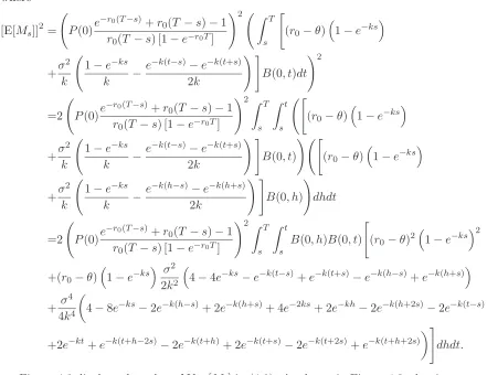
Var[Ms] = E
$
[m0P(0)−msP(s)]2
!# T
s
e−!0trvdvdt
"2%
−(E[Ms])2. (3.5)
In general, the unconstrained maximization problem U(x, y) will be obtained by setting Ux = 0 and Uy = 0, with the second-order conditions Uxx < 0, Uyy < 0 and
: : : :
Uxx Uxy
Uxy Uyy
: : : :
< 0. Thus, for a utility function U(x, y), we can see that
: : : :
Uxx Uxy
Uxy Uyy
: : : :
is a
negative-definite matrix.
We let x(s) = E[Ms] andy(s) = √ 1
Var[Ms]
in (3.3), thus, the optimal point will be obtained by
d
dsU(x(s), y(s)) =Uxx
′(s) +U
yy′(s) = 0, (3.6)
because
d2
ds2U(x(s), y(s))
=Uxx
6
x′(s)72+ 2Uxyx′(s)y′(s) +Uxx′′(s) +Uyy
6
y′(s)72+Uyy′′(s)
=,
x′(s), y′(s) -!
Uxx Uxy
Uxy Uyy
" !
x′(s)
y′(s)
"
+,
Ux, Uy
-!
x′′(s)
y′′(s)
"
<0,
thus, the maximum value of U(x(s), y(s)) will occur at ssatisfying (3.6).
In particular, The utility function can be described by the Cobb-Douglas model (see [40]), where
U
8
E[Ms],
1
4
Var[Ms]
9
= (E[Ms])ρ
1
( 4
Var[Ms]
)1−ρ, (3.7)
whereρ∈(0,1).
Without loss of generality, we assume E[Ms] and Var[Ms] are continuous,
posi-tive and differentiable. The maximum value of U
!
E[Ms],√ 1
Var[Ms]
"
will occur at s
satisfying dU
ds = 0, implying
ρ d
dsln (E[Ms]) = (1−ρ) d dsln
(4
Var[Ms]
)
Withρ= 1, the maximum value of U
!
E[Ms],√ 1
Var[Ms]
"
will occur at ssatisfying
dE[Ms]
ds = 0.
We assume the mortgage rate ct is a function of rt with ct ≥ rt, and the market
interest ratertsatisfies the following SDE of
drt=u(t, rt)dt+σ(t, rt)dWt,
where u(t, rt) is the drift coefficient, σ(t, rt) is the diffusion coefficient, and Wt is the
standard Brownian motion.
The expectation of Ms can be represented as
E[Ms] =
# T
s
E2[m0P(0)−msP(s)]e−
!t
0rvdv
3
dt
=
# T
s
E2E2[m0P(0)−msP(s)]e−
!t
0rvdv|r
s
33
dt
=
# T
s
E2[m0P(0)−msP(s)]e−
!s
0rvdvE
2
e−!strvdv|rs
33
dt
=
# T
s
E2[m0P(0)−msP(s)]e−
!s
0rvdvB(s, t)3dt, (3.9)
where B(s, t) = E2e−!strvdv|rs
3
is zero-coupon discounted bond price with maturityt
with explicit formula
B(s, t) =A1(s, t)e−A2(s,t)rs.
And the formulae of A1(s, t) and A2(s, t) will depend on the stochastic interest rate process we adopted.
We can rewrite (3.9) as
E[Ms] =E
&
[m0P(0)−msP(s)]e−
!s
0 rvdv
# T
s
B(s, t)dt
'
=E
$
[m0P(0)−msP(s)]e−
!s
0 rudu lim
||Π||−→0
n
5
i=0
B
!
s, i
n(T −s)
"
T−s n
%
.
We construct a portfolio Bs = lim||Π||−→0 +n
i=0B ,
s,ni(T−s)-T−s
n , and the
pay-ment rate of the portfolio after refinance at timesdenotes asRs=
cs[1−e−c0(T−s)] [1−e−c0T][1−e−cs(T−s)]. Thus, we have
E[Ms] =E
2
P(0) (R0−Rs)Bse−
!s
0 rvdv
3
.
We may think the debtor holds a payment option. If the mortgage rate at time s,
cs, is lower than the contractual rate, c0, which implies Rs < R0, the debtor would
like to exercise the option and new payment becomes P(0)RsBs, making a profit of
P(0)Bs(R0−Rs). Otherwise, the debtor will discard the option and keep the original
Lemma 3.2.1. If the mortgage ratecs < c0, then Rs< R0 whens∈(0, T).
Proof. Since
Rs
R0
= cs
c0
1−e−c0(T−s)
1−e−cs(T−s), we letf(x) = x
1−e−x(T−s) with x >0, thus, the first derivative off(x) gives
f′(x) = 1−e
−x(T−s)−x(T−s)e−x(T−s) 6
1−e−x(T−s)72 .
We let g(x) = 1−e−x(T−s)−x(T−s)e−x(T−s), then
g′(x) =x(T −s)2e−x(T−s)>0.
Thus,g(x) is an increasing function and g(x) > g(0) = 0. In this case, f(x) is also an increasing function. Then the Lemma is proved.
We may rewrite E[Ms] as
E[Ms] =P(0)
1−e−c0(T−s)
1−e−c0T
# T
s
E
&!
c0
1−e−c0(T−s) −
cs
1−e−cs(T−s)
"
e−!0trvdv
'
dt
=P(0)1−e
−c0(T−s)
1−e−c0T
# T
s
E
&!
c0
1−e−c0(T−s) −
cs
1−e−cs(T−s)
"
e−
!s
0 rvdvB(s, t)
'
dt,
and to simplify the calculation, we assume c0=r0.
Theorem 3.2.2. If cs is defined by the equation
cs
1−e−cs(T−s) =
r0
1−e−r0(T−s) +
1−e−r0(T−s)−r
0(T−s) ,
1−e−r0(T−s)-r
0(T−s)
(r0−rs), (3.10)
thus, (3.9) can be evaluated as
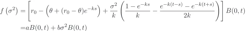
E[Ms] =P(0)
e−r0(T−s)+r
0(T−s)−1
r0(T −s) [1−e−r0T]
# T
s
$
r0−
dln(A1(s,t))
dt −
dln(A1(0,t))
dt +r0 dA2(0,t)
dt dA2(s,t)
dt
%
B(0, t)dt.
(3.11)
Lemma 3.2.3. If cs is defined as in(3.10), we have
cs> rs. (3.12)
Proof. We let x=rs(T −s), x0 =r0(T −s) , andy =cs(T−s). Thus, we have
g(x) = x0 1−e−x0 −
x
1−e−x.
Withg(x0) = 0 and g(0) = 1−xe0−x0 −1, the slopem is
m= g(0)−g(x0) 0−x0
= 1−e
−x0−x
0
(1−e−x0)x
0
.
Asg′(x)<0 and g′′(x)<0, there exists an uniquey∈(x, x0], such that
g(y) =m(x−x0),
Theorem 3.2.4. The optimal time to refinance, with ρ = 1, can be obtained by the following equation
(r0(T−s) + 1)e−r0(T−s)−1
(T−s)6
e−r0(T−s)+r0(T−s)−17
# T
s
$
r0−
dln(A1(s,t))
dt −
dln(A1(0,t))
dt +r0 dA2(0,t)
dt dA2(s,t)
dt
%
B(0, t)dt
=
; # T
s
∂2ln(A1(s,t))
∂s∂t
dA2(s,t)
dt −
∂2A2(s,t)
∂s∂t
2
dln(A1(s,t))
dt −
dln(A1(0,t))
dt +r0 dA2(0,t)
dt
3
2
dA2(s,t)
dt
32 B(0, t)dt
+
$
r0−
dln(A1(s,t))
dt |t=s−
dln(A1(0,t))
dt |t=s+r0 dA2(0,t)
dt |t=s dA2(s,t)
dt |t=s
%
B(0, s)
<
. (3.13)
In addition, we can obtain s by numerical methods.
Theorem 3.2.5. The analytical solution of E[Ms]is obtained whenct is a linear
func-tion of rt, say,ct=λrt, where λis a multiplier, with λ>1.
E[Ms] =
P(0) 1−e−λr0T
# T
s
λr0B(0, t)− 2
1−e−λr0(T−s)
35∞
n=0
Bn
(−1)nλn(T −s)n−1G(n)
α (0, s, t)
n! dt,
with G(α, s, t) = A1(s,t)
A1(s,˜t)B(0,
˜
t), and ˜t is a function of α and t. In addition, if α = 0, we have G(0, s, t) =B(0, t).
Lemma 3.2.6. With ct=λrt, Ms could be rewritten as
Ms=
P(0) 1−e−λr0T
# T
s
λr0e−
!t
0rvdv−
2
1−e−λr0(T−s)3
∞ 5
n=0
Bn
(−1)n(T−s)n−1
n! λ
nrn se−
!t
0rvdvdt,
(3.14)
whereBn is the sequence of Bernoulli numbers with the explicit formula
Bn= n 5 k=0 k 5 v=0
(−1)v
!
k v
"
(v+ 1)n
k+ 1 .
Proof. We may arrange Ms as
Ms=P(0)
$
c0
1−e−c0T −
cs
6
1−e−c0(T−s)7
[1−e−c0T]61−e−cs(T−s)7
% # T
s
e−!0trvdvdt
= P(0)
1−e−c0T
# T
s
c0e−
!t
0rvdv−1−e
−c0(T−s)
T−s
cs(T −s)
1−e−cs(T−s)e
−!t
0rvdvdt,
As we have
cs(T −s)
1−e−cs(T−s) =
∞ 5
n=0
Bn
(−1)n(T−s)ncn s
n! =
∞ 5
n=0
Bn
(−1)n(T −s)nλnrn s
thus, we may rewriteMs as
Ms=
P(0) 1−e−λr0T
# T
s
λr0e−
!t
0rvdv−
2
1−e−λr0(T−s)3
∞ 5
n=0
Bn
(−1)n(T−s)n−1
n! λ
nrn se−
!t
0rvdvdt.
Lemma 3.2.7. Assume ct=λrt. Then the asymptotic formula of (3.9) can be
simpli-fied as
Ms ≈λP(0)
1−e−λr0(T−s)−λr
0(T−s)e−λr0(T−s) 6
1−e−λr0(T−s)7[1−e−λr0T]
# T
s
(r0−rs)e−
!t
0rvdvdt, (3.15)
thus, the expectation of (3.15) is
E[Ms]≈λP(0)
1−e−λr0(T−s)−λr
0(T −s)e−λr0(T−s) 6
1−e−λr0(T−s)7[1−e−λr0T]
# T
s
$
r0−
dln(A1(s,t))
dt −
dln(A1(0,t))
dt +r0 dA2(0,t)
dt dA2(s,t)
dt
%
B(0, t)dt. (3.16)
Lemma 3.2.8. The approximation of c0
1−e−c0(T−s) −
cs
1−e−cs(T−s) is
c0
1−e−c0(T−s) −
cs
1−e−cs(T−s) ≈
1−e−c0(T−s)−c
0(T −s)e−c0(T−s) 6
1−e−c0(T−s)72
(c0−cs)
=λ1−e
−λr0(T−s)−λr
0(T −s)e−λr0(T−s) 6
1−e−λr0(T−s)72
(r0−rs).
However, the approximated value of Ms is slightly higher than the real value,
sug-gesting that our approximation will benefit the debtors. In this approximation method, the lender may charge for a higher transaction cost (with the higher value ofβ) to keep balance.
Proof. We let x = cs(T −s), x0 = c0(T −s) . As ∃ A, such that 0 ≤ x ≤ A, we
approximatef(x) = 1−xe−x −
x0
1−e−x0 at the pointx0 as
x
1−e−x −
x0
1−e−x0 =
1−e−x0 −x
0e−x0
[1−e−x0]2 (x−x0) +o(x−x0).
As
f′′(x) = −2e
−x+ 2e−2x+xe−x+xe−2x
[1−e−x]3 >0,
it is clear thatf(x) is a convex function, implyingo(cs−c0)>0.
Lemma 3.2.9. For any given function g(rs), we have
E2g(rs)rse−
!t
0rvdv
3
=−AdA1(s, t)
2(s,t)
dt
d dt
!
1
A1(s, t)
E2g(rs)e−
!t
0rvdv
3"
Proof.
E2g(rs)e−
!t
0rvdv
3
=E2E2g(rs)e−
!t
0rvdv|r
s
33
=E2g(rs)e−
!s
0 rvdvE
2
e−
!t srvdv|r
s
33
=E2g(rs)e−
!s
0 rvdvB(s, t)
3
=E2g(rs)e−
!s
0 rvdvA1(s, t)e−A2(s,t)rs
3
.
Taking derivative of both sides with respect tot gives
d dtE
2
g(rs)e−
!t
0rvdv
3
=E
&
g(rs)e−
!s
0 rvdvdA1(s, t)
dt e
−A2(s,t)rs
'
−E
&
g(rs)e−
!s
0rvdvdA2(s, t)
dt rsA1(s, t)e
−A2(s,t)rs
'
=dln [A1(s, t)]
dt E
2
g(rs)e−
!s
0 rvdvB(s, t)3− dA2(s, t)
dt E
2
g(rs)rse−
!s
0 rvdvB(s, t)3 =dln [A1(s, t)]
dt E
2
g(rs)e−
!t
0rvdv
3
−dA2dt(s, t)E2g(rs)rse−
!t
0rvdv
3
.
Rearranging the above equation gives
E2g(rs)rse−
!t
0rvdv
3
=dA1
2(s,t)
dt
&
−dtdE2g(rs)e−
!t
0rvdv
3
+dln [A1(s, t)]
dt E
2
g(rs)e−
!t
0rvdv
3'
=−AdA1(s, t)
2(s,t)
dt
d dt
&
1
A1(s, t)
E2g(rs)e−
!t
0rvdv
3'
.
This proves the Lemma.
Lemma 3.2.10. For any α in the positive neighborhood (0,ϵ), if we let G(α, s, t) = E2eαrse−!0trvdv
3
, there exists ˜t= ˜t(α, t)∈[s, t), such that
G(α, s, t) = A1(s, t)
A1(s,t˜)
B(0,t˜). (3.17)
Then we have
E2rnse−!0trvdv
3
=G(αn)(0, s, t) = d
n
dαn|α=0
!
A1(s, t)
A1(s,˜t)B(0,˜t)
"
. (3.18)
Proof. We have
G(α, s, t) =E2g(rs)e−
!s
0 rvdvB(s, t)3 =E2eαrse−!0srvdvA
1(s, t)e−A2(s,t)rs 3
=E2e−
!s
0 rvdvA
1(s, t)e−(A2(s,t)−α)rs 3
asA2(s, t) is an increasing function with respect tot, there exists ˜t, such that
0≤A2(s, t)−α=A2(s,˜t), (3.19)
and we can solve ˜tbased on the function of A2(s, t). Thus, the above equation can be
continued as
=E2e−!0srvdvA1(s, t)e−A2(s,˜t)rs
3
=A1(s, t)
A1(s,˜t)E
2
e−!0srvdvA1(s,t˜)e−A2(s,˜t)rs
3
=A1(s, t)
A1(s,˜t)
E2e−!0srvdvB(s,˜t)3
=A1(s, t)
A1(s,˜t)B(0,˜t).
Both Lemma 3.2.9 and Lemma 3.2.10 can be used to calculate E2rnse−!0trvdv
3
based on affine Models. However, Lemma 3.2.10 is more applicable to analytical analysis, and Lemma 3.2.9 is more suitable for numerical iteration.
Corollary 3.2.11. The same formulation of E2rse−
!t
0rvdv
3
can be obtained both by
Lemma 3.2.9 and Lemma 3.2.10.
Proof. We first consider g(rs) = 1 in Lemma 3.2.9, where
E2rse−
!t
0rvdv
3
=−AdA1(s, t)
2(s,t)
dt
d dt
!
1
A1(s, t)
E2e−!0trvdv
3"
=−AdA1(s, t)
2(s,t)
dt
d dt
!
1
A1(s, t)
B(0, t)
"
= AdA1(s, t)
2(s,t)
dt
dA1(s,t)
dt B(0, t)− dB(0,t)
dt A1(s, t)
A21(s, t)
= dA1
2(s,t)
dt
dA1(s,t)
dt B(0, t)− dB(0,t)
dt A1(s, t)
A1(s, t)
.
As we have
dB(0, t)
dt = d
dtA1(0, t)e
−A2(0,t)r0
= dA1(0, t)
dt e
−A2(0,t)r0 −r
0
dA2(0, t)
dt A1(0, t)e
−A2(0,t)r0
= dA1(0, t)
dt
1
A1(0, t)
A1(0, t)e−A2(0,t)r0 −r0
dA2(0, t)
dt A1(0, t)e
−A2(0,t)r0
= dln (A1(0, t))
dt B(0, t)−r0
dA2(0, t)
![Figure 4.1 demonstrates the numerical value of E[Ms] under Merton model. We](https://thumb-us.123doks.com/thumbv2/123dok_us/8075669.227586/51.595.121.529.96.209/figure-demonstrates-numerical-value-e-ms-merton-model.webp)

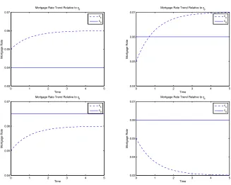
![Figure 4.1: The numerical value of E[MTs] under Merton model when T = 15 and = 30, where the value of the parameters are u = −0.001 and σ2 = 0.04.](https://thumb-us.123doks.com/thumbv2/123dok_us/8075669.227586/75.595.159.478.463.587/figure-numerical-value-mts-merton-model-value-parameters.webp)
![Figure 4.2: The numerical value of E[Ms] with different parameters under Vasicekmodel.](https://thumb-us.123doks.com/thumbv2/123dok_us/8075669.227586/76.595.154.481.439.691/figure-numerical-value-e-ms-dierent-parameters-vasicekmodel.webp)
![Figure 4.7: The numerical value of E[Ms] through different approximating methodsunder CIR model.](https://thumb-us.123doks.com/thumbv2/123dok_us/8075669.227586/78.595.151.482.100.349/figure-numerical-value-dierent-approximating-methodsunder-cir-model.webp)