Disappointment Aversion
Thesis submitted in accordance with the requirements of
the University of Liverpool for
the degree of Doctor in Philosophy
by
YUXIN XIE
ii
Abstract
The present thesis examines one of the non–standard preferences, the theory of disappointment aversion (DA) from Gul (1991), within an asset allocation problem. Related to the area of decision–making under risk, it sheds light on: (i) at the global level, how the risk exposure reduces quantitatively in the presence of disappointment aversion; (ii) given the empirical data, what are the plausible levels of disappointment aversion around different financial markets; and (iii) how disappointment aversion interacts with both inherent risk attitudes (i.e., risk aversion, subjective probability weighting and cultural dimensions) and environmental stimuli (i.e., pleasant or unpleasant odours).
In Chapter 2, drawing upon the seminal study of Ang et al. (2005), we incorporate disappointment aversion (that is, extra aversion to outcomes that are worse than prior expectations) within a simple theoretical portfolio choice model. Based on the results of this model, we then empirically address the portfolio allocation problem of an investor who chooses between a risky and a risk–free asset using international data from 19 countries. Our findings strongly support the view that disappointment aversion leads investors to reduce their exposure to the stock market (i.e., disappointment aversion significantly depresses the portfolio weights on equities in all cases considered). Overall, our study shows that, in addition to risk aversion, disappointment aversion plays an important role in explaining the equity premium puzzle around the world.
In Chapter 3, we investigate investors’ asset allocation when their utility consists of wealth utility and disappointment aversion utility in which gains and losses are calculated with respect to the expected wealth. We show that optimal investment proportions increase when disappointment aversion on the assets decreases, and that disappointment aversion increases when expected excess returns increase. When decreasing absolute risk aversion holds, disappointment aversion increase with wealth, which is supported by our empirical results with asset allocations in pension funds of 35 OECD countries. We also find that individualism is positively related to disappointment aversion. These results indicate that the overconfidence represented by their individualism leads to more disappointment when losses occur.
Chapter 4 aims to investigate the role of odours on DA in a monetary gamble task. We elicited the degree of DA based on an experimental procedure similar to Sokol-Hessner et al. (2009, 2013). Our study shows for the first time that unpleasant odours increase DA in a monetary gamble task. Such odour–related variations in individual DA were associated with hedonic evaluations of odours but not with odour intensity. Increased disappointment aversion while perceiving an unpleasant odour suggests a dynamic adjustment of aversion to losses. Given that odours are biological signals of hazards, such adjustment of disappointment aversion may have adaptive value in situations entailing threat or danger.
Contents
Preface v
Acknowledgement vii
List of Tables viii
List of Figures ix
1 Introduction 1
1.1 General Introduction . . . 3
1.1.1 The Equity Premium Puzzle . . . 4
1.1.2 The Preference of Loss Aversion and Probability Weighting . 5 1.1.3 Gul’s Theory of Disappointment Aversion . . . 7
1.2 Contributions and Structure . . . 10
1.3 Tables & Figures of This Chapter . . . 13
2 Disappointment Aversion and the Equity Premium Puzzle: New International Evidence 15 2.1 Introduction . . . 17
2.2 The Disappointment Aversion Asset Allocation Framework . . . 19
2.3 Data and Descriptive Statistics . . . 21
2.4 Empirical Results . . . 23
2.4.1 Replicating the Optimal Portfolio Weights of Ang et al. (2005) 23 2.4.2 Optimal Portfolio Weights . . . 24
2.5 Conclusion . . . 27
2.6 Tables & Figures of This Chapter . . . 29
3 A Cross–Cultural Study of Financial Risk–Taking: Individualism and Disappointment Aversion around the World 43 3.1 Introduction . . . 45
3.2 Disappointment Aversion in Asset Allocation . . . 47
3.2.1 The Disappointment Aversion Utility . . . 48
iv CONTENTS
3.2.3 An Application to an Asset Allocation Problem . . . 51
3.2.4 Disappointment Aversion and Individualism . . . 56
3.3 Empirical Tests . . . 57
3.3.1 Asset allocation and Returns across Countries . . . 57
3.3.2 Individualism and Risk Aversion . . . 61
3.3.3 Cross–Country Disappointment Aversion . . . 63
3.3.4 Individualism vs. Disappointment Aversion . . . 64
3.3.5 Robustness Tests . . . 66
3.4 Discussion and Conclusion . . . 68
3.5 Tables & Figures of This Chapter . . . 70
4 Dynamic Disappointment Aversion in Different Odours: An Experimental Study 86 4.1 Introduction . . . 88
4.2 Methods . . . 89
4.2.1 Subjects . . . 89
4.2.2 Procedure . . . 90
4.2.3 Monetary Gamble Task . . . 91
4.2.4 Eliciting Disappointment Aversion . . . 92
4.3 Results . . . 95
4.3.1 Odour Ratings . . . 95
4.3.2 Odours and Disappointment Aversion . . . 96
4.4 Discussion and Conclusion . . . 98
4.5 Tables & Figures of This Chapter . . . 99
5 Conclusion and Further Directions 108 5.1 General Conclusion . . . 110
5.2 Further Directions . . . 112
A Appendix 116
B Appendix 118
Preface
Elements of this thesis have appeared in the following publications:
Journal Papers:
Xie, Y., Pantelous, A.A. and Florackis, C. (2014) ‘Disappointment aversion and the equity premium puzzle: new international evidence.’ The European journal of finance(page forthcoming).
Xie, Y and Pantelous, A.A. (2014) ‘Asset allocation with disappointment aversion.’
ASCE–ASME proceedings: vulnerability, uncertainty, and risk: quantification,
mitigation, and management: pp. 1180–1189.
Stancak, A., Xie, Y., Fallon, N., (Bulsing, P.), (Giesbrecht, T.), (Thomas, A.), Pantelous, A.A. (2014) ‘Unpleasant odors increase loss aversion in a monetary gamble task.’ Biological Psychology(minor revision).
Hwang, S., Pantelous, A.A., Xie, Y. (2014) ‘A cross–cultural study of financial risk–taking: individualism and disappointment aversion around the world.’ (To be submitted toJournal of Financial and Quantitative Analysis.)
Refereed Conferences:
ASCE–ICVRAM–ISUMA Conference Liverpool, UK
Hwang, S., Pantelous, A.A., Xie, Y. (2014) ‘A cross–cultural study of financial risk–taking: individualism and disappointment aversion around the world.’
Acknowledgements
If there is something I have learned from this research during my Ph.D., it has to be the persistence to deal with failures. I will not forget: those days and nights I was struggling to model an idea, solve an equation or debug several lines of code. I will not forget those days and nights I made things right as the result of my countless attempts. Some say our potential mostly depends on talent; I say that according to my experiences, the attitude, the way we do things makes all the difference.
My supervisor, Associate Professor Athanasios A. Pantelous, deserves a special mention in these acknowledgements. He believed and supported my ideas from the very first day. His deep knowledge and critical thinking have been a constant source to inspire me and guide me in the right direction. His utmost patience, encouragement and sense of humour during many difficult moments have been invaluable to me. He has taught me much more than doing research itself, which is certainly beyond his responsibility. Dear Thanasi, thanks a lot for your care! I am also very grateful to my second supervisor, Associate Professor Chris Florackis, who has taught me about many financial tools and spent an enormous time reading and editing my draft. The presented work benefited a lot from his honest and in–depth feedback. His professional accomplishment has been fundamental to my progress.
I am eternally grateful to my parents for their constant support since I was born. The help (both financial and psychological) you have given me to achieve as much as I could is the reason I have managed to go so far and I am indebted to you for being there whenever I needed you. I would like to thank my wife as well, who had been always supportive of my study abroad. I know you have sacrificed a lot owing to my absence so far but you are essential to my future life.
viii LIST OF TABLES
List of Tables
1.1 Equity Premium in Selected Countries . . . 13
2.1 Descriptive Statistics of Worldwide Equity Premiums . . . 29
2.2 S&P 500 and Treasury Bill Returns from CRSP . . . 30
2.3 Replicating the Optimal Weights of Ang et al. (2005) . . . 31
2.4 Optimal Portfolio Weights under Different A Values . . . 32
3.1 Asset Allocations of Pension Funds . . . 70
3.2 Summary Statistics of Asset Returns . . . 72
3.3 Hofstede’s Uncertainty Avoidance Index around the World . . . 73
3.4 Hofstede’s Individualism Index around the World . . . 74
3.5 Disappointment Aversion over Different Assets . . . 75
3.6 Regression Results . . . 78
3.7 Disappointment Aversion under Different Risk–Related Parameters 81 3.8 Robustness Tests under Different Degrees of Probability Weighting . 84 4.1 List of Risky Gains and Assured Wins Used in the Experiment . . . 99
4.2 Estimations of Disappointment Aversion, Risk Aversion and Logit Sensitivity . . . 100
4.3 Means of Disappointment Aversion over Three Odours . . . 103
4.4 One–Way Repeated Measures ANOVA between Disappointment Aversion and Different Odours . . . 104
List of Figures
Chapter 1
1.1 General Introduction
The traditional finance paradigm relies heavily on an assumption of “fully rational agents”. In the field of finance, the concept “rational” typically means two things: (i) people evaluate risk and make decisions based on the expected utility of Von Neumann and Morgenstern (1944), where their preferences are complete, continuing, transferable and independent across states; (ii) new information will be updated into their beliefs in the manner of Bayes’ rules. Such settings make the traditional framework appealingly predictable because agents always make consistent choices to maximize their expected utility. However, recent facts about the cross section of average returns (i.e., equity premium puzzle (Mehra and Prescott, 1985; Mehra, 2008)) and inconsistencies of observed choice data (Allais, 1953; Ellsberg, 1961; Tversky and Kahneman, 1974) have promoted a rethink of investors’ behaviour in terms of decision–making under risk. After years of effort, there has been an explosion of progress on so–called non–expected utility theories (Loomes and Sugden, 1982; Bell, 1985; Gul, 1991; Segal, 1987, 1989; Quiggin, 1982; Tversky and Kahneman, 1974) which makes it even clearer that people violate the assumption of expected utility theory when assessing risk.
During the early 1980s, behavioural finance eventually emerged, at least in part, in response to the financial anomalies that cannot be fully understood by traditional frameworks. Generally speaking, it argues that investors are not fully rational agents. Specifically, it investigates whether better explanations can be achieved by using a non–standard preference (i.e., situations where people do not evaluate risk according to the expected utility) and non–standard beliefs (i.e., situations where people’s beliefs are subject to psychological biases and deviate from Bayes’ law).
4 1.1 General Introduction
aversion in prospect theory (Tversky and Kahneman, 1979, 1992). Moreover, a novel framework has been developed to estimate aggregate disappointment aversion quantitatively around different financial markets. We then analytically show how the disappointment aversion is related to other factors such as risk aversion and cultural variations. In addition to economic attributes, an experimental procedure is conducted to explore whether disappointment preferences are affected by external stimuli (i.e., pleasant & unpleasant odours). We use a few subsections below to briefly discuss the key concepts in this study.
1.1.1 The Equity Premium Puzzle
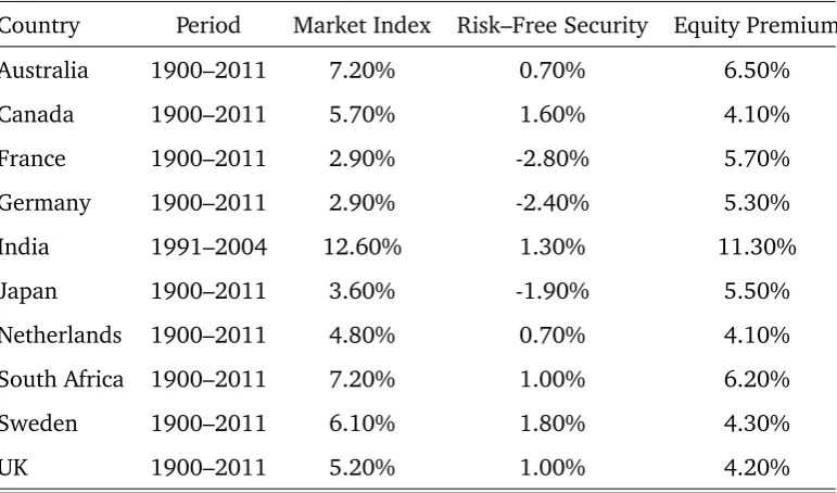
It stands to reason that equities should earn higher returns than risk–free assets in the long run. However, how can we know the historical equity premiums are at a reasonable level? Using Lucas’s (1978) standard general equilibrium model, Mehra and Prescott (1985) firstly document how the required equity premium in the American market is only about 0.35%, which is inconsistent with the observed premium of 6.18%. Similar statistical differentials are documented for Australia, Canada, France, Germany, India, Japan, the Netherlands, South Africa, Sweden, and the UK (Dimson et al., 2008; Mehra, 2007). Table 1.1 lists the equity premiums for these countries.
[Insert TABLE 1.1 about here]
The equity premium puzzle arises as solely relying on risk aversion fails to explain the huge magnitude of equity premium. In order to necessarily match the observed equity premiums, risk aversion should reconcile itself to a value from 30 to 40, which Mehra and Prescott conclude is too high to be plausible. To put it another way, even though stocks are more attractive than relatively risk–free assets, investors appear to be so unwilling to hold stocks that they demand a substantial risk premium in order to hold the market supply.
categories. Either the existing data misdirected the problem to statistical illusions (empirical side) or else current models were short of responses to potential factors (theoretical side). On the empirical side, the existence of the puzzle has been questioned by several researchers who interpret the “abnormal” stock returns as a statistical illusion driven by common biases (e.g., survivorship, success and selection bias) or the use of non–stationary data (Fama and French, 2002; Dimson and Staunton, 2006). On the theoretical side, various risk–related explanations that have been proposed to stress the inability of the standard risk paradigm are: the risk–free rate puzzle (Weil, 1989); non–time separable utility (Epstein and Zin, 1991); economic catastrophe concerns (Barro, 2006); idiosyncratic and uninsurable income risk (Constantinides and Duffie, 1996); and habit formation (Constantinides, 1990; Abel, 1990; Campbell and Cochrane, 1999; Campbell, 2001).
1.1.2 The Preference of Loss Aversion and Probability Weighting
Instead of being “fully rational” during the decision–making process, a common question is: what is the best plausible alternative to describe how people think about risk? A famous answer from the behavioural perspective is the prospect theory of Tversky and Kahneman (1979, 1992). Fundamental to prospect theory is the preference of loss aversion, which suggests that (i) decisions are made according to the potential losses and gains rather than final wealth; (ii) agents evaluate potential outcomes based on a reference point; and (iii) the utility is steeper in losses than gains of the same magnitude. Formally, a value function with loss aversion can be shown in the following form:
U(x) =
xv+, x≥0 −λ(−x)v−, x <0,
whereλis the coefficient that controls the degree of loss aversion,v+ andv−
6 1.1 General Introduction
Among many subsequent studies, the idea of loss aversion has been particularly successful in explaining the equity premium puzzle (i.e., Benartzi and Thaler, 1995; Barberis et al., 2001; Hwang and Satchell, 2010). The simple logic is that: as people are loss–averse, if stock market goes up in the next year, they will feel good; on the other hand, if the stock returns lead to losses in the next year, they will feel verybad. As a result of this kind of thinking, in addition to risk aversion, investors tend to consider stocks less favourably and require an extra premium in order to keep their holdings.
The concept of probability weighting is proposed in dealing with choice inconsistencies documented in subsequent research of prospect theory. As relying on only the objective probability weighting function is not sufficient to match the complexity of behavioural patterns observed in experimental investigations, people tend to overweight unlikely extreme outcomes. Quiggin (1982) introduces a rank–dependent utility model where weights depend on the true probability of an outcome as well as its ranking relative to other outcomes. The combination of rank and reference point dependent utility gives birth to a later version of prospect theory, the cumulative prospect theory (CPT) of Tversky and Kahneman (1992). CPT utilizes a transformed probability weighting function to account for the redistribution of decision weights that overweight small probabilities and underweight moderate and high probabilities. In particular, it is defined for gains and losses separately:
w+(p) = p
γ+
pγ+
+ (1−p)γ+ 1
γ+
, w−(p) = p
γ−
pγ−
+ (1−p)γ− 1
γ−
,
where p is the cumulative probability of any possible outcome. With one extra curvature parameter γ (0< γ <1,γ+ for gains andγ−for losses), the weighting function allocates more (less) weight to unlikely (likely) events. In other words, tails of any distribution are over–emphasized while those outcomes around its peak are less valued.
parameter is identical for both the domains of losses and gains. This simplifies the function to:
w(p) =exp[−(ln(p))γ].
According to the experimental work of Gonzalez and Wu (1999), despite its simplicity, the use of symmetric curvature fits the median data as well as the other separate–curvature models. Therefore, for the numerical investigations in Chapter 3, we use Prelec’s weighting functions as our primary setting. For a demonstration here; suppose a stock has normally distributed annual returns with µr = 10%,
standard deviation=0.1865, and letδ = 0.741. Figure 1.1 compares the CPT and Prelec’s weighting functions to its original density function.
[Insert FIGURE 1.1 about here]
A glance at Figure 1.1 shows important attributes of the weighting function. Firstly, decision weights are underweighted for the region of more frequent events. As now small gains become less attractive, investors are less motivated to take further risks. On the contrary, fewer decision weights on tiny losses ease the panic of suffering. Investors therefore have a higher tendency to play with risks. Secondly, decision weights are exaggerated at the edges of the distribution. Investors become risk–seeking if they recognize a massive gain possibility, even if the chance of occurrence is small. On the other hand, additional concerns about those very unlikely huge losses make investors extremely safety–oriented, as now, in their view, a disaster–like outcome occupies more decision weight than it should do. Lastly, the modified density functions are highly non–linear, resulting in more severe sensitivity nearp= 1, andp= 0.
1.1.3 Gul’s Theory of Disappointment Aversion
The term “disappointment” was first used by Bell (1985) within the context of binary lotteries. According to Bell, disappointment is a psychological reaction to an outcome that fails to satisfy expectations held by the decision–maker. Consider
1Analogous to the estimation of Gonzalez and Wu (1999), in the rest of this study,δ = 0.74is
8 1.1 General Introduction
a lottery(x, p, y), which has a probabilitypof winningxand a probability(1−p) of yieldingy,(x > y). The decision–maker’s expectation depends on the expected pay–off of this lottery: c=px+ (1−p)y.
The decision–maker will be disappointed if y occurs, which means he/she receives less than expected; the measure of such disappointment is:
d(c−y) =d(px+ (1−p)y−y) =dp(x−y).
On the contrary, the outcome will be regarded as “elation” ifxis received:
e(x−c) =e(x−px−(1−p)y) =e(1−p)(x−y),
where d (e) (d ≥ 0, e ≥ 0) controls the proportional disappointment (elation) between the realised outcomes and expectations. The net psychological satisfaction that comes with the lottery can be expressed as:
p(e(x−c))−(1−p)(d(c−y)) = (e−d)p(1−p)(x−y).
Finally, the overall utility function is based on the expected economic pay–off (consumption) and her/his psychological satisfaction:
U(·) = [px−(1−p)y] + (e−d)p(1−p)(x−y).
Although Bell’s model has intuitive appeal, it is restricted to binary lotteries only. Following his idea, Gul (1991) proposed the theory of disappointment aversion (DA) that is more general in describing decision–making under risk. At the core of Gul’s framework, potential outcomes are further divided into elation and disappointment based on an endogenous reference point. People are supposed to be disappointment–averse: they are more sensitive to disappointment than elation of the same magnitude. Consider the following piecewise utility as a compact way to show the functional form of disappointment aversion:
U(x) =
xt+h−Etxt+h
, xt+h ≥Etxt+h
A xt+h−Etxt+h
, xt+h <Etxt+h
Let h be the investment horizon while Etxt+h refers to the applicable reference
point that all outcomes duringt+hwill be compared with. The level ofEtxt+his
determined by the certainty equivalent (the certain level of wealth that generates the same utility according to an investor’s choices). Such a prospect–dependent feature means the reference point does not necessarily have to be positive when the market outlook turns stagnant. Additionally, Routledge and Zin (2010) allow the reference point to lie below the certainty equivalent. However, we maintain the scope of this study within the case where the reference point is equal to the certainty equivalent. With only one parameter richer than the expected utility,A
10 1.2 Contributions and Structure
1.2 Contributions and Structure
In the literature, the preference of disappointment aversion only appears in equilibrium models over consumption (Epstein and Zin, 1990, 2001). Within this thesis, we embed disappointment aversion into a typical asset allocation problem. In broad terms, we argue that the portfolio choices between risky assets and risk– free assets are jointly determined by risk aversion and disappointment aversion. In Chapter 2, by extending the seminal study of Ang et al. (2005) to the global scale, we have demonstrated to what extent the equity weights will drop in response to the presence of disappointment aversion among 19 different markets. With a sufficient level of disappointment aversion, investors may not even participate in the equity market.
preferences also depend on absolute consumption levels. In line with Koszegi and Rabin (2007), we define the basic form of utility in Chapter 3, where the overall utility has two components: U(c|r) = m(c) +n(c|r), m(c) is a “consumption utility” typically stressed in economics and n(c|r) is an “elation–disappointment utility” generated from risk–taking activities in terms of a reference pointr.
From the empirical side, results in Chapter 3 argue that cultural differences can play an important role during the decision–making process under risk, which is consistent with the view that investors from different backgrounds frame their risk attitude in different ways and are subject to psychological biases (e.g., Chui et al., 2010; Beugelsdijk and Frijns, 2010; Frijns et al., 2013; Breuer et al., 2014). The cultural variation of DA challenges the traditional risk–based theories and contributes a new dimension to current behavioural literature. Additionally, consistent results are also found to support the assertion that investors tend to apply different rules to decide their holdings instead of assessing them as a portfolio. This tendency is classified asnarrow framing, which is another popular idea among the behavioural studies (e.g., Berkelaar et al., 2004; Gomes, 2005; Barberis et al., 2006; Barberis and Huang, 2009).
Chapter 4 aims to investigate the impact of environmental stimuli (pleasant & unpleasant odours) on DA in a monetary gamble task. We elicited the level of DA based on an experimental procedure similar to Sokol-Hessner et al. (2009, 2013). Our study shows for the first time that unpleasant odours increase DA in a monetary gamble task. Odour–related individual variations in DA were associated with hedonic evaluations of odours but not with odour intensity. Increased disappointment aversion while perceiving an unpleasant odour suggests a dynamic adjustment of aversion towards greater sensitivity to losses. Given that odours are biological signals of hazards, such adjustment of disappointment aversion may have adaptive value in situations entailing threat or danger.
12 1.2 Contributions and Structure
1.3 Tables & Figures of This Chapter
Table 1.1
Equity Premium in Selected Countries
This table presents real mean returns in selected countries. All data except India are sourced from the Global Investment Returns Yearbook 2012 distributed by
Morningstar; data in India’s refer to Mehra (2007).
Country Period Market Index Risk–Free Security Equity Premium
Australia 1900–2011 7.20% 0.70% 6.50%
Canada 1900–2011 5.70% 1.60% 4.10%
France 1900–2011 2.90% -2.80% 5.70%
Germany 1900–2011 2.90% -2.40% 5.30%
India 1991–2004 12.60% 1.30% 11.30%
Japan 1900–2011 3.60% -1.90% 5.50%
Netherlands 1900–2011 4.80% 0.70% 4.10%
South Africa 1900–2011 7.20% 1.00% 6.20%
Sweden 1900–2011 6.10% 1.80% 4.30%
14 1.3 Tables & Figures of This Chapter
Figure 1.1
Probability Weighting Function vs. Original Density Function
This figure compares the KT’s (Kahneman and Tversky) and Prelec’s weighting functions to its original density function. The stock returns are supposed to follow a normal distribution with moments: µr= 10%,standarddeviation= 0.1865, and
Chapter 2
Disappointment Aversion and the
Equity Premium Puzzle: New
2.1 Introduction
A number of studies have shown that stocks outperform bonds over long horizons by a surprisingly large margin. For example, Mehra and Prescott (1985) report that the annual real return on the US stock market has exceeded that of bonds by about 6.36% over the last 116 years. This empirical regularity, commonly referred to as the “equity premium puzzle”, is not unique to the US market but is also observed in other international markets. Dimson and Staunton (2006) and Mehra (2007) report a significant equity premium for several developed (e.g., UK–6.1%; Australia–8.5%; Germany–9.1%; Japan–9.8%) and developing markets (e.g., India–11.3%).
A large volume of empirical and theoretical research focuses on the origin and the drivers of the equity premium puzzle2. On the empirical side, the existence of a puzzle has been questioned by several researchers who interpret the “abnormal” stock returns as a statistical illusion driven by common biases (e.g., survivorship, success and selection bias) or the use of non–stationary data (Fama and French, 2002; Dimson and Staunton, 2006). On the theoretical side, various risk–related explanations have been proposed to stress the inadequacy of the standard risk paradigm: the risk–free rate puzzle (Weil, 1989); non–time–separable utility (Epstein and Zin, 1991); economic catastrophe concerns (Barro, 2006); idiosyncratic and uninsurable income risk (Constantinides and Duffie, 1996); and habit formation (Constantinides, 1990; Abel, 1990; Campbell and Cochrane, 1999; Campbell, 2001).
Behavioural finance has emerged in response to the failure of traditional models to fully explain investment behaviour. Its key assumption is that investors do not always make rational decisions (see Barberis and Thaler, 2003). Following a series of influential papers by Tversky and Kahneman (1974, 1979, 1992), a growing body of literature focuses on behavioural explanations of the equity premium puzzle. Fundamental to the prospect theory of Tversky and Kahneman (1979) is the concept of loss aversion, which refers to the tendency to
2DeLong and Magin (2009) and Mehra (2008) provide reviews on the equity premium puzzle
18 2.1 Introduction
prefer avoiding losses over acquiring gains. A similar, though not identical, concept of loss aversion is that of disappointment aversion. Gul (1991) develops an axiomatic disappointment aversion framework where agents form an endogenous expected certainty equivalent. Outcomes below that equivalent are treated as “disappointment”. Since the reference point of disappointment aversion could possibly be higher than the status quo, even positive outcomes that lie below the reference point may still disappoint investors. Preferences that express disappointment aversion and loss aversion share the following three features: i) reference dependence; ii) diminishing sensitivity; and iii) a steeper value function of negative utility. The main difference stems from the way in which the reference point is determined in each case. In the case of loss aversion, a pre–set exogenous reference point is frequently applied, e.g., the status quo
(see Tversky and Kahneman, 1979, 1992), and the risk–free rate (see Barberis and Huang, 2001; Barberis et al., 2001). In the case of disappointment aversion, the reference point is endogenously determined according to investors’ former expectations (see Gul, 1991). Such a prospect–dependent feature is known as the certainty equivalent3.
This study adopts a “behavioural” perspective and attempts to provide further insights into the drivers of the equity premium puzzle. In particular, drawing upon the portfolio choice model of Ang et al. (2005), we incorporate disappointment aversion within a simple theoretical asset allocation model. Based on the results of this model, we then empirically address the portfolio allocation problem of an investor who chooses between a risky and a risk–free asset. An important contribution is the international nature of our study. While Ang et al. (2005) focus exclusively on the US market over the period 1926–1998, our analysis is based on the Dimson–Marsh–Staunton (DMS) database distributed by Morningstar4, which contains data spanning 112 years of history
3The choice of an exogenous or endogenous reference point is particularly relevant in
applications that consider long investment horizons. For example (Fielding and Stracca, 2007), show that, under a fixed reference point, the loss aversion parameter is inflated to 25 at the 10–year horizon. In contrast, under a reference point that is endogenously determined, the disappointment aversion parameter only mildly increases to 2.5.
4Dimson et al. (2008) demonstrate that equity premiums around the world can be overstated due
across 19 countries and is free of ex–post selection bias. This is important because the magnitude of the equity premium differs significantly across markets (see Dimson and Staunton, 2006; Mehra, 2008). Extending the study of the equity premium puzzle to the global market helps to understand whether such differences can be attributed to behavioural or non–risk–based explanations (e.g., differences in borrowing constraints, transaction costs, etc.). To our knowledge, this is the first paper to examine whether disappointment aversion plays a role in explaining the international equity premium puzzle.
Our findings strongly confirm the view that disappointment aversion leads investors to reduce their exposure to the stock market (i.e., disappointment aversion significantly depresses the portfolio weights on equities in all cases considered). Our analysis also helps to determine the optimal weights between the risky and risk–free assets for each considered markets. The key result that emerges from our study is that optimal equity proportions around the world are jointly determined by the levels of risk and disappointment aversion. Taken together, these findings enhance our understanding of the sources of the international equity premium puzzle.
The remainder of this chapter is organized as follows: Section 3.2 presents a simple asset allocation framework under disappointment aversion, which draws upon Ang et al. (2005). Section 3.3 provides details about the dataset utilized and Section 3.4 presents our results. Finally, Section 3.5 concludes this chapter.
2.2 The Disappointment Aversion Asset Allocation Framework
This section presents the classical asset allocation framework under preferences that exhibit disappointment aversion (see Gul, 1991; Ang et al., 2005). Drawing upon Ang et al. (2005), the utility maximization problem can be
20 2.2 The Disappointment Aversion Asset Allocation Framework
expressed as follows:
max
α∈[0,1]U(µw). (2.1)
The DA utility is defined by
U(µw) = µw
R
−∞
U(W)dF(W) +A ∞
R µw
U(W)dF(W)
P r(W ≤µw) +AP r(W > µw)
, (2.2)
where µw refers to the certain level of wealth that generates the same utility
determined by the optimal weights to equities. This is referred to as the certainty equivalent. U(·)is the CRRA power utility in the form ofU(W) = W1−γ/(1−γ)
5;Ais the coefficient of disappointment aversion (where0< A <16). F(·)is the
cumulative distribution function for wealth W. The first–order condition (FOC) for the DA investor is given by the following expression:
E
∂U(W)
∂W (exp(y)−exp(r))1W≤µw
+AE
∂U(W)
∂W (exp(y)−exp(r))1W >µw
,
(2.3) where1is an indicator function andErefers to the expected value of the certainty
equivalent. According to Eq. (2.3) above, the DA utility function only concentrates on the differentiation between terminal wealth levels andµw, and neither previous
losses nor gains will be taken into account directly. Letαrepresent the proportion of equity investment. The ending period wealth (denoted by W) is defined as follows:
W =αW0(exp(y)−exp(r)) +W0exp(r). (2.4)
In this framework, the investor chooses between the risky assety(i.e., equity) and the risk–free asset r (i.e., Treasury bills). The termα refers to the proportion of wealth invested in the risky asset whileα∗ is the optimal weight. Ifµw is known,
5Using different forms of utility, empirical studies with similar preferences find consistent results.
For instance, within a classical power function, Barberis and Huang (2001) report a positive link between loss aversion and stock returns. Similarly, by utilising a standardized two–piece power function, Hwang and Satchell (2010) find a negative relationship between stock holdings and loss aversion.
6To ease the comparison with Ang et al. (2005), the coefficient
α∗ can be calculated by solving Eq. (2.3). The tricky part is that µw is also a
function of α, which means that a system of simultaneous equations has to be solved (Eqs. (2.2) and (2.3)). In this study, we develop an algorithm of numerical quadrature which converts Eqs. (2.2) and (2.3) into the following form7:
µ1w−γ =
P s:Ws≤µw
psWs1−γ+A P s:Ws>µw
psWs1−γ
P r(W ≤µw) +AP r(W > µw)
, (2.5)
X s:Ws≤µw
psWs−γ(exp(ys)−exp(r))+A X s:Ws>µw
psWs−γ(exp(ys)−exp(r)) = 0. (2.6)
Using Eqs. (2.5) and (2.6), one can solve the optimal asset allocation problem and determine theα∗. This can be done using a series of bisection searches to identify the correct excess return interval and as a result determine the optimal weights8.
Solving the system above provides optimal weights that usually lie between the interval [0, 1]. A value ofα∗that equals 0 implies that the optimal portfolio choice includes no exposure to the equity market (i.e., risky asset). A value of α∗ that equals 1 implies that all wealth is invested in equities. Our model is not restricted to producing weights only within the [0, 1] interval. A negative weight implies that investors anticipate under performance of the equity market, leading them to take short (optimal) positions on equities. On the contrary, a weight greater than 1 indicates that the optimal strategy involves borrowing for the purchase of equity. As shown in Section 4.1, our algorithm produces optimal weights that are similar to those obtained by Ang et al. (2005) in the case of the US market. The aim of this chapter is to extend their framework to an international context and examine the role of disappointment aversion in the equity premium puzzle around the world.
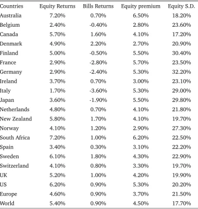
2.3 Data and Descriptive Statistics
For the empirical analysis, we use the Dimson–Marsh–Staunton (DMS) database distributed byMorningstar. The main advantage of this database is that it is free of ex–post selection bias, a common problem in the empirical literature
7See Appendix for details.
22 2.3 Data and Descriptive Statistics
on the equity premium puzzle. Our final sample is obtained by the 2012 Global Investment Returns Yearbook9 and contains data spanning 112 years of history
(from 1900 to 2011) across 19 countries: Australia, Belgium, Canada, Denmark, Finland, France, Germany, Ireland, Italy, Japan, the Netherlands, New Zealand, Norway, South Africa, Spain, Sweden, Switzerland, the UK and the US. Our final sample comprises more than 85% of total market capitalization around the world. In addition to the DMS database, we use return data from the Center for Research in Security Prices (CRSP) in order to replicate the findings of Ang et al. (2005) for the US market (see Section 2.4.1 for details). The main stock market index in each case represents investments in the risky asset. For the risk–free benchmark, we focus on T–bills issued in each country10.
Table 2.1 presents some descriptive statistics of our data. The equity premium lies between 2.80% in Belgium and 6.50% in Australia. The annual equity return on the US (UK) stock market is 6.20% (5.20%); this represents a notable 5.30% (4.20%) premium over the US (UK) bills returns. At a global and European level, the out performance of stocks over T–bills is 4.50% and 3.70%, respectively.
An interesting finding that emerges from Table 2.1 is that higher returns are not always associated with higher volatilities (e.g., the highest volatility observed in the German stock market (at 32.20%) is associated with one of the lowest equity returns (at 2.90%)). One potential explanation is the following. Classic asset pricing models such as the capital asset pricing model (CAPM) of Sharpe (1964) and Lintner (1965) suggest that higher volatilities command higher equity premiums. However, the empirical evidence on the relationship between risk and return is still mixed and inconclusive. While a significant body of research supports the traditional positive return–risk trade–off (e.g., see Bollerslev et al., 1988; Harvey, 1989; Ghysels et al., 2005), another strand in the literature reports results that reject this view (e.g., see Campbell, 1987; Breen
9See Credit Suisse: Global Investment Returns Yearbook 2012. This report is associated with
the work of Elroy Dimson, Paul Marsh and Mike Staunton, whose book Triumph of the Optimists (Princeton University Press, 2002) has had a major influence on investment analysis.
10Short–term T–bills (Treasury bills) are often backed by government finance which immunizes
et al., 1989). A third group of studies further suggests that the relation between risk and return is time–varying (e.g., see French et al., 1987; Campbell and Hentschel, 1992). We argue that one needs to go beyond risk aversion to fully understand the nature of the risk–return trade–off. Put differently, investors are not only concerned about volatility when making investment decisions, but also about the frequency of outcomes that are worse than prior expectations. In what follows, we demonstrate that, in addition to risk aversion, disappointment aversion significantly suppresses equity holdings (i.e., investments in the risky asset). In this way, our findings provide useful insights into the ambiguous risk–return relationship.
[Insert TABLE 2.1 about here]
2.4 Empirical Results
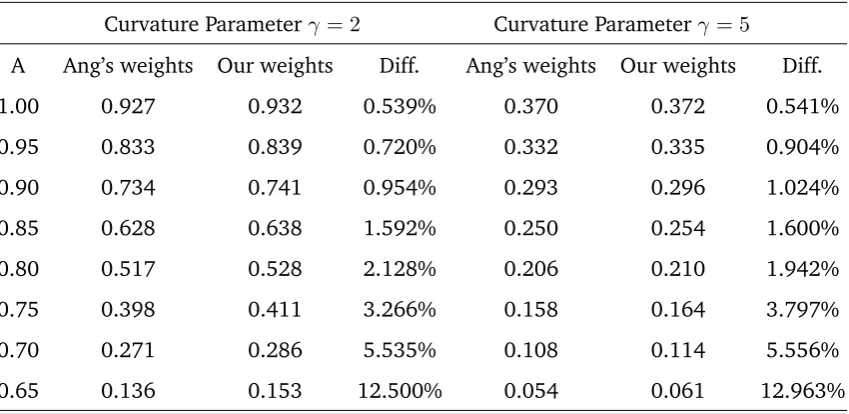
2.4.1 Replicating the Optimal Portfolio Weights of Ang et al. (2005)
Before presenting the optimal portfolio weights for the cases considered in our sample, we provide some preliminary evidence that confirms the validity of the algorithm used in our study to solve the portfolio choice problem. In particular, we try to replicate the optimal weights of Ang et al. (2005) for the case of the US market. Given that our DA framework embeds an endogenous certainty equivalent (see Gul, 1991; Ang et al., 2005), the impact of the rebalancing period becomes less of an issue (see Benartzi and Thaler, 1995; Fielding and Stracca, 2007). We therefore focus on overall sample means to calculate the optimal weights. Table 2.2 presents the summary statistics of the data used in order to conduct such an exercise. Over the 1926–1998 period, equities generated a nominal rate of return of 2.66% per quarter (10.64% annualized). Over the same period, the annual rate of return for T–bills was 4.08%. As expected, equities exhibited a much higher standard deviation compared to T–bills (21.94% vs. 1.72%).
24 2.4 Empirical Results
Table 2.3 presents the optimal weights produced from our algorithm and compares them with those reported in Ang et al. (2005). For ease of comparison, we present results for different levels of risk aversion (γ = 2 and γ = 5) and disappointment aversion (from 0.65, which represents a high DA aversion, to 1, which represents no DA aversion). Our optimal weights are very similar to those reported in Ang et al. (2005). Some differences across certain values ofAandγ
are due to differences in the investment horizon considered (horizon effect). The weight differences (Diff) is obtained using (our weights – Ang’s weights)/Ang’s weight. it tend to decrease as disappointment aversion declines, and essentially disappear in the case when there is no DA aversion (A = 1). The results also show that our weights are comparable to the ones in Ang et al. (2005) for different levels of risk aversion(γ = 2andγ = 5). Finally, it is interesting to note our A∗ value (i.e., the lowest level of A before investors become unwilling to invest any of their wealth in the equity market) is identical to the one reported in Ang et al. (2005) (i.e.,A∗= 0.6030).
[Insert TABLE 2.3 about here]
2.4.2 Optimal Portfolio Weights
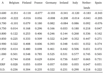
[Insert TABLE 2.4 about here]
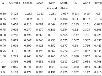
The results support a strong negative relationship between the level of disappointment aversion and the optimal weight of equities. This holds for all countries considered. More specifically, the results in Panel A suggest that investors should keep their equity exposure to a level higher than 50% (i.e., from 50.1% in Belgium to 78.5% in France) when preferences do not exhibit disappointment aversion (A = 1). However, as the level of DA increases (i.e.,A
declines), the optimal weight on equities becomes significantly lower and reaches negative values for very high levels of DA (i.e.,A ≤0.65). Also, the results show significantly different A∗ values across countries. For example, the presence of disappointment aversion depresses equity holdings more severely in Belgium (A∗ = 0.744) than in France (A∗= 0.629).
26 2.4 Empirical Results
significantly depressed as the level of DA increases. Third, when DA reaches very high levels, equity weights may even drop below zero, which means that an optimal investment strategy involves shorting (rather than holding) equities.
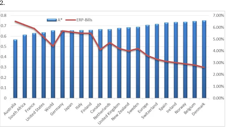
Figure 2.1 depicts A∗ values against equity premiums. It seems that higher equity premiums lead to smaller A∗ values for most countries. This implies that investors are less concerned about disappointment aversion when stocks significantly outperform T–bills. For example, France has a lower A∗ than Belgium (0.629 vs. 0.774), which is due to a much higher equity premium observed in the French equity market (5.7% vs. 2.8%). Moreover, it is also evident that A∗ values are driven not only by equity premiums but also by differences in stock market volatilities. Another example (see Finland vs. Italy) might help to explain this further. While both countries have an identical equity premium at 5.5%, the lower volatility of 29.0% in Italy (compared to 30.4% in Finland) leads into a lower A∗ (0.657 vs. 0.658). The mechanism that drives such a relationship is straightforward. Better market conditions (in the form of higher mean returns or lower volatilities) make risky investments (exposure to the equity market) more appealing. Investors therefore tend to be more resistant towards disappointment aversion. Additionally, higher expectations toward future profit opportunities may also attract new investors. Such effects help to further reduce the value ofA∗.
[Insert FIGURE 2.1 about here]
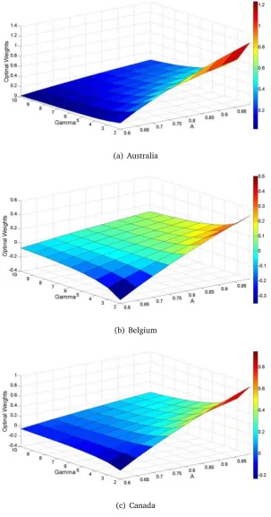
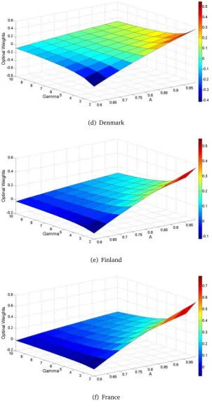
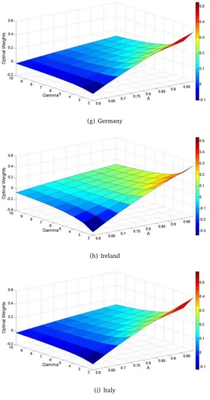
A = 1). For a given level of risk and disappointment aversion, equity exposure tends to increase either due to a higher equity premium or due to a lower standard deviation. Figure 2.2 also shows important differences in the shape of the 3D graphs across countries. This is mainly due to variations in risk and disappointment aversion, which both affect equity proportions in a non–linear way. More specifically, optimal equity holdings decline along with a higher risk aversion in a convex manner. This convexity is more pronounced at milder levels of disappointment aversion (i.e., when A values are greater than 0.85). In contrast, since the disappointment aversion parameter is multiplied by the disappointment–utility, an increasing disappointment aversion depresses equity holdings almost in a linear way. Furthermore, variations of disappointment aversion lead into a stronger impact on stock holdings when risk aversion is relatively low (i.e., for gamma values between 2 and 4). Overall, these findings strongly support the view that assessing investors’ risk attitudes with both risk and disappointment aversion grants a more reasonable solution to the equity premium puzzle around the world.
[Insert FIGURE 2.2 about here]
2.5 Conclusion
28 2.5 Conclusion
2.6 Tables & Figures of This Chapter
Table 2.1
Descriptive Statistics of Worldwide Equity Premiums
This table presents information about the level of equity premium for all countries considered in our analysis over the period 1900–2011. All data is obtained from the Global Investment Returns Yearbook 2012 and are also annualized.
Countries Equity Returns Bills Returns Equity premium Equity S.D.
Australia 7.20% 0.70% 6.50% 18.20%
Belgium 2.40% -0.40% 2.80% 23.60%
Canada 5.70% 1.60% 4.10% 17.20%
Denmark 4.90% 2.20% 2.70% 20.90%
Finland 5.00% -0.50% 5.50% 30.40%
France 2.90% -2.80% 5.70% 23.50%
Germany 2.90% -2.40% 5.30% 32.20%
Ireland 3.70% 0.70% 3.00% 23.10%
Italy 1.70% -3.60% 5.30% 29.00%
Japan 3.60% -1.90% 5.50% 29.80%
Netherlands 4.80% 0.70% 4.10% 21.80%
New Zealand 5.80% 1.70% 4.10% 19.70%
Norway 4.10% 1.20% 2.90% 27.30%
South Africa 7.20% 1.00% 6.20% 22.50%
Spain 3.40% 0.30% 3.10% 22.20%
Sweden 6.10% 1.80% 4.30% 22.90%
Switzerland 4.10% 0.80% 3.30% 19.70%
UK 5.20% 1.00% 4.20% 19.90%
US 6.20% 0.90% 5.30% 20.20%
Europe 4.60% 0.90% 3.70% 21.50%
30 2.6 Tables & Figures of This Chapter
Table 2.2
S&P 500 and Treasury Bill Returns from CRSP
This table presents descriptive statistics on equity returns (from S&P 500) and Treasury bill returns (90–day T–bills) over the period 1926–1998. This data is obtained from CRSP and used to replicate the optimal weights of Ang et al. (2005) for the case of the US market. All data are quarterly. Excess returns refer to stock returns in excess of T–bill returns. Its quarterly mean and standard deviation are calculated using the excess return series. Then the quarterly excess returns are annualised by multiplying four. Likewise, the standard deviations of quarterly excess returns are annualised by multiplying two.
Equity T–Bill Equity minus T–Bill
Mean Quarterly 2.66% 1.02% 1.64%
Annualized 10.64% 4.08% 6.56%
S.D. Quarterly 10.97% 0.86% 10.99%
Table 2.3
Replicating the Optimal Weights of Ang et al. (2005)
This table presents the optimal weights produced from our algorithm and compares them with those reported in Ang et al. (2005). For ease of comparison, we present results for different values of risk aversion (γ = 2 and γ = 5). The weight differences (Diff) is obtained using (our weights – Ang’s weights)/Ang’s weight.
Curvature Parameterγ = 2 Curvature Parameterγ = 5
A Ang’s weights Our weights Diff. Ang’s weights Our weights Diff.
1.00 0.927 0.932 0.539% 0.370 0.372 0.541%
0.95 0.833 0.839 0.720% 0.332 0.335 0.904%
0.90 0.734 0.741 0.954% 0.293 0.296 1.024%
0.85 0.628 0.638 1.592% 0.250 0.254 1.600%
0.80 0.517 0.528 2.128% 0.206 0.210 1.942%
0.75 0.398 0.411 3.266% 0.158 0.164 3.797%
0.70 0.271 0.286 5.535% 0.108 0.114 5.556%
32 2.6 Tables & Figures of This Chapter
Table 2.4
Optimal Portfolio Weights under Different A Values
This table reports the optimal portfolio weights for each of the 19 countries considered in our analysis. For ease of comparison with Ang et al. (2005), we set coefficient of risk aversion to 2 and report how the optimal weights change for different levels of disappointment aversion.
Panel A: Optimal Weights for Countries from the Eurozone
A Belgium Finland France Germany Ireland Italy Nether- Spain lands
0.600 -0.351 -0.118 -0.077 -0.103 -0.341 -0.120 -0.183 -0.343 0.650 -0.222 -0.016 0.056 -0.008 -0.208 -0.014 -0.041 -0.205 0.700 -0.101 0.079 0.180 0.082 -0.084 0.086 0.092 -0.076 0.750 0.014 0.168 0.296 0.166 0.033 0.180 0.218 0.047 0.800 0.122 0.253 0.406 0.246 0.144 0.268 0.336 0.162 0.850 0.225 0.333 0.509 0.322 0.249 0.352 0.447 0.271 0.900 0.322 0.408 0.606 0.393 0.348 0.431 0.552 0.374 0.950 0.414 0.480 0.698 0.461 0.442 0.506 0.651 0.472 1.000 0.501 0.548 0.785 0.525 0.531 0.577 0.745 0.565
Table 2.4 (continued)
Optimal Portfolio Weights under Different A Values
This table reports the optimal portfolio weights for each of the 19 countries considered in our analysis. For ease of comparison with Ang et al. (2005), we set coefficient of risk aversion to 2 and report how the optimal weights change for different levels of disappointment aversion.
Panel B: Optimal Weights for European Countries outside the Eurozone
A Denmark Norway Sweden Switzerland UK
0.60 -0.416 -0.291 -0.232 -0.35 -0.236
0.65 -0.269 -0.18 -0.097 -0.193 -0.08
0.70 -0.132 -0.076 0.029 -0.046 0.066
0.75 -0.002 0.023 0.148 0.092 0.203
0.80 0.12 0.117 0.26 0.222 0.333
0.85 0.236 0.205 0.366 0.345 0.454
0.90 0.345 0.289 0.466 0.461 0.569
0.95 0.449 0.369 0.561 0.571 0.678
1.00 0.548 0.444 0.651 0.676 0.781
A∗ 0.751 0.738 0.688 0.716 0.677
ERP 0.027 0.029 0.042 0.033 0.042
[image:43.595.126.513.209.477.2]34 2.6 Tables & Figures of This Chapter
Table 2.4 (continued)
Optimal Portfolio Weights under Different A Values
This table reports the optimal portfolio weights for each of the 19 countries considered in our analysis. For ease of comparison with Ang et al. (2005), we set coefficient of risk aversion to 2 and report how the optimal weights change for different levels of disappointment aversion.
Panel C: Optimal Weights for non–European Countries
A Australia Canada Japan New South US World Europe Zealand Africa
0.60 0.125 -0.233 -0.113 -0.261 -0.037 -0.114 -0.19 -0.3 0.65 0.297 -0.052 -0.01 -0.104 0.102 0.04 -0.014 -0.156 0.70 0.458 0.118 0.087 0.044 0.232 0.185 0.151 -0.022 0.75 0.608 0.277 0.179 0.183 0.354 0.32 0.305 0.105 0.80 0.748 0.426 0.265 0.313 0.468 0.447 0.45 0.224 0.85 0.879 0.567 0.346 0.436 0.575 0.567 0.587 0.337 0.90 1.003 0.699 0.423 0.552 0.677 0.68 0.716 0.443 0.95 1.12 0.825 0.496 0.662 0.772 0.787 0.837 0.544 1.00 1.229 0.943 0.566 0.766 0.863 0.888 0.952 0.64
[image:44.595.82.472.210.500.2]Figure 2.1
Equity Risk Premium vs. Disappointment Aversion
36 2.6 Tables & Figures of This Chapter
Figure 2.2
Optimal Weights under Different Risk and Disappointment Aversion This figure presents the optimal weights for each case considered (19 countries and two indices) across different levels of risk aversion (γ) and disappointment aversion (A).
(a) Australia
(b) Belgium
Figure 2.2 (continued)
Optimal Weights under Different Risk and Disappointment Aversion
(d) Denmark
(e) Finland
[image:47.595.148.451.154.737.2]38 2.6 Tables & Figures of This Chapter
Figure 2.2 (continued)
Optimal Weights under Different Risk and Disappointment Aversion
(g) Germany
(h) Ireland
[image:48.595.105.410.152.733.2]Figure 2.2 (continued)
Optimal Weights under Different Risk and Disappointment Aversion
(j) Japan
(k) Netherlands
[image:49.595.147.451.154.731.2]40 2.6 Tables & Figures of This Chapter
Figure 2.2 (continued)
Optimal Weights under Different Risk and Disappointment Aversion
(m) Norway
(n) South Africa
Figure 2.2 (continued)
Optimal Weights under Different Risk and Disappointment Aversion
(p) Sweden
(q) Switzerland
42 2.6 Tables & Figures of This Chapter
Figure 2.2 (continued)
Optimal Weights under Different Risk and Disappointment Aversion
(s) United States
(t) Europe
Chapter 3
A Cross–Cultural Study of Financial
Risk–Taking: Individualism and
Disappointment Aversion around
3.1 Introduction
Since the introduction of disappointment aversion (DA henceforth) of Gul (1991), the DA utility together with loss aversion has been widely used for the explanation of investors’ behaviour in financial markets. These utility functions, i.e., treating gains and losses rather than the total wealth and imposing heavier weights on disappointment (losses) than elation (gains), have attracted a lot of attention in the literature (e.g., Lien and Wang, 2002, 2003; Ang et al., 2005; Fielding and Stracca, 2007; Abdellaoui and Bleichrodt, 2007; Routledge and Zin, 2010; Gill and Prowse, 2012). However, the detailed specifications of these utility functions are not clear due to their unknown parameters, e.g., how investors’ respond to disappointment. Other characteristics of DA utility such as the relationship between DA and risk aversion or changes in DA to wealth levels have yet to be investigated. The purpose of this chapter is to scrutinise investors’ disappointment aversion and its impacts on asset pricing in order to answer these questions.
We propose a utility function that consists of wealth (consumption) utility as well as DA utility, as in Koszegi and Rabin (2007) and Barberis (2013). The wealth utility reflects the absolute utility from wealth levels which has been used in economics and finance, whereas the DA utility depends on gains and losses calculated with respect to the (endogenous) expected wealth. Our overall utility would help avoid misleading results by ignoring either gains and losses or wealth levels (Barberis, 2013). By interpreting the DA utility as a risk measure (Jia and Dyer, 1996) and assuming that utility is additively separable as in Koszegi and Rabin (2007). We analytically obtain several interesting relationships between the optimal investment proportions, levels of DA and risk aversion, expected excess returns, elation, and disappointment. The analytical relationships are then tested using asset allocations of pension funds in 35 OECD countries.
46 3.1 Introduction
more disappointment-averse. The former is well known: investors would not take additional risk unless properly compensated. The latter, however, seems counter-intuitive: investors who are more disappointment–averse would invest more in risky assets. But the counter–intuitive results are indeed consistent with the experimental findings of Abdellaoui and Bleichrodt (2007), because disappointment aversion increases when expected excess returns increase. That is, investors are particularly frustrated for suffering losses when they have a very good chance to win. Therefore, in bull markets when expected excess returns are high, both investment proportions in risky assets and disappointment aversion are high. With respect to wealth levels, if risk aversion decreases with wealth, i.e., decreasing absolute risk aversion holds, wealthier investors may feel more disappointment for losses.
These analytical results are supported by empirical results with asset allocation in pension funds of 35 OECD countries. The estimated DA levels (standard errors) of equities, bonds, and other investments (a portfolio of real estate, infrastructure, private equities and hedge funds) are 2.28 (0.31), 1.64 (0.17) and 1.93 (0.24), respectively. As predicted by the analytical results, DA is larger for equities whose expected returns are larger than those of the other risky assets. The large DA in equities could be a potential source of equity premium puzzle which is not well explained by risk.
The levels of DA are affected by wealth as well as individualism. As predicted by the analytical results, countries with larger wealth (measured by GDP) show higher levels of disappointment aversion for equities. Moreover, individualism of Hofstede (2001), a cultural character, appears to affect disappointment aversion. Individualistic countries appear to be more disappointment–averse than collectivistic countries. According to Van Den Steen (2004); Chui et al. (2010), individualistic investors tend to show more risk-taking activities in financial markets. Our results indicate that overconfidence of individualistic investors increases their expectations in risky assets, making themselves more disappointed for losses.
relationship with risk aversion and expected returns. The utility function we use for the asset allocation problem is a generalised one in the sense that it includes the aggregated wealth level as well as gains and losses. In contrast to other disappointment aversion utility functions defined solely over gains and losses, our utility also depend on the absolute pleasure of consumption purchased with wealth. Moreover, the assumption of additively separable utility allows us to apply the asset allocation problem for multiple risky assets11. In our framework, the overall utility is a linear combination of disappointment aversion utilities for multiple risky assets, and thus analysis becomes quite simple.
From the empirical side, our results show that cultural differences can play an important role in decision–making under risk, which is consistent with the view that investors from different backgrounds frame their risk attitude in different ways and are subject to psychological biases (e.g., Chui et al., 2010; Beugelsdijk and Frijns, 2010; Frijns et al., 2013; Breuer et al., 2014). In this study we show that disappointment aversion is also affected by cultural differences. The variation in disappointment aversion due to cultural difference challenges the traditional risk-based theories and contributes a new dimension to current behavioural literature.
The remainder of this chapter is organised as follows: in section 3.2 we propose our utility function and show how optimal asset allocation in risky assets are affected by risk and disappointment aversion. In section 3.3 we empirically test various analytical results developed in section 2. Section 3.4 focuses on discussions of the obtained results and concludes this chapter.
3.2 Disappointment Aversion in Asset Allocation
In this section, we propose a DA utility with subjective probability function and investigate how assets are allocated with respect to disappointment aversion. As in Koszegi and Rabin (2007), investors’ utility is assumed to depend on their multi– dimensional wealth portfolios (bundle) as well as reference portfolios under the
11Because of tractability, most previous studies focus on asset allocation problems with two assets,
48 3.2 Disappointment Aversion in Asset Allocation
assumption that utility is additively separable across different asset classes. We propose some analytical results between investment patterns, risk aversion, and disappointment aversion.
3.2.1 The Disappointment Aversion Utility
The DA utility is embedded in the asymmetric preference towards outcomes that do not meet a person’s prior expectation (disappointment) and those that exceed the expectation (elation): it predicts that the person reacts more sensitively to disappointment than to elation. Unlike loss aversion where the reference point is predetermined exogenously, the reference point in DA is endogenously decided depending on future return paths. Therefore, it is possible that the person still suffers disappointment even for a positive outcome if the outcome is lower than his expectations (reference points).
While the asymmetric preference with respect to disappointment and elation is a core of the DA utility, consumption levels are also what people care about. For example, Koszegi and Rabin (2007) propose a utility function in which consumption utility is considered in addition to the utility from gains and losses. As argued by Barberis (2013), neglecting consumption surely leads to biased conclusions. Therefore, our DA utility ((u(W, µs))consists of the typical wealth
utility and the disappointment–elation utility12. Formally, we have:
u(W, µs) =µw−ϕ
A|W −µw |v I−− |W −µw |v (1−I)−
, (3.1)
whereµw is the expected wealth, W represents the end–of–period wealth, andI−
is an indicator variable that equals one whenW−µw <0and zero otherwise. For
DA,A >1is required to give extra weights to the disappointment.
The first component of the DA utility is the expected end–of–period wealth
µw which represents utility from consumption via wealth. Similar to the models
of Koszegi and Rabin (2007), wealth utility (expected wealth) is differentiable and strictly increasing. Our DA utility increases linearly with expected wealth,
12For an application of DA utility in the asset allocation problem, we use the wealth level to
satisfying the non–satiation condition and allowing our model to be tractable (Barberis, 2013). The second component inside the square brackets in Eq. (3.1), which we refer to as the disappointment–elation utility, represents utility derived from gains and losses. The disappointment–elation utility, is also interpreted as a “standard measure of risk” (Jia and Dyer, 1996) or a performance measure (Gemmill et al., 2004). The parameter, ϕ > 0, thus, shows the relative importance of risk in the utility and represents thetrade–off relationship between wealth utility and risk: it is equivalent to a measure of risk aversion, which should decrease as wealth increases if decreasing absolute risk aversion holds. The curvature parameter, v, decides convexity or concavity of elation and disappointment with respect to gains and losses, respectively. As in many previous studies, the two curvature parameters for gains and losses are set equivalent to each other (e.g., see Tversky and Kahneman, 1992; Abdellaoui, 2000; Barberis et al., 2001; Ang et al., 2005; Abdellaoui and Bleichrodt, 2007). Finally, expected wealth is used as the reference point in this study. As pointed out by Koszegi and Rabin (2007), expected wealth is what people use to calculate gains and losses and is determined by rational expectations held in the recent past about outcomes.
3.2.2 Subjective Weighting Function
It is well–documented that people distort probabilities by disproportionately directing their attention to outcomes (Prelec, 1998). According to Tversky and Kahneman (1992), unlikely extreme outcomes are overweighted while highly possible events are underweighted. Quiggin (1995) introduces a rank–dependent utility model where weights depend on the true probability of an outcome as well as its ranking relative to other outcomes. The combination of rank and reference point–dependent utility gave birth to cumulative prospect theory (CPT), which utilizes a transformed probability weighting function to account for the redistribution of decision weights (Tversky and Kahneman, 1992).
50 3.2 Disappointment Aversion in Asset Allocation
parameter version of the weighting function:
w(p) =exp[−(ln(p))δ], (3.2) where p is the cumulative probability of any possible outcome. With δ (0 < δ < 1), the weighting function allocates more (fewer) weights to unlikely (likely) outcomes. A number of weighting functions (e.g., Prelec, 1998; Abdellaoui, 2000; Luce et al., 2000; Bruhin et al., 2010) have been proposed but they are quite similar to the weighting function of Prelec (1998), (see Gonzalez and Wu (1999) for example).
Although the rationale behind the subjective weighting is different from risk attitude toward gains and losses, they are closely connected. To see this, assume a transformed density function for elation and disappointment,π+(x)andπ−(x),
respectively, as follows:
π+(x) =w0(1−p)pdf(x),
π−(x) =w0(p)pdf(x),
where x = W −µw represents gains or losses, pdf(x) is the probability density
function of x; w0(1−p) and w0(p) are the first derivatives of Prelec’s (1998) weighting functions at the cumulative probabilities of1−pandp, respectively:
W0(1−p) = δ
1−p[(−ln(1−p))
δ−1exp(−(−ln(1−p))δ)], x≥0,
W0(p) = δ
p[(−lnp)
δ−1exp(−(−lnp)δ)], x <0,
Then the expected DA utility can be presented as:
UDA=E[u(W, µw)] =µw−ϕ[Apu−−(1−p)u+],
whereprepresents the cumulative probability at the reference point(x= 0), i.e.,
p=F(0), and
(1−p)u+ =
Z ∞
0
xvπ+(x)dx, pu−=
Z 0
−∞
The subjective weighting function is designed to replicate the probability distortion of outcomes, but alters the degree of risk attitude towards gains and losses for a given objective probability: for example,
xv[w0(p)pdf(x)] = [xvw0(p)]pdf(x). In other words, for a given objective probability, when combined with outcomes, the subjective weighting function creates concavity (risk aversion) for losses while it creates convexity (risk–loving) for gains. Even though the risk aversion for gains and risk–loving for losses are assumed for a given subjective weighting function, the net effects of the risk attitude and the subjective weighting function become unclear for a given objective probability.
Because of this lack of clarity between risk attitude and subjective weighting, it is difficult to estimate these two parameters simultaneously, i.e., the parameter of the weighting function and the curvature parameter. Moreover, as explained later, the DA parameter, A, is also closely associated with these two parameters. In order to minimize the difficulties in the estimation but keep the original rationale behind the DA utility and subjective weighting, we estimate DA for given subjective weighting and curvature. More specifically, we useδ = 0.74 for the subjective weighting as in Gonzalez and Wu (1999) and Hofstede’s (2001) “Uncertainty Avoidance” index for risk attitude, the details of which will be discussed later.
3.2.3 An Application to an Asset Allocation Problem
We consider an asset allocation problem for multiple asset classes, which is an extension of the typical asset allocation problem where only two types of assets (equity and risk–free asset) are considered (e.g., Ang et al., 2005; Fielding and Stracca, 2007; Hwang and Satchell, 2010). Suppose that the end–of–period wealth W is an outcome of a portfolio q where α1, α2, ..., αn of wealth are
invested in ntypes of risky asset, and the remaining(1−Pni=1αi) is invested in
the risk–free asset. Short positions are not allowed in a typical asset allocation in pension funds, suggesting 0 ≤ αi ≤ 1 for the i type of asset. Without loss of