Enhanced sharing analysis techniques: a comprehensive evaluation

(1)

evaluation

.

White Rose Research Online URL for this paper:

http://eprints.whiterose.ac.uk/1207/

Article:

Bagnara, R., Zeffanella, E. and Hill, P.M. (2005) Enhanced sharing analysis techniques: a

comprehensive evaluation. Theory and Practice of Logic Programming, 5 (1-2). pp. 1-43.

ISSN 1471-0684

https://doi.org/10.1017/S1471068404001978

[email protected] https://eprints.whiterose.ac.uk/ Reuse

See Attached

Takedown

If you consider content in White Rose Research Online to be in breach of UK law, please notify us by

(2)

DOI: 10.1017/S1471068404001978 Printed in the United Kingdom

Enhanced sharing analysis techniques:

a comprehensive evaluation

ROBERTO BAGNARA, ENEA ZAFFANELLA Department of Mathematics, University of Parma, Parma, Italy

(e-mail: {bagnara,zaffanella}@cs.unipr.it)

PATRICIA M. HILL†

School of Computing, University of Leeds, Leeds, UK (e-mail:[email protected])

Abstract

Sharing, an abstract domain developed by D. Jacobs and A. Langen for the analysis of logic programs, derives useful aliasing information. It is well-known that a commonly used core

of techniques, such as the integration ofSharingwith freeness and linearity information, can

significantly improve the precision of the analysis. However, a number of other proposals for refined domain combinations have been circulating for years. One feature that is common to these proposals is that they do not seem to have undergone a thorough experimental evaluation even with respect to the expected precision gains. In this paper we experimentally

evaluate: helping Sharingwith the definitely ground variables found usingPos, the domain

of positive Boolean formulas; the incorporation of explicit structural information; a full

implementation of the reduced product of Sharing and Pos; the issue of reordering the

bindings in the computation of the abstract mgu; an original proposal for the addition of a new mode recording the set of variables that are deemed to be ground or free; a refined way of using linearity to improve the analysis; the recovery of hidden information in the

combination ofSharingwith freeness information. Finally, we discuss the issue of whether

tracking compoundness allows the computation of more sharing information.

KEYWORDS: abstract interpretation, logic programming, sharing analysis, experimental evaluation

1 Introduction

In the execution of a logic program, two variables are aliased or share at some program point if they are bound to terms that have a common variable. Conversely, two variables are independent if they are bound to terms that have no variables in common. Thus by providing information about possible variable aliasing, we also

The work of the first and second authors has been partly supported by MURST projects “Certificazione automatica di programmi mediante interpretazione astratta” and “Interpretazione astratta, sistemi di tipo e analisi control-flow.”

(3)

provide information about definite variable independence. In logic programming, a knowledge of the possible aliasing (and hence definite independence) between variables has some important applications.

Information about variable aliasing is essential for the eﬃcient exploitation of AND-parallelism, Bueno et al. (1994, 1999); Chang et al. (1985) Hermenegildo and Greene (1990); Hermenegildo and Rossi (1995); Jacobs and Langen (1992); Muthukumar and Hermenegildo (1992). Informally, two atoms in a goal are executed in parallel if, by a mixture of compile-time and run-time checks, it can be guaranteed that they do not share any variable. This implies the absence ofbinding conflicts at run-time: it will never happen that the processes associated to the two atoms try to bind the same variable.

Another significant application isoccurs-check reduction, Crnogoracet al. (1996); Søndergaard (1986). It is well-known that many implemented logic programming languages (e.g. almost all Prolog systems) omit theoccurs-check from the unification procedure. Occurs-check reduction amounts to identifying the unifications where such an omission is safe, and, for this purpose, information on the possible aliasing of program variables is crucial.

Aliasing information can also be used indirectly in the computation of other interesting program properties. For instance, the precision with which freeness information can be computed depends, in a critical way, on the precision with which aliasing can be tracked, Bruynoogheet al. (1994a); Codishet al. (1993); Fil´e (1994); King and Soper (1994); Langen (1990); Muthukumar and Hermenegildo (1991).

In addition to these well-known applications, a recent line of research has shown that aliasing information can be exploited in Inductive Logic Programming (ILP). Several optimizations have been proposed for speeding up the refinement of induct-ively defined predicates in ILP systems, Blockeelet al. (2000); Santos Costa et al. (2000). It has been observed that the applicability of some of these optimizations, formulated in terms of syntactic conditions on the considered predicate, could be recast as tests on variable aliasing (Blockeelet al. 2000, Appendix D).

Sharing, a domain introduced in Jacobs, Langen Jacobs and Langen (1989, 1992); Langen (1990), is based on the concept of set-sharing. An element of the Sharing

domain, which is a set ofsharing-groups (i.e. a set of sets of variables), represents information on groundness,1 _{groundness dependencies, possible aliasing, and more} complexsharing-dependenciesamong the variables that are involved in the execution of a logic program, Bagnaraet al.(1997, 2002); Buenoet al. (1994, 1999).

Even though Sharing is quite precise, it is well-known that more precision is attainable by combining it with other domains. Nowadays, nobody would seriously consider performing sharing analysis without exploiting the combination of aliasing information with groundness and linearity information. As a consequence, expressions such as ‘sharing information’, ‘sharing domain’ and ‘sharing analysis’ usually capture groundness, aliasing, linearity and quite often also freeness. Notice

1 _{A variable is}_ground_{if it is bound to a term containing no variables, it is}_compound_{if it is bound to}

(4)

that this idiom is nothing more than a historical accident: as we will see in the sequel, compoundness and other kinds of structural information could also be included in the collective term ‘sharing information’.

As argued informally by Søndergaard (1986), linearity information can be suitably exploited to improve the accuracy of a sharing analysis. This observation has been formally applied in Codish et al. (1991) to the specification of the abstract mgu operator for ASub, a sharing domain based on the concept of pair-sharing (i.e. aliasing and linearity information is encoded by a set of pairs of variables). A similar integration with linearity for the domainSharing was proposed by Langen in his PhD thesis Langen (1990). The synergy attainable from the integration between aliasing and freeness information was pointed out by Muthukumar and Hermenegildo (1992). Building on these works, Hans and Winkler (1992) proposed a combined integration of freeness and linearity information with sharing, but small variations (such as the one we will present as the starting point for our work) have been developed by Bruynooghe and Codish (1993) and Bruynooghe et al.

(1994a).

There have been a number of other proposals for more refined combinations which have the potential for improving the precision of the sharing analysis over and above that obtainable using the classical combinations ofSharingwith linearity and freeness. These include the implementation of more powerful abstract semantic operators (since it is well-known that the commonly used ones are sub-optimal) and/or the integration with other domains. Not one of these proposals seem to have undergone a thorough experimental evaluation, even with respect to the expected precision gains. The goal of this paper is to systematically study these enhancements and provide a uniform theoretical presentation together with an extensive experimental evaluation that will give a strong indication of their impact on the accuracy of the sharing information.

Our investigation is primarily from the point of view of precision. Reasonable eﬃciency is also clearly of interest but this has to be secondary to the question as to whether precision is significantly improved: only if this is established, should better implementations be researched. One of the investigated enhancements is the integration of explicit structural information in the sharing analysis and an important contribution of this paper is that it shows both the feasibility and the positive impact of this combination.

Note that, regardless of its practicality, any feasible sharing analysis technique that oﬀers good precision may be valuable. While ineﬃciency may prevent its adoption in production analyzers, it can help in assessing the precision of the more competitive techniques.

(5)

Section 4 considers a simple combination of Pos with SFL; Section 5 investigates the eﬀect of including explicit structural information by means of the Pattern(·) construction; Section 6 discusses possible heuristic for reordering the bindings so as to maximize the precision ofSFL; Section 7 studies the implementation of a more precise combination betweenPosandSFL; Section 8 describes a new mode ‘ground or free’ to be included in SFL; Section 9 and Section 10 study the possibility of improving the exploitation of the linearity and freeness information already encoded in SFL. In Section 11 we discuss (without an experimental evaluation) whether compoundness information can be useful for precision gains. Section 12 concludes with some final remarks.

2 Preliminaries

For any setS,℘(S) denotes the powerset ofS. For ease of presentation, we assume there is a finite set of variables of interest denoted byVI. Iftis a syntactic object then

vars(t) andmvars(t) denote the set and the multiset of variables int, respectively. If aoccurs more than once in a multisetM we write aM. We letTerms denote the

set of first-order terms overVI.Bind denotes the set of equations of the formx=t where x∈ VI and t∈Terms is distinct from x. Note that we do not impose the occurs-check conditionx /∈vars(t), since we target the analysis of Prolog and CLP systems possibly omitting this check. The following simplification of the standard definitions for the Sharing domain given in Cortesi and Fil´e (1999); Hill et al. (1998); Jacobs and Langen (1992) assumes that the set of variables of interest is always given byVI.2

Definition 1

(Theset-sharing domain SH.)The setSH is defined by

SH def=℘(SG),

where the set ofsharing-groups SG is given by

SG def=℘(VI)\ {?}.

SH is ordered by subset inclusion. Thus the lub and glb of the domain are set union and intersection, respectively.

Definition 2

(Abstract operations over SH.)Theabstract existential quantification onSH causes an element of SH to “forget everything” about a subset of the variables of interest. It is encoded by the binary function aexists :SH×℘(VI)→SH such that,

2 _{Note that, during the analysis process, the set of variables of interest may expand (when solving the}

(6)

for eachsh ∈SH andV ∈℘(VI),

aexists(sh, V)def= {S\V |S∈sh, S \V =?} ∪ {{x} |x∈V}.

For eachsh ∈SH and eachV ∈℘(VI), the extraction of therelevant component of sh with respect to V is given by the function rel :℘(VI)×SH →SH defined as

rel(V ,sh)def={S ∈sh|S∩V =?}.

For each sh ∈SH and each V ∈℘(VI), the function rel : ℘(VI)×SH →SH

gives theirrelevant component of sh with respect toV. It is defined as

rel(V ,sh)def=sh\rel(V ,sh).

The function (·)⋆_:_SH _→_SH_{, also called} _star-union_{, is given, for each} _sh _∈_SH_,

by

sh⋆def=

S ∈SG

∃

n>₁.∃T1, . . . , Tn∈sh . S = n

i=1 Ti

.

For each sh1,sh2 ∈SH, the function bin :SH ×SH →SH, calledbinary union, is given by

bin(sh1,sh2) def

={S1∪S2|S1∈sh1, S2∈sh2}.

We also use theself-bin-union function sbin : SH →SH, which is given, for each

sh ∈SH, by

sbin(sh)def= bin(sh,sh).

The function amgu : SH ×Bind → SH captures the eﬀect of a binding on an element of SH. Assume (x = t) ∈ Bind, sh ∈ SH, Vx = {x}, Vt = vars(t), and

Vxt=Vx∪Vt. Then

amgu(sh, x=t)def= rel(Vxt,sh)∪bin(rel(Vx,sh)⋆,rel(Vt,sh)⋆). (1)

We now briefly recall the standard integration of set-sharing with freeness and linearity information. These properties are each represented by a set of variables, namely those variables that are bound to terms that definitely enjoy the given property. These sets are partially ordered byreverse subset inclusion so that the lub and glb operators are given by set intersection and union, respectively.

Definition 3

(The domain SFL.)Let Fdef=℘(VI) andLdef= ℘(VI) be partially ordered by reverse subset inclusion. The domain SFLis defined by the Cartesian product

SFLdef=SH ×F×L

ordered by the component-wise extension of the orderings defined on the three subdomains.

(7)

⊥ def= ?,VI,VI with all the elements corresponding to an impossible concrete computation state: for example, elements sh, f, l ∈ SFL such that f * vars(sh) (because a free variable does share with itself) orVI\vars(sh)*l(because variables that cannot share are also linear). Note however that these and other similar spurious elements rarely occur in practice and cannot compromise the correctness of the results.

In a bottom-up abstract interpretation framework, such as the one we focus on, abstract unification is the only critical operation. Besides unification, the analysis depends on the ‘merge-over-all-paths’ operator, corresponding to the lub of the domain, and the abstract projection operator, which can be defined in terms of an abstract existential quantification operator.

Definition 4

(Abstract operations over SFL.) The abstract existential quantification on SFL is encoded by the binary function aexists :SFL×℘(VI) →SFL such that, for each

d = sh, f, l ∈SFLandV ∈℘(VI),

aexists(d, V)def= aexists(sh, V), f∪V , l∪V.

For eachd = sh, f, l ∈SFL, we define the following predicates. The predicate

indd:Terms×Terms →Bool expresses definite independence of terms. Two terms s, t∈Terms areindependent in d if and only ifindd(s, t) holds, where

indd(s, t)

def

= (rel(vars(s),sh)∩rel(vars(t),sh) =?).

A termt∈Terms isfree in dif and only if the predicatefreed:Terms →Bool holds

fort, that is,

freed(t)def= (∃x∈VI . x=t∧x∈f).

A termt∈Terms is linear in d if and only iflind(t), wherelind:Terms →Bool is given by

lind(t)def= (vars(t)⊆l)

∧(∀x, y∈vars(t) :x=y∨indd(x, y))

∧(∀x∈vars(t) :xmvars(t)⇒_{x /}∈vars(sh)).

The function amgu :SFL×Bind →SFL captures the eﬀects of a binding on an element of SFL. Let (x =t) ∈ Bind and d = sh, f, l ∈ SFL. Let also Vx ={x},

Vt =vars(t),Vxt=Vx∪Vt,Rx= rel(Vx,sh) andRt= rel(Vt,sh). Then

(8)

where

sh′def= rel(Vxt,sh)∪bin(Sx, St);

Sx

def =

Rx, iffreed(x)∨freed(t)∨(lind(t)∧indd(x, t));

R⋆

x, otherwise;

St

def =

Rt, iffreed(x)∨freed(t)∨(lind(x)∧indd(x, t));

R⋆

t, otherwise;

f′def=           

f, iffreed(x)∧freed(t);

f\vars(Rx), iffreed(x);

f\vars(Rt), iffreed(t);

f\vars(Rx∪Rt), otherwise;

l′def= (VI \vars(sh′))∪f′∪l′′;

l′′def=           

l\(vars(Rx)∩vars(Rt)), iflind(x)∧lind(t);

l\vars(Rx), iflind(x);

l\vars(Rt), iflind(t);

l\vars(Rx∪Rt), otherwise.

This specification of the abstract unification operator is equivalent (modulo the lack of the explicit structural information provided byabstract equation systems) to that given in Bruynooghe et al. (1994a), providedx /∈vars(t). Indeed, as done in all the previous papers on the subject, in Bruynoogheet al. (1994a) it is assumed that the analyzed language does perform the occurs-check. As a consequence, whenever considering a definitely cyclic binding, that is a binding x=tsuch that x∈vars(t), the abstract operator can detect the definite failure of the concrete computation and thus return the bottom element of the domain. Such an improvement would not be safe in our case, since we also consider languages possibly omitting the occurs-check. However, when dealing with definitely cyclic bindings, the specification given by the previous definition can still be refined as follows.

Definition 5

(Improvement for definitely cyclic bindings.)Consider the specification of the abstract operations over SFL given in Definition 4. Then, whenever x ∈ vars(t), the computation of the new sharing component sh′ can be replaced by the following.3

sh′def= rel(Vxt,sh)∪bin(Sx,CSt),

where

CSt

def =

CRt, iffreed(x);

CR⋆t, otherwise;

CRt

def

= rel(vars(t)\ {x},sh).

3 _{Note that, in this special case, it also holds that}_free

(9)

This enhancement, already implemented in the China analyzer, is the rewording of a similar one proposed in Bagnara (1997) for the domain Pos in the context of groundness analysis. Its net eﬀect is to recover some groundness and sharing dependencies that are unnecessarily lost when using the standard operators.

The domainSH captures set-sharing. However, the property we wish to detect is

pair-sharingand, for this, it has been shown in Bagnaraet al. (2002) thatSH includes unwanted redundancy. The same paper introduces an upper-closure operatorρ on

SH and the domain PSD def= ρ(SH), which is the weakest abstraction of SH that isas precise as SH as far as tracking groundness and pair-sharing is concerned.4 _A notable advantage of PSD is that we can replace the star-union operation in the definition of the amgu by self-bin-union without loss of precision. In particular, in Bagnaraet al. (2002) it is shown that

amgu(sh, x=t) =ρrel(Vxt,sh)∪bin(sbin(rel(Vx,sh)),sbin(rel(Vt,sh))), (2)

where the notationsh1=ρsh2 meansρ(sh1) =ρ(sh2).

It is important to observe that the complexity of the amgu operator onSH (1) is exponential in the number of sharing-groups of sh. In contrast, the operator on PSD (2) is O(|sh|4_{). Moreover, checking whether a fixpoint has been reached} by testing sh1 =ρ sh2 has complexity O(|sh1|3+|sh2|3). Practically speaking, very often this makes the diﬀerence between thrashing and termination of the analysis in reasonable time.

The above observations onSHandPSDcan be generalized to apply to the domain combinations SFL and SFL2 def= PSD×F ×L. In particular, SFL2 achieves the same precision as SFL for groundness, pair-sharing, freeness and linearity and the complexity of the corresponding abstract unification operator is polynomial. For this reason, all the experimental work in this paper, with the exception of part of the one described in Section 7, has been conducted using theSFL2 domain.

3 Experimental evaluation

Since the main purpose of this paper is to provide an experimental measure of the precision gains that might be achieved by enhancing a standard sharing analysis with several new techniques we found in the literature, it is clear that the implementation of the various domain combinations was a major part of the work. However, so as to adapt these assorted proposals into a uniform framework and provide a fair comparison of their results, a large amount of underlying conceptual work was also required. For instance, almost all of the proposed enhancements were designed for systems that perform the occurs-check and some of them were developed for rather diﬀerent abstract domains: besides changing the representation of the domain elements, such a situation usually requires a reconsideration of the specification of the abstract operators.

4 _{The name}_PSD_{, which stands for}_{Pair-Sharing Dependencies}_{, was introduced in Zaﬀanella}_{et al}_{. (1999).}

(10)

All the experiments have been conducted using the China analyzer Bagnara (1997a) on a GNU/Linux PC system equipped with an AMD Athlon clocked at 700 MHz and 256 MB of RAM. China is a data-flow analyzer for CLP(HN)

languages (i.e. ISO Prolog, CLP(R),clp(FD) and so forth),HN being an extended

Herbrand system where the values of a numeric domain N can occur as leaves of the terms. China, which is written in C++, performs bottom-up analysis deriving

information on both call-patterns and success-patterns by means of program trans-formations and optimized fixpoint computation techniques. An abstract description is computed for the call- and success-patterns for each predicate defined in the program using a sophisticated chaotic iteration strategy proposed in Bourdoncle (1993a; 1993b).5

A major point of the experimental evaluation is given by the test-suite, which is probably the largest one ever reported in the literature on data-flow analysis of (constraint) logic programs. The suite comprises all the programs we have access to (i.e. everything we could find by systematically dredging the Internet): more than 330 programs, 24 MB of code, 800 K lines. Besides classical benchmarks, several real programs of respectable size are included, the largest one containing 10063 clauses in 45658 lines of code. The suite also comprises a few synthetic benchmarks, which are artificial programs explicitly constructed to stress the capabilities of the analyzer and of its abstract domains with respect to precision and/or eﬃciency.

Because of the exponential complexity of the base domain SFL, a data-flow analysis that includes this domain will only be practical if it incorporates widening operators such as those proposed in Zaffanellaet al. (1999).6 _{However, since almost} none of the investigated combinations come with specialized widening operators, for a fair assessment of the precision improvements we decided to disable all the widenings available in our SFL implementation. As a consequence, there are a few benchmarks for which the analysis does not terminate in reasonable time or absorbs memory beyond acceptable limits, so that a precision comparison is not possible. Note however that the motivations behind this choice go beyond the simple observation that widening operators affect the precision of the analysis: the problem is also that, if we use the widenings defined and tuned for our implementation of the domain SFL, the results would be biased. In fact, the definition of a good widening for an analysis domain normally depends on both the representation and the implementation of the domain. In other words, different implementations even of the same domain will require different tunings of the widening operators (or even, possibly, brand new widenings). This means that adopting the same widening operators for all the domain combinations would weaken, if not invalidate, any conclusions regarding the relative benefits of the investigated enhancements. On the other hand, the definition of a new specialized widening operator for each one of the considered domain combinations, besides being a formidable task, would also be

5 _China _{uses the recursive fixpoint iteration strategy on the weak topological ordering defined by}

partitioning of the call graph into strongly-connected subcomponents, Bourdoncle (1993b).

6 _{Note that we use the term ‘widening operator’ in its broadest sense: any mechanism whereby, in the}

(11)

wasted eﬀort as the number of benchmark programs for which termination cannot be obtained within reasonable time is really small.

For space reasons, the experimental results are only summarized here. The interested reader can find more information (including a description of the constantly growing benchmark suite and detailed results for each benchmark) at the URI

http://www.cs.unipr.it/China/. Indeed, given the high number of benchmark

programs and the many domain combinations considered,7 _{even finding a concise,} meaningful and practical way to summarize the results has been a non-trivial task.

For each benchmark, precision is measured by counting the number of independ-ent pairs (the corresponding columns are labeled ‘I’ in the tables) as well as the numbers of definitely ground (labeled ‘G’), free (‘F’) and linear (‘L’) variables detected by each abstract domain. The results obtained for diﬀerent analyses are compared by computing the relative precision improvements or degradations on each of these quantities and expressing them using percentages. The “overall” (‘O’) precision improvement for the benchmark is also computed as the maximum improvement on all the measured quantities.8 _{The benchmark suite is then partitioned into several} precision equivalence classes: the cardinalities of these classes are expressed again using percentages. For example, when looking at the precision results reported in Table 1 for goal-dependent analysis, the value 2.3 that can be found at the intersection of the row labeled ‘0< p 6_{2’ with the column labeled ‘G’ is to be} read as follows: “for 2.3 percent of the benchmarks the increase in the number of ground variables is less than or equal to 2 percent.” The precision class labeled ‘unknown’ identifies those benchmarks for which a precision comparison was not possible, because one or both of the analyses was timed-out (for all comparisons, the time-out threshold is 600 seconds). In summary, a precision table gives an approximation of the distribution of the programs in the benchmark suite with respect to the obtained precision gains.

For a rough estimate of the efficiency of the different analyses, for each comparison we provide two tables that summarize the times taken by the fixpoint computations. It should be stressed that these by no means provide a faithful account of the intrinsic computational cost of the tested domain combinations. Besides the lack of widenings, which have a big impact on performance as can be observed by the results reported in Zaffanella et al. (1999), the reader should not forget that, for ease of implementation, having targeted at precision we traded efficiency whenever possible. Therefore, these tables provide, so to speak, upper-bounds: refined implementations can be expected to perform at least as well as those reported in the tables.

As done for the precision results, the timings are summarized by partitioning the suite into equivalence classes and reporting the cardinality of each class using

7 _{We compute the results of 40 diﬀerent variations of the static analysis, which are then used to perform}

36 comparisons. The results are computed over 332 programs for goal-independent analyses and over 221 programs for goal-dependent analyses. This diﬀerence in the number of benchmarks considered comes from the fact that many programs either are not provided with a set of entry goals or use constructs such ascall(G)whereGis a term whose principal functor is not known. In these cases the analyzer recognizes that goal-dependent analysis is pointless, since no call-patterns can be excluded.

8 _{When computing this “overall” result for a benchmark, the presence of even a single precision loss}

(12)

percentages. In the first table we consider the distribution of the absolute time diﬀerences, that is we measure the slow-down and speed-up due to the incorporation of the considered enhancement. Note that the class called ‘same time’ actually comprises the benchmarks having a time diﬀerence below a given threshold, which is fixed at 0.1 seconds. In the second table we show the distribution of the total fixpoint computation times, both for the base analysis (in the columns labeled ‘%1’) and for the enhanced one (in the columns labeled ‘%2’); the columns labeled ‘∆’ show how much each total time class grows or shrinks due to the inclusion of the considered combination.

4 A simple combination with Pos

It is well-known that the domain Sharing (and thus also SFL) keeps track of ground dependencies. More precisely,SharingcontainsDef, the domain of definite Boolean functions defined in Armstronget al. (1998), as a proper subdomain defined in Cortesi et al. (1992); Zaﬀanella et al. (1999). However, we consider here the combination ofSFL withPos, the domain of positive Boolean functions defined in Armstronget al. (1998). There are several good reasons to coupleSFLwithPos:

1. Pos is strictly more expressive than Def in that it can represent (positive) disjunctive groundness dependencies that arise in the analysis of Prolog pro-grams, Armstronget al. (1998). The ability to deal with disjunctive dependencies is also needed for the precise approximation of the constraints of some CLP languages: for example, when using the finite domain solver of SICStus Prolog, the user can write disjunctive constraints such as ‘X #= 4 #\/ Y #= 6’. 2. The increased precision on groundness propagates to the SFL component. It

can be exploited to remove redundant sharing groups and to identify more linear variables, therefore having a positive impact on the computation of the amgu operator of the SFL domain. Moreover, when dealing with sequences of bindings, the added groundness information allows them to be usefully reordered. In fact, while it has been proved in Hill et al.(1998) that Sharing

alone is commutative, meaning that the result of the analysis does not depend on the ordering in which the bindings are executed the domainSFL does not enjoy this property. In particular, even for the simpler combination ofSharing

with linearity it has been known since Langen (1990, pp. 66–67) that better results are obtained if thegrounding bindingsare considered before the others.9 As an example, consider the sequences of unifications (f(X, X, Y) =A, X=a) and (X =a, f(X, X, Y) =A) (Langen 1990, p. 66). The combination withPos

is clearly advantageous in this respect.

3. Besides being useful for improving precision on other properties, disjunctive dependencies also have a few direct applications, such as occurs-check reduc-tion. As observed in Crnogorac et al. (1996), if the groundness formulax∨y

9 _{A binding}_x₌_t_is_grounding_{with respect to an abstract description if, in all the concrete computation}

states approximated by the abstract description, either the variablexis ground or all the variables in

(13)

holds, the unificationx=yis occurs-check free, even when neitherxnory are definitely linear.

4. Detecting the set of definitely ground variables through Posand exploiting it to simplify the operations on SFL can improve the eﬃciency of the analysis. In particular this is true if the set of ground variables is readily available, as is the case, for instance, with the GER implementation ofPosin Bagnara and Schachte (1999).

5. The combination withPosis essential for the application of a powerful widening technique onSFLas described in Zaﬀanellaet al. (1999). This is very important, since analysis based onSFL is not practical without widenings.

6. In the context of the analysis of CLP programs, the notions of “ground variable” and the notion of “variable that cannot share a common variable with other variables” are distinct. A numeric variable in, say, CLP(R), cannot share with other numerical variables (not in the sense of interest in this paper) but is not ground unless it has been constrained to a unique value. Thus the analysis of CLP programs with SFL alone either will lose precision on pair-sharing (if arithmetic constraints are abstracted into “sharings” among numeric variables in order to approximate the groundness of the latter) or will be imprecise on the groundness of numeric variables (because only Herbrand constraints take part in the construction of sharing-sets). In the first alternative, as we have already noted, the precision with which groundness of numeric variables can be tracked will also be limited. Since groundness of numeric variables is important for a number of applications (e.g. compiling equality constraints down to assignments or tests in some circumstances), we advocate the use ofPosandSFL at the same time.

Thus, as a first technique to enhance the precision of sharing analysis, we consider the simple propagation of the set of definitely ground variables from the Pos

component to theSFLcomponent.10 _{We denote this domain by}_Pos_×_SFL_. As noted above, the GER implementation of Bagnara and Schachte (1999), besides being the fastest implementation ofPosknown to date, is the natural candidate for this combination, since it provides constant-time access to the setGof the definitely ground variables. Note that the widenings on thePoscomponent have been retained. The reason for this choice is that they fire for only a few benchmarks and, when coming into play, they rarely aﬀect the precision of the groundness analysis: by switching them oﬀ we would only obtain a few more time-outs.

In theSFLcomponent, the setGof definitely ground variables is used

• to reorder the sequence of bindings in the abstract unification so as to handle the grounding ones first;

• to eliminate the sharing groups containing at least one ground variable; and • to recover from previous linearity losses.

The experimental results forPos×SFLare compared with those obtained for the domainSFLconsidered in isolation and reported in Table 1. It can be observed that

(14)

[image:14.493.83.398.64.481.2]

Table 1. SFL2 versus Pos×SFL2

Goal independent Goal dependent

Prec. class O I G F L O I G F L

5< p610 – – – – – 0.5 – 0.5 – –

2< p65 0.3 – 0.3 – – – – – – –

0< p62 0.6 0.6 0.6 – 0.6 3.2 3.6 2.3 – 2.7

Same precision 95.8 96.1 95.8 96.7 96.1 92.8 92.8 93.7 96.4 93.7

Unknown 3.3 3.3 3.3 3.3 3.3 3.6 3.6 3.6 3.6 3.6

% benchmarks

Time diﬀerence class Goal Ind. Goal Dep.

degradation>1 2.7 6.8

0.5<degradation61 1.5 0.5

0.2<degradation60.5 3.0 0.9

both timed out 3.3 3.6

same time 81.6 81.9

0.1<improvement60.2 – 0.5

0.2<improvement60.5 0.9 0.5

0.5<improvement61 0.3 –

improvement>1 0.9 0.5

Goal Ind. Goal Dep.

Total time class %1 %2 ∆ %1 %2 ∆

timed out 3.3 3.3 – 3.6 3.6 –

t >10 8.4 9.0 0.6 7.2 7.2 – 5< t610 0.6 0.3 −0.3 1.4 1.4 – 1< t65 6.6 7.5 0.9 3.2 3.6 0.5 0.5< t61 3.3 2.7 −0.6 5.4 5.4 – 0.2< t60.5 7.2 8.4 1.2 10.4 13.1 2.7

t60.2 70.5 68.7 −1.8 68.8 65.6 −3.2

a precision improvement is observed in all of the measured quantities but freeness, aﬀecting up to 3.6% of the programs.

Note that there is a small discrepancy between these results and those of Bagnara

et al. (2000) where more improvements were reported. The reason is that the current

SFLimplementation uses an enhanced abstract unification operator, fully exploiting the anticipation of the grounding bindings even on the base domain SFL itself. In contrast, in the earlier SFL implementation used for the results in Bagnara et al. (2000), only thesyntactically grounding bindings were anticipated.11

11 _{A binding} _x₌ _t_{is syntactically grounding if}_vars₍_t_{) =}_?_{. This “syntactic” definition diﬀers from}

(15)

As for the timings, even if the figures in the tables seem to contradict what we claimed in point 4 above, a closer inspection of the detailed results reveals that this is only due to a very unfortunate interaction between the increased precision given byPosand the absence of widening operators on SFL. This state of aﬀairs forces the analyzer to compute a few, but very expensive, further iterations in the fixpoint computation.

Because of the reasons detailed above, we believePosshould be part of the global domain employed by any “production analyzer” for CLP languages. That is why, for the remaining comparisons, unless otherwise stated, this simple combination with thePosdomain is always included.

5 Tracking explicit structural information

A way of increasing the precision of almost any analysis domain is by enhancing it with structural information. For mode analysis, this idea dates back to Janssens and Bruynooghe (1992). A more general technique was proposed in Cortesiet al. (1994), where the generic structural domain Pat(ℜ) was introduced. A similar proposal, tailored to sharing analysis, is due to Bruynooghe et al. (1994a), where abstract equation systems are considered. In the experimental evaluation the Pattern(·) construction (Bagnara 1997a; 1997b; Bagnaraet al. 2000) is used. This is similar to

Pat(ℜ) and correctly supports the analysis of languages omitting the occurs-check in the unification procedure as well as those that do not.

The construction Pattern(·) upgrades a domainD (which must support a certain set of basic operations) with structural information. The resulting domain, where structural information is retained to some extent, is usually much more precise than D alone. There are many occasions where these precision gains give rise to consistent speed-ups. The reason for this is twofold. First, structural information has the potential of pruning some computation paths on the grounds that they cannot be followed by the program being analyzed. Second, maintaining a tuple of terms with many variables, each with its own description, can be cheaper than computing a description for the whole tuple Bagnara et al. (2000). Of course, there is also a price to be paid: in the analysis based on Pattern(D), the elements of Dthat are to be manipulated are often bigger (i.e. there are more variables of interest) than those that arise in analyses that are simply based onD.

When comparing the precision results, the diﬀerence in the number of variables tracked by the two analyses poses a non-trivial problem. How can we provide a

(16)

Consider a simple but not trivial Prolog program: mastermind.12 _{Consider also} the only direct query for which it has been written, ‘?- play.’, and focus the attention on the procedure extend code/1. A standard goal-dependent analysis of the program with the Pos×SFL domain cannot say anything on the successes of

extend code/1. If the analysis is performed with Pattern(Pos×SFL) the situation

changes radically. Here is what such a domain allows Chinato derive:13

extend_code([([A|B],C,D)|E]) :-list(B), list(E),

(functor(C,_,1);integer(C)), (functor(D,_,1);integer(D)),

ground([C,D]), may_share([[A,B,E]]).

This means: “during any execution of the program, whenever extend code/1

succeeds it will have its argument bound to a term of the form[([A|B],C,D)|E], whereBandEare bound to list cells (i.e. to terms whose principal functor is either

’.’/2 or []/0); C and D are ground and bound to a functor of arity 1 or to

an integer; and pair-sharing may only occur among A, B, and E”. Once structural information has been discarded, the analysis with Pattern(Pos×SFL) only specifies

thatextend code/1may succeed. Thus, according to our approach to the precision

comparison, explicit structural information gives no improvements in the analysis of

extend code/1(which is far from being a fair conclusion).

Of course, structural information is very valuable in itself. For example, when exploited for optimized compilation it allows for enhanced clause indexing and sim-plified unification. Several other semantics-based program manipulation techniques (such as debugging, program specialization, and verification) benefit from this kind of information. However, the value of this extra precision could only be measured from the point of view of the target application of the analysis.

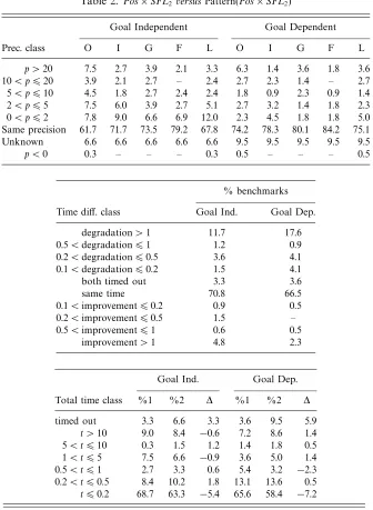
Thus the precision of the domainPos×SFLhas been compared with that obtained using the domain Pattern(Pos×SFL) and the results reported in Table 2. It can be seen that, for goal-independent analysis, on one third of the benchmarks compared there is a precision improvement in at least one of the measured quantities; the same happens for one sixth of the benchmarks in the case of goal-dependent analysis. Moreover, the increase in precision can be considerable, as testified by the percentages of benchmarks falling in the higher precision classes.

The reader may be surprised, as the authors were, to see that in some cases the precision actually decreased.14 _{Indeed, to the best of our knowledge, this possibility} has escaped all previous research work investigating this kind of abstract domain enhancement, including Cortesiet al. (1994), Bruynoogheet al. (1994a) and Bagnara

12 _{This program which implements the game “Mastermind” was rewritten by H. Koenig and T. Hoppe}

after code by M. H. van Emden and available at http://www.cs.unipr.it/China/Benchmarks/ Prolog/mastermind.pl.

13 _{Some extra groundness information obtained by the analysis has been omitted for simplicity: this says}

that, ifAandBturn out to be ground, thenEwill also be ground.

14 _{This happens for the program}_attractions2_{in the case of goal-independent analysis and for the}

(17)

[image:17.493.87.423.58.517.2]

Table 2. Pos×SFL2 versusPattern(Pos×SFL2)

Goal Independent Goal Dependent

p >20 7.5 2.7 3.9 2.1 3.3 6.3 1.4 3.6 1.8 3.6 10< p620 3.9 2.1 2.7 – 2.4 2.7 2.3 1.4 – 2.7 5< p610 4.5 1.8 2.7 2.4 2.4 1.8 0.9 2.3 0.9 1.4 2< p65 7.5 6.0 3.9 2.7 5.1 2.7 3.2 1.4 1.8 2.3 0< p62 7.8 9.0 6.6 6.9 12.0 2.3 4.5 1.8 1.8 5.0

Same precision 61.7 71.7 73.5 79.2 67.8 74.2 78.3 80.1 84.2 75.1

Unknown 6.6 6.6 6.6 6.6 6.6 9.5 9.5 9.5 9.5 9.5

p <0 0.3 – – – 0.3 0.5 – – – 0.5

% benchmarks

Time diﬀ. class Goal Ind. Goal Dep.

same time 70.8 66.5

0.1<improvement60.2 0.9 0.5

0.2<improvement60.5 1.5 –

0.5<improvement61 0.6 0.5

improvement>1 4.8 2.3

Goal Ind. Goal Dep.

timed out 3.3 6.6 3.3 3.6 9.5 5.9

t >10 9.0 8.4 −0.6 7.2 8.6 1.4 5< t610 0.3 1.5 1.2 1.4 1.8 0.5 1< t65 7.5 6.6 −0.9 3.6 5.0 1.4 0.5< t61 2.7 3.3 0.6 5.4 3.2 −2.3 0.2< t60.5 8.4 10.2 1.8 13.1 13.6 0.5 t60.2 68.7 63.3 −5.4 65.6 58.4 −7.2

(1997a). The reason for these precision losses lies in a subtle interaction between the explicit structural information and the underlying abstract unification operator.

(18)

principal functor f/2, the abstract computation should proceed by evaluating, on the base domainPos×SFL, the set of bindings{y=g(w), z=w}. Here the problem is that, as already noted, the amgu operator on the base domainPos×SFL is not commutative. While this improvement in the data used by the abstract computation very often allows for a corresponding increase in the precision of the result, in rare situations it may happen that a sub-optimal ordering of the bindings is chosen, incurring a precision loss.

It should be noted that such a negative interaction with the explicit struc-tural information is only possible when the underlying domain implements non-commutative abstract operators. In particular, this phenomenon could not be observed when computing on Pattern(SH) or Pattern(Pos).

One issue that should be resolved is whether the improvements provided by explicit structural information subsume those previously obtained for the simple combination withPos. Intuitively, it would seem that this cannot happen, since these two enhancements are based on different kinds of information: while the Pattern(·) construction encodes somedefinite structural information, the precision gain due to usingPosrather than justDef only stems fromdisjunctivegroundness dependencies. However, the impact of these techniques on the overall analysis is really intricate and some overlapping cannot be excluded a priori: for instance, both techniques affect the ordering of bindings in the computation of abstract unification onSFL. In order to provide some experimental evidence for this qualitative reasoning, the precision results are computed for the simpler domain Pattern(SFL) and then compared with those obtained for the domain Pattern(Pos×SFL). Since the main differences between Tables 1 and 3 can be explained by discrepancies in the numbers of programs that timed-out, these results confirm our expectations that these two enhancements are effectively orthogonal.

Similar experimental evaluations, but based on the abstract equation systems of Bruynooghe et al. (1994a), were reported by Mulkers et al. (1994, 1995). Here a depth-k abstraction (replacing all subterms occurring at a depth greater than or equal to k with fresh abstract variables) is conducted on a small benchmark suite (19 programs) for values ofk between 0 and 3. The domain they employed was not suitable for the analysis of real programs and, in fact, even the analysis of a modest-sized program like ann could only be carried out with depth-0 abstraction (i.e. without any structural information). Such a problem in finding practical analyzers that incorporated structural information with sharing analysis was not unique to this work: there was at least one other previous attempt to evaluate the impact of structural information on sharing analysis that failed because of combinatorial explosion (A. Cortesi, personal communication, 1996).

(19)

[image:19.493.95.416.62.487.2]

Table 3. Pattern(SFL2)versusPattern(Pos×SFL2)

5< p610 – – – – – 0.5 – 0.5 – –

2< p65 0.3 – 0.3 – – – 0.5 – – –

0< p62 – – – – – 3.2 3.2 2.7 – 2.7

Same precision 93.1 93.4 93.1 93.4 93.4 86.4 86.4 86.9 90.0 87.3

Unknown 6.6 6.6 6.6 6.6 6.6 10.0 10.0 10.0 10.0 10.0

% benchmarks

Time diﬀ. class Goal Ind. Goal Dep.

same time 75.6 73.8

0.1<improvement60.2 – –

0.2<improvement60.5 0.6 –

0.5<improvement61 – –

improvement>1 – 0.5

Goal Ind. Goal Dep.

timed out 6.6 6.6 – 10.0 9.5 −0.5

t >10 8.1 8.4 0.3 7.7 8.6 0.9 5< t610 1.5 1.5 – 2.3 1.8 −0.5 1< t65 5.1 6.6 1.5 4.5 5.0 0.5 0.5< t61 3.9 3.3 −0.6 3.2 3.2 – 0.2< t60.5 7.2 10.2 3.0 10.9 13.6 2.7

t60.2 67.5 63.3 −4.2 61.5 58.4 −3.2

The results obtained in this section demonstrate that there is a relevant amount of sharing information that is not detected when using the classical set-sharing domains. Therefore, in order to provide an experimental evaluation that is as systematic as possible, in all of the remaining experiments the comparison is performed both with and without explicit structural information.

6 Reordering the non-grounding bindings

(20)

the grounding bindings are considered first. This heuristic, which has been used for all the experiments in this paper, is well-known: in the literature all the examples that illustrate the non-commutativity of the abstract mgu onSFL use a grounding binding. However, as observed in Section 5, the problem is more general than that.

To illustrate this, suppose thatVI ={u, v, w, x, y, z}is the set of relevant variables, and consider theSFLelement15

d def= {vy, wy, xy, yz},?,{u, x, z},

where no variable is free and u, x, and z are linear with the bindings v = w and x=y. Then, applying amgu to these bindings in the given ordering, we have:

d1= amgu(d, v=w)

= {vwy, xy, yz},?,{u, x, z},

d1,2= amgu(d1, x=y)

= {vwxy, vwxyz, xy, xyz},?,{u, z}.

Using the reverse ordering, we have:

d2= amgu(d, x=y)

= {vwxy, vwxyz, vxy, vxyz, wxy, wxyz, xy, xyz},?,{u, z},

d2,1= amgu(d2, v=w)

= {vwxy, vwxyz, xy, xyz},?,{u}.

Thus d2,1 loses the linearity ofz (which, in turn, could cause bigger precision losses later in the analysis).

In principle, optimality can be obtained by adopting the brute-force approach: trying all the possible orderings of the non-grounding bindings. However, this is clearly not feasible. While lacking a better alternative, it is reasonable to look for heuristic that can be applied in the context of alocal search paradigm: at each step, the next binding for the amgu procedure is chosen by evaluating the eﬀect of its abstract execution, considered in isolation, on the precision of the analysis.

Suppose the number of independent pairs is taken as a measure of precision. Then, at each step, for each of the bindings under consideration, the new component

sh′, as given by Definition 4, must be computed. However, because the computation of sh′ is the most costly operation to be performed in the computation of the amgu operator, a direct application of this heuristic does not appear to be feasible. As an alternative, consider a heuristic based on the number of star-unions that have to be computed. Star-unions are likely to cause large losses in the number of independent pairs that are found. As only non-grounding bindings are considered, any binding requiring the computation of a star-union will need the star-union even if it is delayed, although a binding that does not require the star-union may require it if its computation is postponed: its variables may lose their freeness,

(21)

linearity or independence as a result of evaluating the other bindings. It follows that one potential heuristic is: “delay the bindings requiring star-unions as much as possible”. In the next example, by adopting this heuristic, the linearity of variabley is preserved.

Consider the application of the bindingsx=zandv=wto the following abstract description:

d def= {vw, wx, wy, z},?,{u, v, x, y}.

Since x is linear and independent from z, computing amgu(d, x = z) requires one star-union, while two star-unions are needed when computing amgu(d, v=w) because v and w may share. Thus, with the proposed heuristic, x =z is applied beforev=w, giving:

d1= amgu(d, x=z)

= {vw, wxz, wy},?,{u, v, y},

d1,2= amgu(d1, v=w)

= {vw, vwxyz, vwxz, vwy},?,{u, y}.

In contrast, ifv=w is applied first, we have:

d2= amgu(d, v=w)

= {vw, vwx, vwxy, vwy, z},?,{u, x, y},

d2,1= amgu(d2, x=z)

= {vw, vwxyz, vwxz, vwy},?,{u}.

Note that the same number of independent pairs is computed in both cases. It should be noted that this heuristic, considered in isolation, is not a general solution and can actually lead to precision losses. The problem is that, if a binding that needs a star-union is delayed, then, when the star-union is computed, it may be done on a larger sharing-set, forcing more (independent) pairs of variables into the same sharing group.

Consider the application of the bindings u = x and v = w to the abstract description

d def= {u, uw, v, w, xy, xz},{u, x},{u, x}.

Sincexanduare both free variables, no star-union is needed in the computation of amgu(d, u=x), while two star-unions are needed when computing amgu(d, v=w).

d1= amgu(d, u=x)

= {uwxy, uwxz, uxy, uxz, v, w},{u, x},{u, x},

d1,2= amgu(d1, v=w)

(22)

Using the other ordering, we have:

d2= amgu(d, v=w)

= {u, uvw, vw, xy, xz},{x},{x},

d2,1= amgu(d2, u=x)

= {uvwxy, uvwxz, uxy, uxz, vw},?,?.

Note that in d2,1 variablesy andzare independent, whereas they may share ind1,2. Thus, in this example, by delaying the only binding that requires the star-unions, v=w, the number of known independent pairs is decreased.

Another possibility is to consider a heuristic that uses the numbers of free and linear variables as a measure of precision for local optimization. That is, it chooses first those bindings for which these numbers are maximal. However, the last example shown above is evidence that even such a proposal may also cause precision losses (the binding u=xwould be chosen first as it preserves the freeness of variableu).

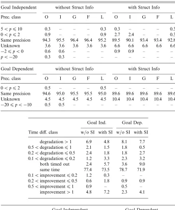
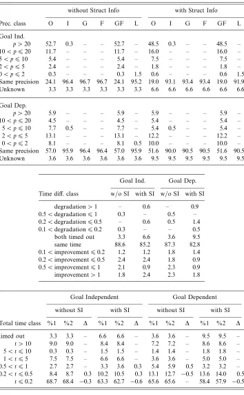
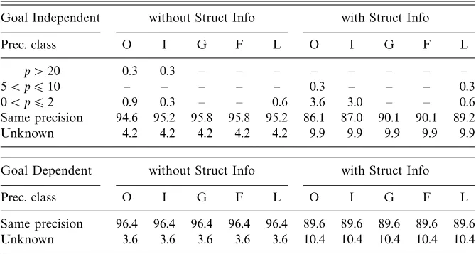
To evaluate the eﬀects of these two heuristic on real programs, we have implemen-ted and compared them with respect to the “straight” abstract computation, which considers the non-grounding bindings using the left-to-right order.16 _{The results} reported in Tables 4 and 5 can be summarized as follows:

1. the precision on the groundness and freeness components is not aﬀected; 2. the precision on the independent pairs and linearity components is rarely

aﬀected, in particular when considering goal-dependent analyses;

3. even for real programs, as was the case for the artificial examples given above, the precision can be increased as well as decreased.

Looking at Tables 4 and 5, it can be seen that the heuristic based on freeness and linearity information is slightly better than the use of the straight order, which, in its turn, is slightly better than the heuristic based on the number of star-unions.

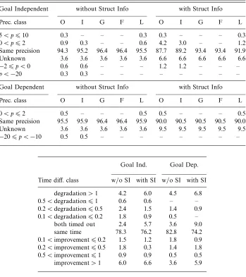
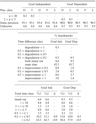
Clearly, since these results could not be generalized to other orderings, our investigation cannot be considered really conclusive. Besides designing “smarter” heuristic, it would be interesting to provide a kind of responsiveness test for the underlying domain with respect to the choice of ordering for the non-grounding bindings: a simple test consists in measuring how much the precision can be aﬀected, in either way, by the application of an almost arbitrary order. This is the motivation for the comparison reported in Table 6, where the order is from right-to-left, the reverse of the usual one. As for the results given in Tables 4 and 5, the number of changes to the precision observed in Table 6 is small and all the observations made above still hold. Surprisingly, this reversed ordering provides marginally better precision results than those obtained using the considered heuristic.17

16 _{The base domain is}_Pos_×_SFL_{, both with and without structural information.}

17 _{It is worth noting that the only precision improvement reported in Table 6 for the goal-dependent}

(23)

Table 4. The heuristic based on the number of star-unions

Goal Independent without Struct Info with Struct Info

0< p62 0.9 – – – 0.9 – – – – –

Same precision 94.6 95.5 96.4 96.4 95.5 91.3 91.3 93.1 93.1 93.1

Unknown 3.6 3.6 3.6 3.6 3.6 6.9 6.9 6.9 6.9 6.9

−26p <0 0.9 0.9 – – – 1.8 1.8 – – –

Goal Dependent without Struct Info with Struct Info

Same precision 96.4 96.4 96.4 96.4 96.4 90.5 90.5 90.5 90.5 90.5

Unknown 3.6 3.6 3.6 3.6 3.6 9.5 9.5 9.5 9.5 9.5

Goal Ind. Goal Dep.

Time diﬀ. class w/o SI with SI w/o SI with SI

degradation>1 4.5 3.0 7.2 4.1

0.5<degradation61 0.6 0.3 – –

0.2<degradation60.5 2.4 0.9 0.5 0.5

0.1<degradation60.2 1.5 0.6 0.5 0.5

both timed out 3.0 6.3 3.6 9.5

same time 80.7 80.7 85.5 76.9

0.1<improvement60.2 1.5 1.2 0.5 0.5

0.2<improvement60.5 1.8 1.2 1.4 2.3

0.5<improvement61 0.9 0.6 – 0.9

improvement>1 3.0 5.1 0.9 5.0

without SI with SI without SI with SI

Total time class %1 %2 ∆ %1 %2 ∆ %1 %2 ∆ %1 %2 ∆

timed out 3.3 3.3 – 6.6 6.6 – 3.6 3.6 – 9.5 9.5 –

t >10 9.0 8.1 −0.9 8.4 9.0 0.6 7.2 7.7 0.5 8.6 8.1 −0.5 5< t610 0.3 0.9 0.6 1.5 1.2 −0.3 1.4 0.9 −0.5 1.8 2.7 0.9 1< t65 7.5 7.5 – 6.6 6.3 −0.3 3.6 3.2 −0.5 5.0 4.1 −0.9 0.5< t61 2.7 2.4 −0.3 3.3 3.0 −0.3 5.4 5.9 0.5 3.2 3.6 0.5 0.2< t60.5 8.4 9.3 0.9 10.2 10.5 0.3 13.1 12.7 −0.5 13.6 13.1 −0.5

t60.2 68.7 68.4 −0.3 63.3 63.3 – 65.6 66.1 0.5 58.4 58.8 0.5

7 The reduced product between Pos and Sharing

(24)

[image:24.493.66.409.68.480.2]

Table 5. The heuristic based on freeness and linearity

5< p610 0.3 – – – 0.3 0.3 – – – 0.3

0< p62 0.9 – – – 0.9 2.7 2.4 – – 0.3

Same precision 94.3 95.5 96.4 96.4 95.2 89.5 90.1 93.4 93.4 92.8

Unknown 3.6 3.6 3.6 3.6 3.6 6.6 6.6 6.6 6.6 6.6

−26p <0 0.6 0.6 – – – 0.9 0.9 – – –

p <−20 0.3 0.3 – – – – – – – –

0< p62 0.5 – – – 0.5 – – – – –

Same precision 94.6 95.0 95.5 95.5 95.0 89.6 89.6 89.6 89.6 89.6

Unknown 4.5 4.5 4.5 4.5 4.5 10.4 10.4 10.4 10.4 10.4

−206p <−10 0.5 0.5 – – – – – – – –

Goal Ind. Goal Dep.

degradation>1 6.9 4.8 8.1 7.7

0.5<degradation61 2.1 1.5 1.8 0.5

0.2<degradation60.5 2.4 1.8 1.8 2.7

0.1<degradation60.2 1.2 3.3 2.3 3.2

same time 77.4 73.5 78.7 71.9

0.1<improvement60.2 1.2 0.3 – –

0.2<improvement60.5 0.6 1.8 0.9 0.9

0.5<improvement61 0.9 – 0.5 –

improvement>1 4.8 7.2 2.3 4.1

Total time class %1 %2 ∆ %1 %2 ∆ %1 %2 ∆ %1 %2 ∆

timed out 3.3 2.7 −0.6 6.6 5.7 −0.9 3.6 4.5 0.9 9.5 10.0 0.5

t >10 9.0 9.6 0.6 8.4 8.7 0.3 7.2 6.8 −0.5 8.6 7.7 −0.9 5< t610 0.3 2.1 1.8 1.5 1.8 0.3 1.4 1.4 – 1.8 2.7 0.9 1< t65 7.5 6.0 −1.5 6.6 6.9 0.3 3.6 4.5 0.9 5.0 5.0 – 0.5< t61 2.7 3.0 0.3 3.3 3.9 0.6 5.4 4.1 −1.4 3.2 3.6 0.5 0.2< t60.5 8.4 9.9 1.5 10.2 13.3 3.0 13.1 13.1 – 13.6 15.4 1.8

(25)

[image:25.493.81.430.70.463.2]

Table 6. Reversing the ordering of the non-grounding bindings

5< p610 0.3 – – – 0.3 0.3 – – – 0.3

0< p62 0.9 0.3 – – 0.6 4.2 3.0 – – 1.2

Same precision 94.3 95.2 96.4 96.4 95.5 87.7 89.2 93.4 93.4 91.9

Unknown 3.6 3.6 3.6 3.6 3.6 6.6 6.6 6.6 6.6 6.6

−26p <0 0.6 0.6 – – – 1.2 1.2 – – –

p <−20 0.3 0.3 – – – – – – – –

0< p62 0.5 – – – 0.5 0.5 – – – 0.5

Same precision 95.5 95.9 96.4 96.4 95.9 90.0 90.5 90.5 90.5 90.0

Unknown 3.6 3.6 3.6 3.6 3.6 9.5 9.5 9.5 9.5 9.5

−206p <−10 0.5 0.5 – – – – – – – –

Goal Ind. Goal Dep.

degradation>1 4.2 6.0 4.5 6.8

0.5<degradation61 0.6 0.6 – –

0.2<degradation60.5 2.4 1.5 1.4 0.9

0.1<degradation60.2 1.8 0.9 0.5 –

same time 78.3 76.2 82.8 74.2

0.1<improvement60.2 1.5 1.2 1.8 0.9

0.2<improvement60.5 1.8 0.3 1.4 1.8

0.5<improvement61 0.9 0.9 0.5 0.5

improvement>1 6.0 6.6 3.6 5.9

Total time class %1 %2 ∆ %1 %2 ∆ %1 %2 ∆ %1 %2 ∆

timed out 3.3 2.7 −0.6 6.6 5.7 −0.9 3.6 3.6 – 9.5 9.0 −0.5

t >10 9.0 8.7 −0.3 8.4 9.9 1.5 7.2 7.7 0.5 8.6 8.1 −0.5 5< t610 0.3 1.8 1.5 1.5 1.5 – 1.4 0.5 −0.9 1.8 2.7 0.9 1< t65 7.5 6.9 −0.6 6.6 6.0 −0.6 3.6 3.2 −0.5 5.0 4.5 −0.5 0.5< t61 2.7 2.4 −0.3 3.3 2.7 −0.6 5.4 5.4 – 3.2 3.6 0.5 0.2< t60.5 8.4 8.7 0.3 10.2 11.1 0.9 13.1 13.1 – 13.6 12.2 −1.4

(26)

contains redundancy, that is, there is more than one element that can characterize the same set of concrete computational states.

In Bagnara et al. (2000), two techniques that are able to remove some of this redundancy were experimentally evaluated. One of these aims at identifying those pairs of variables (x, y) for which the Boolean formula of the Pos component implies the binary disjunction x∨y. In such a case, it is always safe to assume that the variables x andy are independent.18 _{Since the number of independent pairs is} one of the quantities explicitly measured, this enhancement has the potential for “immediate” precision gains. The other technique exploits the knowledge of the sets of ground-equivalent variables: the variables in e ⊆ VI are ground-equivalent in φ ∈Pos if and only if, for each x, y ∈ e, φ|= (x ↔y). For a description of how these sets can be used to improve sharing analysis, the reader is referred to Bagnara

et al. (2000). The main motivation for experimenting with this specific reduction was the ease of its implementation, since all the needed information can easily be recovered from the already computedEcomponent of the GER implementation of

Pos in Bagnara and Schachte (1999). The experimental evaluation results given in Bagnara et al. (2000) for these two techniques show precision improvements with only three of the programs and, also, only with respect to the number of independent pairs that were found. Those results just apply to these limited forms of reduction, so could not be considered a complete account of all the possible precision gains.

The full reduced product defined in Cousot and Cousot (1979) betweenPosand

Sharing has been elegantly characterized in Codishet al. (1999), where set-sharing

`

a la Jacobs and Langen is expressed in terms of elements of thePosdomain itself. Let [φ]VI denote the set of all the models of the Boolean functionφdefined over the

set of variablesVI. Then, the isomorphism maps each set-sharing elementsh∈SH

into the Boolean formulaφ∈Possuch that

[φ]VI ={VI\S|S∈sh} ∪ {VI}.

The sharing information encoded by an element (φg, φsh) ∈ Pos×Pos can be

improved by replacing the second component (that is, the Boolean formula describing set-sharing information) with the conjunction φg∧φsh. The reader is referred to

Codish et al. (1999) for a complete account of this composition and a justification of its correctness.

This specification of the reduced product can be reformulated, using the standard set-sharing representation for the second component, to define a reduction procedure reduce :Pos×SH →SH such that, for allφg∈Pos,sh∈SH,

reduce(φg,sh) ={S∈sh |(VI \S)∈[φg]VI}.

The enhanced integration ofPosandSFL, based on the above reduction operator, is denoted here by Pos⊗SFL. From a formal point of view, this isnot the reduced product between Pos and SFL: while there is a complete reduction between Pos

andSH, the same does not necessarily hold for the combination with freeness and linearity information. Also note that the domain Pos⊗SFLis strictly more precise

(27)

[image:27.493.82.423.67.299.2]

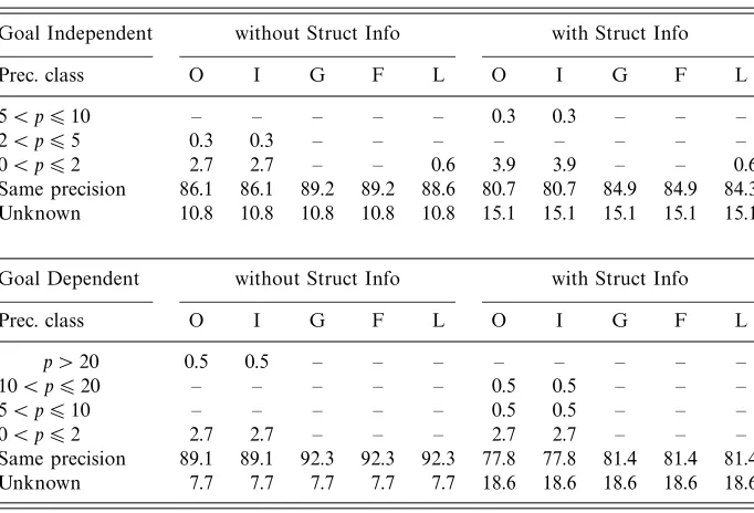
Table 7. Pos×SFL2 versus Pos⊗SFL

5< p610 – – – – – 0.3 0.3 – – –

2< p65 0.3 0.3 – – – – – – – –

0< p62 2.7 2.7 – – 0.6 3.9 3.9 – – 0.6

Same precision 86.1 86.1 89.2 89.2 88.6 80.7 80.7 84.9 84.9 84.3

Unknown 10.8 10.8 10.8 10.8 10.8 15.1 15.1 15.1 15.1 15.1

p >20 0.5 0.5 – – – – – – – –

10< p620 – – – – – 0.5 0.5 – – –

5< p610 – – – – – 0.5 0.5 – – –

0< p62 2.7 2.7 – – – 2.7 2.7 – – –

Same precision 89.1 89.1 92.3 92.3 92.3 77.8 77.8 81.4 81.4 81.4

Unknown 7.7 7.7 7.7 7.7 7.7 18.6 18.6 18.6 18.6 18.6

than the domainShPSh_{, defined in Scozzari (2000) for pair-sharing analysis. This is}

because the domainShPSh is the reduced product of a strict abstraction ofPosand a strict abstraction ofSH.

When using the domain PSD in place of SH, the ‘reduce’ operator specified above can interact in subtle ways with an implementation removing theρ-redundant sharing groups from the elements ofPSD. The following is an example where such an interaction provides results that are not correct.

Let VI = {x, y, z} and sh = {xy, xz, yz, xyz} ∈ PSD be the current set-sharing description. Suppose that the implementation internally representssh by using the ρ-reduced elementshred ={xy, xz, yz}, so thatsh =ρ(shred). Suppose also that the groundness description computed on the domainPos is φg = (x ↔y ↔z). Note

that we have [φg]VI ={?,{x, y, z}}. Then we have

sh′= reduce(sh, φg) ={xyz};

sh′red = reduce(shred, φg) =?.

The twoPos-reduced elementssh′andsh′red are not equivalent, even moduloρ. Note that the above example does not mean that the reduced product between

Posand PSD yields results that are not correct; neither does it mean that it is less precise than the reduced product betweenPosandSH for the computation of the observables. More simply, the optimizations used in our current implementation of

(28)

The precision comparison provides empirical evidence that Pos⊗SFL is more eﬀective than the combination considered in Bagnara et al. (2000). However, as indicated by the number of time-outs reported in Table 7, using Pos⊗SFL is not feasible due to its intrinsic exponential complexity. We deliberately decided not to include the time comparison, since it would have provided no information at all: the eﬃciency degradations, which are largely caused by the lack ofρ-reductions, should not be attributed to the enhanced combination withPos. In this respect, the reader looking for more details is referred to Bagnaraet al. (2000).

For the only purpose of investigating how many precision improvements may have been missed in the previous comparison due to the high number of time-outs, we have performed another experimental evaluation where we have compared the base domain Pos×SFL2 and the domain Pos⊗SFL2. We stress the fact that, given the observation made previously, such a precision comparison provides an

over-estimation for the actual improvements that can be obtained by a correct integration of the ρ-reduction and the ‘reduce’ operators. A detailed investigation of the experimental data, which cannot be reported here for space reasons, has shown that the number of precision improvements shown in Table 7 could at most double. In particular, improvements are more likely to occur for goal-independent analyses.

8 Ground-or-free variables

Most of the ideas investigated in the present work are based on earlier work by other authors. In this section, we describe one originally proposed in Bagnaraet al. (2000). Consider the analysis of the binding x = t and suppose that, on a set of computation paths, this binding is reached with x ground while, on the remaining computation paths, the binding is reached withxfree. In both casesxwill be linear and this is all that will be recorded when using the usual combination Pos×SFL. This information is valuable since, in the case that x and t are independent, it allows the star-union operation for the relevant component for t to be dispensed with. However, the information that is lost, that is, x being either ground or free, is equally valuable, since this would allow the avoidance of the star-union of both

the relevant components for x and t, even when x andt may share. This loss has the disadvantages that CPU time is wasted by performing unnecessary but costly operations and that the precision is potentially degraded: not only are the extra star-unions useless for correctness but may introduce redundant sharing groups to the detriment of accuracy. It is therefore useful to track the additional mode ‘ground-or-free’.

The analysis domainSFLis extended with the componentGFdef=℘(VI) consisting of the set of variables that are known to be either ground or free. As for freeness and linearity, the approximation ordering onGFis given by reverse subset inclusion. When computing the abstract mgu on the new domain

(29)

the property of being ground-or-free is used and propagated in almost the same way as freeness information.

Definition 6

(Improved abstract operations over SGFL.)Let d = sh, f,gf, l ∈SGFL. We define the predicate gfreed:Terms →Bool such that, for each first order term t, where

Vt

def

= vars(t)⊆VI,

gfreed(t)

def

= (rel(Vt,sh) =?)∨(∃x∈VI . x=t∧x∈gf).

Consider the specification of the abstract operations overSFLgiven in Definition 4. The improved operator amgu :SGFL×Bind→SGFLis given by

amgu(d, x=t)def= sh′, f′,gf′, l′,

wheref′andl′′are defined as in Definition 4 and

sh′= rel(Vxt,sh)∪bin(Sx, St);

Sx=

Rx, ifgfreed(x)∨gfreed(t)∨(lind(t)∧indd(x, t));

R⋆x, otherwise;

St =

Rt, ifgfreed(x)∨gfreed(t)∨(lind(x)∧indd(x, t));

R⋆

t, otherwise;

gf′= (VI\vars(sh′))∪gf′′;

gf′′=      

    

gf, ifgfreed(x)∧gfreed(t); gf \vars(Rx), ifgfreed(x);

gf \vars(Rt), ifgfreed(t); gf \vars(Rx∪Rt), otherwise;

l′=gf′∪l′′.

The computation of the set gf′′ is very similar to the computation of the set f′ as given in Definition 4. The new ground-or-free component gf′ is obtained by adding to gf′′ the set of all the ground variables: in other words, if a variable “loses freeness” then it also loses its ground-or-free status unless it is known to be definitely ground. It can be noted that, in the computation of this improved amgu, the ground-or-free property takes the role previously played by freeness. In particular, when computing sh′, all the tests for freeness have been replaced by tests on the newly defined Boolean function gfreed; similarly, in the computation

of the new linearity component l′, the set f′ has been replaced by gf′ (since any ground-or-free variable is also linear). It is also easy to generalize the improvement for definitely cyclic bindings introduced in Definition 5 to the domain SGFL: as before, the testfreed(x) needs to be replaced with the new testgfreed(x).