The identification of complex spatiotemporal patterns using Coupled map lattice model

This is a repository copy of The identification of complex spatiotemporal patterns using

Coupled map lattice model.

White Rose Research Online URL for this paper:

http://eprints.whiterose.ac.uk/74569/

Monograph:

Pan, Y. and Billings, S.A. (2006) The identification of complex spatiotemporal patterns

using Coupled map lattice model. Research Report. ACSE Research Report no. 923 .

Automatic Control and Systems Engineering, University of Sheffield

[email protected] Reuse

Unless indicated otherwise, fulltext items are protected by copyright with all rights reserved. The copyright exception in section 29 of the Copyright, Designs and Patents Act 1988 allows the making of a single copy solely for the purpose of non-commercial research or private study within the limits of fair dealing. The publisher or other rights-holder may allow further reproduction and re-use of this version - refer to the White Rose Research Online record for this item. Where records identify the publisher as the copyright holder, users can verify any specific terms of use on the publisher’s website.

Takedown

If you consider content in White Rose Research Online to be in breach of UK law, please notify us by

The Identification of Complex Spatiotemporal Patterns Using

Coupled Map Lattice model

Pan, Y. and Billings, S. A.

Department of Automatic Control and Systems Engineering

University of Sheffield

Sheffield, S1 3JD

UK

The Identification of Complex Spatiotemporal

Patterns Using Coupled Map Lattice Models

Pan, Y. and Billings, S. A.

Department of Automatic Control & Systems Engineering

Sheffield University,

Sheffield, S1 3JD, UK

May, 2006

Abstract

Many complex and interesting spatiotemporal patterns have been ob-served in a wide range of scientific areas. In this paper, two kinds of spatiotemporal patterns including spot replication and Turing systems are investigated and new identification methods are proposed to obtain Coupled Map Lattice (CML) models for this class of systems. Initially, a new correlation analysis method is introduced to determine an appropriate temporal and spatial data sampling step procedure for the identification of spatiotemporal systems. A new combined Orthogonal Forward Regres-sion and Bayesian Learning algorithm with Laplace priors is introduced to identify sparse and robust CML models for complex spatiotemporal patterns. The final identified CML models are validated using correlation based model validation tests for spatiotemporal systems. Numerical re-sults illustrate the identification procedure and demonstrate the validity of the identified models.

1

Introduction

Spatiotemporal systems can give rise to many complex and interesting phe-nomena such as self-organized, oscillatory and chaotic patterns. Initially, spa-tiotemporal phenomena were observed and studied in chemical reactions which can display periodic or chaotic temporal oscillations and pattern formation. By the early 1920s, Lotka had developed a simple model in terms of partial dif-ferential equations, based on two sequential autocatalytic reactions, which can produce sustained oscillations.

model and can show a variety of interesting spatial and temporal phenomena. Over the past decade, some scientists discovered that by changing one or two critical parameters nonlinear chemical dynamics can also exhibit fascinating self-organized patterns such as spiral waves, spatial chaos, crystal lattices and Turing structures [24] [32] [46] [48].

Recently, a lot of attention had been focused on the study of spatiotemporal models of interacting populations in nature [3] [25]. Maron and Harrison [35] investigated extensively a host-parasitoid system relating to the dynamics of the western tussock moth and its natural enemies. The low mobility of tussock moths, their high parasitism rates and the high mobility of the parasitoids altogether can form a self-organized pattern as predicted by Turing theory [37]. Turing patterns are a kind of spatiotemporal system that can produce steady state heterogeneous spatial patterns under certain initial and boundary condi-tions. This type of phenomena, termed diffusion-driven instability, was first investigated by Turing in 1952 in the field of chemistry. In his seminal pa-per, Turing demonstrated theoretically that a system of reacting and diffusing chemicals could spontaneously evolve to spatially heterogeneous patterns from an initially uniform state in response to infinitesimal perturbations. Turing pat-terns were first observed in chemical experiments as late as 1990 [7] [10] [40] by using the Lengyel-Epstein model [29]. Turing systems have also been shown to be able to at least qualitatively imitate many biological patterns such as the stripes of a zebra or spots of a cheetah and even more irregular patterns such as those on leopards and giraffes. Also the skin of exotic fish, butterflies or beetles can be imitated by using the Turing model [2] [41].

Another interesting spatiotemporal behavior of spot self-replication was first observed by Pearson [44] during his intensive investigation of the numerical simulation of the diffusive Gray-Scott system. This pattern is composed of a population of chemical spots that divide into daughter spots upon growth and decay with over-population. The pattern formation of self-replicating spots was experimentally confirmed by Lee et al. [27] [28] in chemical systems. It can also be seen that the dynamics of spots are similar to living cells that are undergoing mitosis. The dynamics of spot self-replicatiion has been theoretically studied in the one, two and three dimensional cases [36]. In addition, Nishiura and Ueyama [38] proposed a theoretical mechanism that drives the replication dynamics from a global bifurcation point of view. The study of the dynamics of spot self-replication was extended in the noise-controlled Gray-Scott model [30].

lattice where each site evolves in time through a discrete map which describes the influence of the past state and neighboring sites. A CML can be used to model dynamical behaviors that are normally described by partial differential equations. But the computational efficiency is greatly enhanced when using CML models compared with PDEs. It has been shown that CML models can exhibit complex spatiotemporal behaviors, including chaos, intermittency, trav-eling waves and Turing patterns [23]. Consequently, CML models have been used to study spatiotemporal systems in a wide class of scientific subjects.

The identification and forecasting of CML models from observed spatiotem-poral data has recently been studied using various methods [8] [9] [15] [19] [34] [33] [43] [39]. There are two main methods in studying the identification and forecasting problem for spatiotemporal systems. One approach uses embed-ding to reconstruct the local model describing the underlying dynamics. The other approach uses the orthogonal least square algorithms to identify the CML model. However, most of these methods have only been applied to relatively simple classes of spatiotemporal systems. In this paper, a new and effective approach for the identification of CML models for complex spatiotemporal pat-terns is proposed. The new identification method is composed of two parts. First, a new correlation analysis method is introduced to select appropriate sampling intervals of the identification data in the time and space domains. This method is based on the nonlinear auto-correlation functions of the output variables of spatiotemporal systems. The identification of CML models from noisy observed data is achieved using a new Orthogonal Forward Regression algorithm with Bayesian learning theory to provide a sparse model to fit the complex spatiotemporal dynamics with good generalization error.

The paper is arranged as follows. Section 2 gives a general description of the CML model and the identification procedure for spatiotemporal systems using regression methods. Section 3 introduces the new correlation based method to determine accurate sampling values of spatiotemporal data for identification. A new identification method using the OFR algorithm and Bayesian Learning theory with Laplace priors is then proposed to obtain CML models for com-plex spatiotemporal patterns. Section 4 introduces the correlation based model validation tests for spatiotemporal systems to validate the final identified CML models. Finally, numerical examples using spot-replicating patterns and Turing patterns are included in section 5 to illustrate the application of the new identi-fication methods and to demonstrate the accuracy and effectiveness of identified models for complex spatiotemporal patterns.

2

Problem Formulation

Consider the general form of the stochastic input-output CML model for time and spatially invariant lattice dynamical systems[8] [9]

where i ∈ Id _{is the spatial index of a d-dimensional space and t ∈ T is the} temporal index;yi(t) and ui(t) are the output and input variables respectively at latticeiand timet, andεi(t) is an independent zero mean random sequence.

qn_{(t) is a temporal backward shift operator}

qn = (q−1_{, q}−2_{, ..., q}−n_{) (2)}

so that

qny_y

i(t) = (yi(t−1), yi(t−2), ..., yi(t−ny))

qnu_u

i(t) = (ui(t−1), ui(t−2), ..., ui(t−nu))

qnε_ε

i(t) = (εi(t−1), εi(t−2), ..., εi(t−nε))

(3)

whereny, nu, nε denote the maximum temporal lags corresponding to output

y, inputuand the residual sequence ε.

In (1),sm_{is a multi valued spatial shift operator}

sm_{= (s}p1_{, s}p2_{, ..., s}pm_{) (4)} wherepj _∈Id _{is the spatial translation multi index, such that}

smy_y

i = (yi−p1, y_i−p2, ..., y_i−pmy)

smu_u

i= (ui−p1, u_i−p2, ..., u_i−pmu)

smε_ε

i= (εi−p1, ε_i−p2, ..., ε_i−pmε)

(5)

The parametersmy,muandmεdenote the maximum spatial radius correspond-ing to the outputy, input uand the residual sequence ε. The task of system identification for spatiotemporal systems is to obtain the unknown CML model

f(·) from observed data.

In practice, the underlying spatiotemporal system for identification evolves continuously in time over a specific spatial domain. Therefore, it is essential to choose an appropriate sampling timeTtand space gridTsbefore the spatiotem-poral data for identification is collected. There seem to be virtually no results in the literature relating to this important problem. In many situations, the form of the CML modelf(·) is unknown, so it is necessary to expandf using a known set of possible candidate model terms. Equation(1) can also be written in the regression format which is constructed as a linear combination of a finite number of model terms.

yi(t) =

X

k

θi,kϕi,k(t) +εi(t) (6)

Therefore, the identification task for spatiotemporal systems involves the following steps.

(a) Choose an appropriate sampling timeTs and spatial grid Ss according to the inherent characteristics of the spatiotemporal data.

(b) Determine the regressor set. This step involves choosing the nonlinear de-gree, values of maximum temporal lags for inputs and outputsnu and ny and maximum spatial radiusmuand my.

(c) Select the proper model terms that can adequately represents the underlying spatiotemporal system.

(d) Estimate the parameters associated with the model terms.

Each step in the identification procedure will be discussed in detail in the fol-lowing sections.

3

The Identification of CML models for

Com-plex Pattern Formation

In this section, a practical approach for selecting appropriate sampling intervals of spatiotemporal data in both the space and time domains is investigated. An Orthogonal Forward Regression algorithm and Bayesian learning theory with Laplace priors is then introduced to select appropriate model terms and to give unbiased estimates of the model parameters.

3.1

The Selection of Sampling intervals in the space-time

domain

It is well known that the sampling interval of continuously observed purely tem-poral data for identification can influence the selection of the model structure and parameter estimation during nonlinear temporal system identification [4]. The maximum lagsnu andny also vary as the sampling timeTschanges. Fur-thermore, if the data are over-sampled, the design matrix can become ill-posed due to the high correlation between successive measurements. On the other hand, if the data for identification are under-sampled, important information will be lost. In this situation, the final derived model is likely to be sensitive to new training data or the noise and consequently cannot generalize well.

should not be uncorrelated, the sampling time should be long enough so as to avoid over-correlation. Actually, the selection of the sampling time is often a compromise between the over-correlation and the uncorrelated situations. In this paper, the correlation method based on the linear and nonlinear correlation functions applied in the nonlinear temporal system identification is extended to determine the sampling intervals of data in both the time and space domains of spatiotemporal data.

The correlation functions for spatiotemporal systems are composed of two parts with respect to the sampling intervals in the time and space domain re-spectively. In this method,Nssamples of the original spatiotemporal data from outputs are randomly selected over both the space and time domain. The cor-relation functions for the sampling time of spatiotemporal data are defined as follows

Φ(yyt)(τt) =

PS(Ns−1)

(i,t)=S(0)(yi(t)−y)(yi(t−τt)−y)

PS(Ns−1)

(i,t)=S(0)(yi(t)−y)2 Φ(_yt2)_y2(τt) =

PS(Ns−1) (i,t)=S(0)(y

2

i(t)−y2)(y 2

i(t−τt)−y2₎

PS(Ns−1) (i,t)=S(0)(y

2 i(t)−y2)2

(7)

The correlation functions for the space domain are defined as

Φ(yys)(τs) =

PS(Ns−1)

(i,t)=S(0)(yi(t)−y)(yi−τs(t)−y)

PS(Ns−1)

(i,t)=S(0)(yi(t)−y)2 Φ(_ys2)_y2(τs) =

PS(Ns−1) (i,t)=S(0)(y

2

i(t)−y2)(y 2

i−τs(t)−y2) PS(Ns−1)

(i,t)=S(0)(y 2 i(t)−y2)2

(8)

These are extensions to the temporal results in [4]. In (7)and (8), the vectorSs indicates the selection of the random locations (ik, tk) in both the time and the space domain, where

Ss= ((i0, t0),(i1, t1), ...,(iN−1, tN−1)), ik ∈Id, tk ∈T, k= 0,1, ..., N−1 (9)

and•denotes averaging operation over the specific domain defined by the vector

Ss. The quantities τt and τs denote the sampling shift in the time and space domain respectively. Hence, both the linear and nonlinear correlation between adjacent sampling points in the time and space domains can be measured using the correlation functions (7)and (8). On the basis of the correlation functions (7)and (8), the procedure of determining the sampling intervals in the time and space domains for spatiotemporal systems identification can be carried out based on the following two steps.

(a) Define the following quantities with respect to the time and space domains

τm,t=min{τt,y, τt,y2} (10)

τm,s=min{τs,y, τs,y2} (11)

whereτt,yandτt,y2 are time values of the first minimum ofφ_yy(t)(τ) andφ(t)

limits which are equal to±1.96/√Nsare usually used to replace the minimum values of the above correlation functions

(b) Determine the sampling intervals for the spatiotemporal data in both the time [1] and the space domain following the procedure:

τm,t

20 ≤Tt≤

τm,t

10 (12)

τm,s

20 ≤Ts≤

τm,s

10 (13)

It should be pointed out that although the justification of (12) and (13) is unavailable at present, this simple but effective empirical method does work very well and provides useful information for systems identification, which will be shown in the following numerical simulations.

3.2

Model Selection and Identification Algorithm

Consider a set of possible candidate regressors for CML models. The aim of the identification algorithm is to first select the significant terms from this set and then to estimate the corresponding coefficients so that the identified model can explain the underlying spatiotemporal dynamics. In this paper, the Orthogonal Forward Regression (OFR) algorithm [5] is applied to a set of candidate regres-sors{ϕi}Mi=1 which are defined in (6). The OFR algorithm involves a stepwise

orthogonalization of the regressors and a forward selection of the significant terms based on the Error Reduction Ratio (ERR) criterion [5]. Hence, the sig-nificant model terms are selected step by step by comparing the ERRs of all possible model terms. This algorithm also computes the optimal least squares estimates of the term coefficients Θ ={θk}.

Equation(6) can be written in the compact format

Y= ΦΘ +ε (14)

where Φ is the regression matrix or the design matrix, Θ is the coefficient vector andεis the residual sequence. After orthogonalization, (14) is converted into

Y=Wg+ε (15) where

A=

     

1 a1,2 . . . a1,Ms

0 1 ... a2,Ms

..

. ... . .. ... 0 0 . . . 1

     

(16)

and

Φ =WA,AΘ =g (17)

3.3

The Bayesian Learning Method with Laplace Priors

A basic principle in practical system identification is the parsimonious principle of selecting the simplest possible model that explains the underlying dynamics. The OFR algorithm is an effective and practical learning procedure for identify-ing nonlinear regression models. An important feature of the OFR algorithm is the capability of selecting model terms according to the contribution each term makes to the overall model accuracy and the elimination of redundant terms.

It is well known that under certain conditions the least squares algorithm is theoretically equivalent to the maximum likelihood and prediction error meth-ods and that finding the maximum likelihood parameters may be an ill-posed problem. For example, if the data is noisy, the final model may fit to the noise. If the data is not properly sampled, the design matrix may be ill-conditioned and the identified model can be over-fit. Over-fitting can become more severe for complex models involving high-dimensional real world data such as images, speech and spatiotemporal patterns. A useful technique for solving the problem of over-fitting and improving the robustness of the final model is to exploit reg-ularization methods to reduce the effects due to intrinsic ill-conditioning of the problem or due to noise on the data. Two kinds of regularization methods have been used, one is theL2 regularization and the otherL1 regularization. In the

framework of Bayesian regularization methods, these two kinds of regularisers are also referred to as the Gaussian priors the and Laplace Priors methods.

Almost all regularization algorithms proposed so far for regression model include some hyper parameters associated with the model parameters. Appro-priately determining the values of these hyper parameters is crucial for good approximation. The problem of how to determine the optimal values of the hyper parameters has been extensively studied [26]. These techniques include the Discrepancy Principle [13], generalized cross-validation [14] and the L-curve methods [20]. But all these methods are computationally costly. The Bayesian method provides an alternative solution to these problems. The hyper param-eters used in the Bayesian method are defined in terms of the noise variance and the measurement of the smoothness of the model fit. The Bayesian method allows the user to objectively assign values to the tuning parameters which are commonly unknown a priori. A typical advantage of the Bayesian learning method is that it can quantitatively rank a whole class of models by evaluating the corresponding evidence, the hyper parameters are consequently tuned to maximize the evidence.

regres-sors. The other advantage is that the optimal regularisers can be inferred by maximizing the evidence in the Bayesian learning framework.

In the Bayesian framework, the optimal estimates of parameters for the regression model (15) are obtained by maximizing the posterior probability of the parametersg= (g1, ..., gMs) which is given by

P(g_|Y,Λ, ǫ) = P(Y|g,Λ, ǫ)P(g|Λ, ǫ)

P(Y_|Λ, ǫ) (18) whereP(Y_|g,Λ, ǫ) is the ikelihood function,P(g_|Λ, ǫ) is the priori density with regularisersΛ= (λ1, ..., λMs) andǫ= 1/σ

2

ewhich denotes the smoothness of the

fitted regression model and the noise model of the data respectively,P(Y_|λ, ǫ) is the density representing evidence of the regression model associated with the regularisersΛandǫ.

Here, it is assumed that the residual sequenceeis zero mean gaussian noise with standard deviation σe. Following [31],the likelihood can be therefore

de-scribed as

P(Y_|g,Λ, ǫ) =³ ǫ 2π

´N/2

exp

µ

−ǫe

T_e 2

¶

(19)

The Laplace prior adopted on the parametersgcan be written as the following function

P(g_|Λ, ǫ) = Ms

Y

i=1

λi

2 exp(−λi|gi|) (20) maximizing the log posterior probability with Laplace priors with respect tog

is equivalent to minimizing the following cost function.

JBL(g,Λ, ǫ) =ǫeTe+ 2Λ|g| (21) The optimal values ofgito maximize the log posterior probability is obtained by setting∂log(P(Y_|g,Λ, ǫ)P(g_|Λ, ǫ)/∂gi= 0,which yields (refer to Appendix.2)

gi=sgn(wTi Y)

µ

|wiTY| −

λi

ǫkwik2

¶

+

(22)

where kv_k = P

ivi2 denotes the squared Euclidean norm, (·)+ is the positive

part operator(defined as (a)+=a, ifa≥0, and (a)+ = 0, ifa <0), andsgn(·)

is the sign function. Note that when the absolute value of wT

i Y is below a threshold, the estimate ofgi is exactly zero; otherwise, the estimate is obtained by subtracting a threshold. This rule is also called asof t threshold.

Using the Gaussian approximation method, the log evidence of the model with the Laplace regularisers Λ andǫcan be approximated as

log(P(Y_|Λ, ǫ))≈

Ms

X

i=1

log (λi/2)−

Ms

2 log(π)−

N

2 log(2π) +

N

2 log(ǫ)

−

Ms

X

i=1

(λi|gi|)− 1 2ǫe

T_e

−1₂log(det(B)) +Ms

whereg is set to be the optimal value of a posterior probability solution, and the Hessian matrix B is diagonal due to the orthogonalization of the design matrix and is given by

B=ǫWTW=diag{ǫwT1w1, ..., ǫwMTswMs} (24)

Setting∂log(P(Y_|Λ, ǫ))/∂ε= 0 yields the computation formula for the optimal

ε

ε= (N−Ms)/eTe (25) Setting∂log(P(Y_|Λ, ǫ))/∂λi = 0 yields the computation formula for the opti-malλi

λi= 1

|gi|

(26)

For a large sample of data, the variance of the optimal estimate of the residual usually changes slightly, so the influence of the noise prior on the parameter

gcan be ignored. The optimal estimate of the parameter gi with the optimal Laplace priorλi can be therefore written as

gi(BL)=sgn(wTiY)

µ

|wTi Y| − 1

ǫkwik2|gi|

¶

+

(27)

The procedure for the OFR algorithm combined with the Bayesian learning method and Laplace priors can be briefly summarized as follows.

(a) Use the OFR algorithm described in Appendix.1 to select the significant model terms from the candidate terms and give an initial maximum likelihood estimate of the parameterg.

(b) Calculate the value of the Laplace priorsΛand the noise priorǫusing (26) and (25) using the paramterg.

(c) Calculate the optimal estimate of the parameterg(BL) using (27) with the optimal value of the Laplace priors.

3.4

Identification Procedure for Spatiotemporal Patterns

In summary, the new identification approach for identifying CML models of complex spatiotemporal patterns described in the previous sections can be sum-marized in the following steps.

(a) Using the new data sampling method for imaged or observed spatiotemporal patterns, the continuously evolving spatiotemporal data should be discretized in both the space and time domains to avoid possible ill-posed identification problems.

(b) A subset of the spatiotemporal data for identification are randomly chosen over the space and time domains in order to make sure that the selected data fully represent the underlying spatiotemporal dynamics.

for spatiotemporal systems can be converted into the problem of nonlinear sys-tem identification.

(d)Using the OFR algorithm with the Bayesian learning method, the significant terms of the final model are selected and their corresponding coefficients can be regulated to approach their optimal values to achieve a best model performance.

4

Model Validation

The purpose of model validation is to validate the correctness of the model structure and the unbiasedness of the estimated model parameters. In this pa-per, a model validation method for spatiotemporal systems recently proposed in [42] will be used to check the final identified CML models. This model valida-tion approach for spatiotemporal systems is based on the assumpvalida-tion that the model residuals at different spatial sites and/or at different times are randomly distributed with finite variances and are independent of each other. Therefore, when the identified model is correct, the model residuals should not be depen-dent on past inputs and outputs from both the local site and neighbouring sites. Two higher order correlation functions are introduced to detect possible linear and nonlinear terms in the model residuals. In the context of spatiotemporal systems, the inputs for the correlation tests do not only include the input vari-ables but also the input and output varivari-ables from neighbouring sites.

Consider the CML (1) model for spatiotemporal systems, the one step ahead predicted output ˆyi(t) is defined as

yi(t) =f(qnyyi(t), qnuui(t), qnysmyyi(t), qnusmuui(t)) +εi(t)

= ˆyi(t) +εi(t) (28) According to [42], validity tests based on correlation functions about the inputs, one-step-ahead predicted outputs and residuals of a spatiotemporal system can be defined as follows.

φβε2(τ) =

PSv(Nv−1) (i,t)=Sv(0)β

0 i(t)ε

2 i 0

(t−τ)

hPSv(Nv−1) (i,t)=Sv(0)(βi0(t))2

PSv(Nv−1) (i,t)=Sv(0)(ε2i

0_(t))2i1/2

φβu2(τ) =

PSv(Nv−1) (i,t)=Sv(0)β

0

i(t)u20(t−τ) hPSv(Nv−1)

(i,t)=Sv(0)(β 0 i(t))2

PSv(Nv−1) (i,t)=Sv(0)(u

2 i 0

(t))2i1/2

(29)

In (29),Nv is the number of data that are randomly sampled for model valida-tion and the vectorSv indicates the selection of the random locations (ik, tk) of the data used for model validation in both the time and space domains. β0

i(t),

ε2

i

0

(t) andu2

i

0

are the normalized variables defined as follows

β0

i(t) =

βi(t) h

1 Nv

PSv(Nv−1) (i,t′)=Sv(0)β

2 i(t′)

i1/2

ε2

i

0

(t) = _h ε2i(t)−ε2 1

Nv

PSv(Nv−1) (i,t′)=Sv(0)(ε

2 i(t′)−ε2)

i1/2

u2

i

0

(t) =_h u2i(t)−u2 1

Nv

PSv(Nv−1) (i,t′)=Sv(0)(u

2 i(t′)−u2)

i1/2

whereβi(t) is a normalized compound variable which is a function of the residual

εi(t) and one-step-ahead predicted output ˆyi(t).

βi(t) =

ˆ

yi(t)εi(t)−yεˆ

h

1

N

PS(Nv−1) (i,t′_)=Sv(0)(ˆyi(t

′_)ε

i(t′)−yεˆ )2

i1/2+

εi(t)εi(t)−ε2

h

1

Nv

PS(Nv−1) (i,t′_)=Sv(0)(εi(t

′_)ε

i(t′)−ε2)2

i1/2

(31) According to the Central Limit Theorem, if the identified model for a spa-tiotemporal system is correct which means that the model residualεi(t) is un-predictable from all past inputs and outputs, for sufficiently largeNv, the esti-mates of the correlation functions in (29) should fall within the 95% confidence intervals which are approximately±1.96/√Nv.

5

Numerical Examples

5.1

Spot Replicating Patterns

Consider the Gray-Scott equation which describes a cubic autocatalytic chemical reaction in an open spatial reactor [16] [17] [18].

˙

u=Du▽2u−uv2+F(1−u) ˙

v=Dv▽2v+uv2−(F+k)v (32)

In (32),uandvrepresent the dimensionless concentrations of the reactant and autocatalysts, the parameter F denotes the dimensionless feed rate and kthe dimensionless rate constant of the second reaction. ▽2_{(·) is the 2nd order spatial}

Laplace operator andDu,Dv are the diffusive coefficients for the fast and slow variables respectively. This Gray-Scott model was numerically simulated and studied within a two dimensional spatial lattice by Pearson [44]. It was shown that under finite-amplitude perturbations the Gray-Scott model can show a variety of complex behaviors by changing two critical parameters F andk. In this example, the system size of the Gray-Scott model is 0.5×0.5 with a mesh size 50×50 and other parameters for the spot replicating patterns to appear are set asF = 0.02k= 0.059,Du= 2×10−5 andDv= 1×10−5.

The Gray-Scott was simulated with the initial trivial state (u= 1 and v= 0), with the central mesh points initialized (u = 1/2 and v = 1/4 corrupted by random noise) as the perturbation. The boundary conditions are zero flux (Neumann) boundary conditions. The system was then numerically integrated for 9000 steps with the time step set to be 0.1 using a 4th order Runge-Kutta method and the spatial derivatives were approximated by the central difference equation. The spatiotemporal data was then down sampled to the order of 10 in the time domain to reduce the data size so the time step was regulated to be 1.

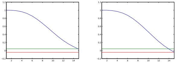
space domains. The correlation functions defined in (7) and (8) were computed and the numerical results are shown in Fig.(1) and Fig.(2).

0 100 200 300 400 500 600 −0.2

0 0.2 0.4 0.6 0.8 1 1.2

0 100 200 300 400 500 600 −0.2

0 0.2 0.4 0.6 0.8 1 1.2

Figure 1: Correlation functions φ(yyt)(τt) (left) and φy(t2)_y2(τt) (right) in (7) cal-culated from Ns = 2000 random data samples of the u-subsystem of the spot replicating system in Example 1

2 4 6 8 10 12 14 −0.2

0 0.2 0.4 0.6 0.8 1 1.2

2 4 6 8 10 12 14 −0.2

0 0.2 0.4 0.6 0.8 1 1.2

Figure 2: Correlation functionsφ(yys)(τs) (left) and φ_y(s2)_y2(τs) (right) in (8) cal-culated from Ns = 2000 random data samples of the u-subsystem of the spot replicating system in Example 1

From the Figs.(1) and (2), the time values when the correlation functions

φyy(t)(τt) and φ_y(t2)_y2(τt) first cut the 95% confidence boundary are 550 and 560 time steps. So we can setτm,t= 550. Similarly, we getτm,s= 14. According to the selection rule (12) and (13) proposed in Section 2.1, the sampling intervals for the spot replicating system in the time and space domains can be chosen between τm,t/20 and τm,t/10. Therefore,Tt is chosen to be 30 which is equal toτm,t/18.3. Similarly, Ts is chosen to be 1 which is equal to τm,s/14. So the size of the spot replicating system for identification is regulated as 50×50×30, where 50×50 is the spatial size that is kept invariant from the original size and 30 is the time which is equivalent to 90/Tt.

replicating system were corrupted with normally distributed noise with a stan-dard deviationσu = 0.0581 and σv = 0.0058. The identification method pro-posed in the previous Section was then applied. The maximum temporal lags and spatial radius were set asnu= 1,nv = 1 andmu = 1,mv = 1. There are three inputs in the regression model (6), ui,j(t), vi,j(t) and u∗i,j(t), where the variableu∗

i,j(t) =ui−1,j(t) +ui+1,j(t) +ui,j−1(t) +ui,j+1(t) is a combination of

the outputs of neighbouring sites to ensure a symmetric topology and a simpler set of candidate model terms. The initial nonlinearity degree of the candidate model terms for identification was set to be 3. The identification results are shown in Table(1). Snap shots of the system output at different times and the model predicted output of the u-subsystem are displayed in the Fig.(3). Note that in this example only theu-subsystem was investigated, so the output of the

v-subsystem is treated as an input during the calculation of the model predicted output of theu-subsystem. The model predicted output of theu-subsystem is defined as

u(_i,jmpo)(t) = ˆf(u(_i,jmpo)(t−1), u∗

i,j

(mpo)

(t−1), vi,j(t−1), vi,j∗ (t−1)) (33)

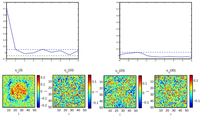
where ˆf(·) is the identified CML model. From Fig.(3), it can be seen that the identified CML model predicts very well and the spot replicating process is closely repeated. The model validation tests were applied to validate the final CML model, where Nv = 1600 samples of data were randomly selected. The results are shown in the Fig.(4). It can be seen that both the correlation functions of model validation tests φβε2(τ) and φ_βu2(τ) fall within the 95% confidence intervals.

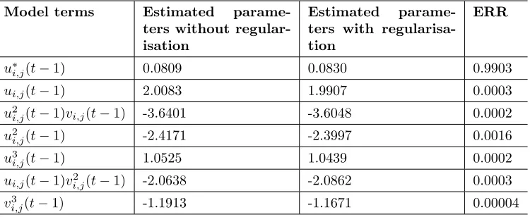
Table 1: Terms and parameters of the identified CML model for u-subsystem in Example 1

Model terms Estimated parame-ters without regular-isation

Estimated parame-ters with regularisa-tion

ERR

u∗

i,j(t−1) 0.0809 0.0830 0.9903

ui,j(t−1) 2.0083 1.9907 0.0003

u2

i,j(t−1)vi,j(t−1) -3.6401 -3.6048 0.0002

u2

i,j(t−1) -2.4171 -2.3997 0.0016

u3

i,j(t−1) 1.0525 1.0439 0.0002

ui,j(t−1)vi,j2 (t−1) -2.0638 -2.0862 0.0003

v3

i u i,j(1) 20 40 10 20 30 40 50 0.2 0.4 0.6 0.8 1 i j u i,j(8) 20 40 10 20 30 40 50 0.2 0.4 0.6 0.8 1 i j u i,j(15) 20 40 10 20 30 40 50 0.2 0.4 0.6 0.8 1 i j u i,j(30) 20 40 10 20 30 40 50 0.2 0.4 0.6 0.8 1 i u i,j(1)

10 20 30 40 50 0.2 0.4 0.6 0.8 i j u i,j(8)

10 20 30 40 50 10 20 30 40 50 0.3 0.4 0.5 0.6 0.7 0.8 i j u i,j(15)

10 20 30 40 50 10 20 30 40 50 0.4 0.5 0.6 0.7 0.8 i j u i,j(30)

10 20 30 40 50 10 20 30 40 50 0.4 0.5 0.6 0.7 0.8

Figure 3: Snap shots of the noisy system output (top) and model predicted output (bottom) at different times for theu-subsystem in Example 1

0 1 2 3 4 5 6 7 8

−0.1 0 0.1 0.2 0.3 0.4 0.5 0.6 0.7 0.8

−8 −6 −4 −2 0 2 4 6 8

0 0.1 0.2 0.3 0.4 0.5 0.6 0.7 0.8 i u i,j(3)

10 20 30 40 50 10 20 30 40 50 −0.2 −0.1 0 0.1 0.2 i j u i,j(10)

10 20 30 40 50 10 20 30 40 50 −0.1 0 0.1 i j u i,j(20)

10 20 30 40 50 10 20 30 40 50 −0.1 0 0.1 i j u i,j(30)

10 20 30 40 50 10 20 30 40 50 −0.1 0 0.1

Figure 4: Correlation functions of the validation tests using the final identified model of theu-subsystem of the spot replicating systems in Example 1, (top left) φβε2(τ), (top right) φ_βu2(τ) and (bottom) some snap shots of the OSA prediction error at different times.

5.2

Turing Patterns

Consider the two-dimensional BVAM (Barrio-Varea-Aragon-Maini) model that is described by the following coupling partial differential equations[2]

˙

u=Du▽2u−η(u+av−Cuv−uv2) ˙

The BVAM model was devised as a formal or phenomenological Turing model and it is not based on any real chemical reactions. The terms uv and uv2

describe the nonlinear inhibition of the activator chemical uby the inhibitor chemicalvwhile the nonlinear termuv2 _{is not included since it would describe}

the reverse behavior. The parameters defining the reaction kinetics were set as

a= 1.112, b=−1.01, η = 0.450,h=−1 and C = 1.57. In this example, the diffusion coefficients were set as Du = 0.516, Dv = 1 so thatDu/Dv < 1 for Turing instability to occur.

The initial concentration distribution corresponds to random perturbations around the trivial stationary state (u0, v0) = (0,0) in the BVAM model with

a variance significantly lower than the amplitude of the final patterns. The boundary conditions for (34) were chosen to be zero-flux in this example. The system size of the BVAM model is 32×32 with a mesh size 64×64. The system was numerically simulated for 192000 steps with the time step set to be 0.05 using the Euler method and the 2nd order spatial derivatives were approximated by the center difference equation. The original data was then down sampled in the time domain from 192000 to 2400 in order to reduce the overhead of computations.

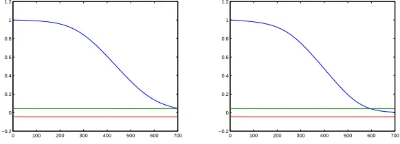
To determine appropriate sampling intervals of the spatiotemporal data for identification, the correlation functions defined in (7) and (8) were calculated. It should be pointed out that the data for the correlation analysis are randomly sampled within the period from t = 0 to t = 1000 in the time domain since the data in this period are used for identification and the remainder is used for prediction tests. The numerical results are shown in Fig.(5.2) and Fig.(5.2).

0 100 200 300 400 500 600 700 −0.2

0 0.2 0.4 0.6 0.8 1 1.2

0 100 200 300 400 500 600 700 −0.2

0 0.2 0.4 0.6 0.8 1 1.2

Figure 5: Correlation functionsφ(yyt)τt) (left) andφ_y(t2)_y2(τt) (right) in (5.1) calcu-lated fromNs= 2000 random data samples of theu-subsystem for the Turing system in Example 2

From the Figs.(5) and (6), the time values when the correlation functions

2 4 6 8 10 12 14 16 −0.2

0 0.2 0.4 0.6 0.8 1 1.2

2 4 6 8 10 12 14 16 −0.2

0 0.2 0.4 0.6 0.8 1 1.2

Figure 6: Correlation functions φ(yys)(τs) (left) and φ(_ys2)_y2(τs) (right) in (5.1)calculated from Ns = 2000 random data samples of the u-subsystem for the Turing system in Example 2

τm,t/10. Therefore,Ttis chosen to be 32 which is equal toτm,t/18.6. Similarly, the sampling interval in the space domain can be chosen betweenτm,s/20 and

τm,s/10. AndTs is chosen to be 1 which is equal toτm,s/14. So the size of the Turing system for identification is regulated to be 64×64×70, where 64×64 is the spatial size which is kept invariant from the original size and 70 is the time scale which is equivalent to 2240/Tt.

The data from the Turing system were corrupted with normally distributed noise with standard deviationsσu = 0.0403 and σv = 0.0058. The maximum temporal lags and spatial radius of the candidate model terms were set asnu= 1,nv = 1 and mu = 1,mv = 1. Similar to the first example, there are three inputs in the regression model (6),ui,j(t),vi,j(t) andu∗i,j(t), where the variable

u∗

i,j(t) = ui−1,j(t) +ui+1,j(t) +ui,j−1(t) +ui,j+1(t) is a combination of the

outputs of neighbouring sites. The nonlinearity degree of the candidate model terms is set to be 3. The final identified CML model for the u-subsystem is shown in Table(1). Fig.(7) shows some snap shots of the system output and model predicted output of theu-subsystem at different times, while the model predicted output of theu-subsystem is calculated in the same way as (33) where thev-subsystem is treated as an input.

The identification data of the Turing system (N= 1600) were sampled from

time and space domain.. The validation test results are shown in the Fig.(9). It can be seen that both the correlation functionsφβε2(τ) andφ_βu2(τ) fall within the 95% confidence intervals. It can also be seen that the correlation tests of the final CML model that was identified with Bayesian regularisation are almost the same as the identified CML using the normal method in this example.

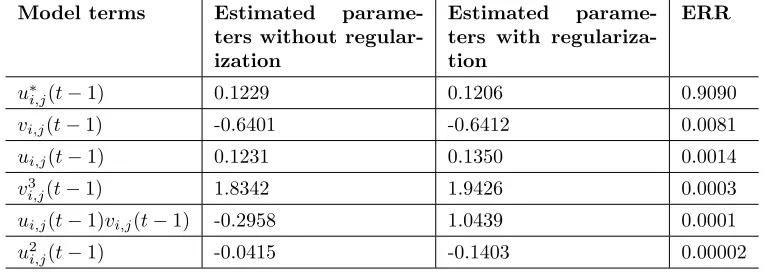
Table 2: Terms and parameters of the identified CML model for theu-subsystem of the Turing system in Example 2

Model terms Estimated parame-ters without regular-ization

Estimated parame-ters with regulariza-tion

ERR

u∗

i,j(t−1) 0.1229 0.1206 0.9090

vi,j(t−1) -0.6401 -0.6412 0.0081

ui,j(t−1) 0.1231 0.1350 0.0014

v3

i,j(t−1) 1.8342 1.9426 0.0003

ui,j(t−1)vi,j(t−1) -0.2958 1.0439 0.0001

u2

i,j(t−1) -0.0415 -0.1403 0.00002

i

j

u

i,j(1)

20 40 60

20 40 60 −0.05 0 0.05 i j

u_i,j(23)

20 40 60

20 40 60 _−0.4 −0.2 0 0.2 0.4 i j u i,j(45)

20 40 60

20 40 60 −0.2 0 0.2 i j u i,j(68)

20 40 60

20 40 60 −0.2 0 0.2 i u i,j(1)

20 40 60

20 40 60 −0.05 0 0.05 i j u i,j(23)

20 40 60

20 40 60 −0.2 0 0.2 i j u i,j(45)

20 40 60

20 40 60 −0.2 0 0.2 i j u i,j(68)

20 40 60

20

40

60 −0.2

0 0.2

Figure 7: Snap shots of the Turing system noisy output (top) and model pre-dicted output (bottom) at different times for theu-subsystem in Example 2

6

Conclusions

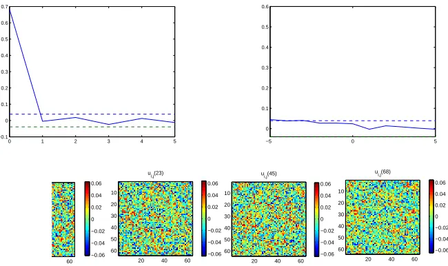
pat-0 1 2 3 4 5 −0.1 0 0.1 0.2 0.3 0.4 0.5 0.6 0.7

−5 0 5

0 0.1 0.2 0.3 0.4 0.5 0.6 60 −0.06 −0.04 −0.02 0 0.02 0.04 0.06 u i,j(23)

20 40 60 10 20 30 40 50 60 −0.06 −0.04 −0.02 0 0.02 0.04 0.06 u i,j(45)

20 40 60 10 20 30 40 50 60 _−0.06 −0.04 −0.02 0 0.02 0.04 0.06 u i,j(68)

20 40 60 10 20 30 40 50 60 −0.06 −0.04 −0.02 0 0.02 0.04 0.06

Figure 8: Correlation functions for the model validation using the final identi-fied model for theu-subsystem of the Turing systems in Example 2, (top left)

φβε2(τ), (top right)φ_βu2(τ) and (bottom) some snap shots of the OSA predic-tion error at different times.

terns has been proposed. Generally, the difficulties associated with the iden-tification of complex spatiotemporal systems depend on the size of the system dimension and the complexities of the underlying dynamics. All of these effects can result in a ill-posed identification problem.

spatiotemporal systems.

7

Appendix

7.1

The OFR Algorithm

For a given candidate set of regressorsG={ϕi}Mi=1 where M is the number of

the candidate regressors, the OFR algorithm can be briefly outlined as follows. Step1: Select the first model term with highestERR

I1=IM ={1,2, ..., M} (35)

wi(t) =ϕi(t),ˆbi= [wi, Y] [wi, wi]

(36)

l1=argmax

i∈I1 ˆ_b2

i [wi, Y]

[Y, Y] =argmaxi∈I1

(ERRi) (37)

w01=wl1, c

0

1=

[w0

1, Y]

[w0 1, w01]

, a1,1= 1 (38)

Stepj, j= 2,3, ...: Iteratively orthogonalise the remaining regressors one by one to select the next model term with highestERRamong the remaining candidate terms.

Ij =Ij−1\lj−1 (39)

wi(t) =ϕi(t)− j−1

X

k=1

[w0

k, Y] [w0

k, w0k]

,ˆbi= [wi, Y] [wi, wi]

(40)

lj=argmax i∈Ij

ˆ_b2

i [wi, Y]

[Y, Y] =argmaxi∈Ij

(ERRi) (41)

w0j =wlj, c

0

j = [w0

j, Y] [w0

j, wj0]

, ak,j = [w0

k, ϕlj]

[w0

k, w0k]

, k= 1,2, ..., j−1 (42)

This procedure is terminated at theMs-th step when a required number of terms in the final model has been selected. The estimated coefficients Θ ={θk}kk==1Ms

associated with the selected terms{ϕlk}

k=Ms

k=1 are computed using

Θ =A−1_{C, (43)}

whereAis upper-triangular matrix which is defined in (16)andC= (c0

1, c02, ..., c0Ms)

is the coefficient vector associated with the orthogonalised terms{w0

k} Ms

7.2

Maximizing the posterior probability with Laplace

pri-ors

Following [12] [11], when W0

is an orthogonal matrix and (W0₎T_(W0_{) = I,}

the solution of the parameterg0

i maximizing the the posterior probability with Laplace priors should be

gi0=sgn(wi0 T

Y)

µ

|wi0 T

Y_{| −} λi ǫ

¶

+

(44)

Letwi=w0ikwik, so thatgi0=gikwik. Replace the wi0and g0i in (44), gives

gi=sgn(wiTY)

µ

|wiTY| −

λi

ǫkwik

¶

+

(45)

References

[1] H. D. I. Abarbanel, R. Brown, and J. B. Kadtke, Prediction in chaotic nonlinear systems: Methods for time series with broadband fourier spectra, Phys. Rev. A41(1990), 1782–1807.

[2] R. A. Barrio, C. Varea, J. L. Aragon, and P. K. Maini,A two-dimensional numerical study of spatial pattern formation in interacting turing systems, Bull. Math. Bio.61 (1999), 483–505.

[3] J. Bascompte and R. V. Sole,Rethinking complexity: modelling spatiotem-poral dynamics in ecology, Trends Ecol. Evol.10(1995), 361–366.

[4] S. A. Billings and L. A. Aguirre,Effects of the sampling time of the dynam-ics and identification of nonlinear models, Int. J. Bifurcation and Chaos5

(1995), 1541–1556.

[5] S. A. Billings, S. Chen, and M. J. Kronenberg, Identification of mimo non-linear systems using a forward regression orthogonal estimator, Int. J. Control 49(1988), 2157–2189.

[6] S. A. Billings and Q. H. Tao, Model validity tests for non-linear signal processing applications, Int. J. Control54(1991), 157–194.

[7] V. Castet, E. Dulos, J. Boissonade, and P. DeKepper, Experimental evi-dence of a sustained standing turing type nonequilibrium chemical pattern, Phys. Rev. Lett. 64(1990), 2953–2956.

[8] D. Coca and S. A. Billings, Identification of coupled map lattice models of complex spatiotemporal patterns, Phys. Lett. A287(2001), 65–73.

[10] P. DeKepper, V. Castets, E. Dulos, and J. Boissonade,Turing type chemical patterns in the chlorite-iodide-malonic acid reaction, Physica D.49(1991), 161–169.

[11] D. Donoho and I. Johnstone,Ideal spatial adaption via wavelet shrinkage, Biometrika81(1994), 425–455.

[12] M. A. T. Figueiredo, Adaptive sparseness for supervised learning, IEEE Trans. Pattern Analysis and Machine Interlligence 25(2003), 1150–1159.

[13] A. Frommer and P. Maass,Fast cg-based methods for tikhonov-philips reg-ularization, SIAM J. Sci. Comput.20(1999), 1831–1850.

[14] G. Golub, M. Heath, and G. Wahba, Generalized cross-validation as a method for choosing a good ridge parameter, Technometrics21(1979), 215– 233.

[15] J. Gradisek, S. Siegert, R. Friedrich, and I. Grabec,Analysis of time series from stochastic processes, Phys. Rev. E62(2000), 3146–3155.

[16] P. Gray and S. K. Scott,Autocatalytic reactions in the isothermal, contin-uous stirred tank reactor - isolas and other forms of multistability, Chem. Eng. Sci 38(1983), 29–43.

[17] , Autocatalytic reactions in the isothermal, continuous stirred tank reactor - oscillations and instabilities in the system a+2b-¿3b, b-¿c, Chem. Eng. Sci 39(1984), 1087–1097.

[18] , Sustained oscillations and other exotic patterns of behavior in isothermal reactions, J. Phys. Chem. 89(1985), 22–32.

[19] L. Z. Guo and S. A. Billings, Identification of coupled map lattice models of stochastic spatio-temporal dynamics using wavelets, Dynamical System

19 (2004), 265–278.

[20] P. C. Hansen, Analysis of discrete ilposed problems by means of the l-curve, SIAM Rev. 34(1992), 561–580.

[21] K. Kaneko, Spatiotemporal intermittency in coupled map lattices, Prog. Theor. Phys. 74(1985), 1033–1044.

[22] ,Turbulence in coupled map lattices, Physica D18(1986), 475–476. [23] ,Pattern dynamics in spatiotemporal chaos pattern selection, diffu-sion of defect and pattern competition intermittency, Physica D34(1989), 1–41.

[25] P. Kareiva and U. Wennergren,Connecting landscape patterns to ecosystem and population processes, Nature 373(1995), 299–302.

[26] M. E. Kilmer and D. P. O’Leary, Choosing regularization parameters in iterative methods for ill-posed problems, SIAM J. Matrix Analysis and Ap-plications 22(2001), 1204–1221.

[27] K. J. Lee, W. D. McCormick, Q. Ouyang, and H. L. Swinney, Pattern formation by interacting chemical fronts, Science16(1993), 192–194. [28] K. J. Lee, W. D McCormick, J. E. Pearson, and H. L. Swinney,

Experi-mental observation of self-replicating spots in a reaction-diffusion system, Nature 369(1994), 215–218.

[29] I. Lengyel and I. R. Epstein,Modelling of turing structures in the chlorite-iodide-malonic acid starch reaction system, Science 251(1991), 650–652. [30] F. Lesmes, D. Hochberg, F. Moran, and J. Perez-Mercader,Noise-controlled

self-replicating patterns, Phys. Rev. Lett.91(2003), 238301–(1–4). [31] D. MacKay, Bayesian interpolation, Neural Computation 4 (1992), 417–

447.

[32] P. K. Maini, K. J. Painter, and H. N. P Chau,Spatial pattern formation in chemical and biological systems, J. Chem. Soc., Faraday Trans.93 (1997), 3601–3610.

[33] S. Mandelj, I. Grabec, and E. Govekar,Statistical approach to modelling of spatiotemporal dynamics, Int. J. Bifurcation Chaos17(2001), 2731–2738. [34] P. Marcos-Nikolaus, J. M. Martin-Gonzalez, and R. V. Sole,Spatial

fore-casting detecting determinism from single snapshots, Int. J. Bifurcation Chaos12(2002), 369–376.

[35] J. L. Maron and S. Harrison, Spatial pattern formation in an insect host-parasitoid system, Science 278(1997), 1619–1621.

[36] C. B. Muratov and V. V. Osipov,Static spike autosolitons in the gray-scott model., J. Phys. A: Math. Gen.33(2000), 8893–8916.

[37] J. D. Murray,Mathematical biology, Springer-Verlag, 1989.

[38] Y. Nishiura and D. Ueyama,A skeleton structure of self-replicating dynam-ics, Physica D130(1999), 73–104.

[39] S. Ostavik and J. Stark, Reconstruction and cross-prediction in coupled map lattices using spatio-temporal embedding techniques, Phys. Lett. A247

(1998), 145–160.

[41] K. J. Painter,Modelling of pigment patterns in fish, In Mathematical Mod-els for Biological Pattern Formation, IMA Volumes in Mathematics and its Applications121(2000), 59–82.

[42] Y. Pan and S. A. Billings, Model validation of spatiotemporal systems by using correlation function tests, Submitted for publication.

[43] U. Parlitz and C. Merkwirth,Prediction of spatiotemporal time series based on reconstruction local states, Phys. Rev. Lett.84(2000), 1890–1893. [44] J.E. Pearson,Complex patterns in a simple system, Science16(1993), 189–

192.

[45] M. T. Rosenstein, J. J. Collins, and C. J. De Luca, Reconstruction ex-pansion as a geometry-based framework for choosing proper delay times, Physica D73(1994), 82–98.

[46] A. Rovinsky and M. Menzinger,Interaction of turing and hopf bifurcation in chemical systems, Phys. Rev. A46 (1992), 6315–6322.

[47] R. Tibshirani, Regression shrinkage and selection via the lasso, J. Royal Statistical Soc. (B)58(1996), 267–288.

[48] R. D. Vigil, Q. Ouyang, and H. L. Swinney,Turing patterns in a simple gel reactor, Physica A 188(1992), 17–25.