Adaptive control of a synchronous generator

ADAPTIVE CONTROL OF

A SYNCHRONOUS GENERATOR

BY

PIYASMI DISSANAYAKA

A report submitted in fulfilment of the

requirements

for the degree of master of technology

in

Department of Electrical & Electrical Engineering

University of Tasmania

Australia

Supervisor

Mr. G. The'

ABSTRACT

This report presents an investigation of adaptive control of synchronous generator

using both a computer simulated model and a laboratory based power generating

system. The outcome of the investigation is encapsulated in computer programs

ACKNOWLEDGMENTS

I wish to thank my supervisor Mr. G The' for his suggestions and the clever guidance throughout this investigation. I also like to thank Mr. B Whettett for his support in the laboratory experiments.

TABLE OF CONTENTS

Page

1. Introduction 1

2. Adaptive control

2.1 General. 3

2.2 Self oscillating adaptive systems. 5

2.3 Gain scheduling. 6

2.4 Model reference adaptive systems. 7

2.5 Self tunning regulators. 8

2.6 Selection of sampling time 11

2.7 Application of anti-aliasing filter 12

3. Computer simulation of synchronous machine.

3.1 General. 13

3.2 System equations of 30MW alternator. 15

3.3 Open loop system 16

3.4 System identification

3.4.1 System model. 18

3.4.2 Time varying parameters. 21

3.4.3 Parameter tracking. 22

4. Controller design and implementation

4.1 General. 23

4.2 Pole zero placement design. 24

4.3 Design specifications 33

5. Laboratory based power generating system

5.1 Laboratory set up 43

5.2 Adaptive exciter controller 47

5.3 Non-adaptive exciter controller 50

6. Conclusion 53

References 55

Appendices

1. Simulation model of turboalternator 56

2. Recursive least squares method. 61

3. Runge Kutta method. 64

CHAPTER 1

INTRODUCTION

Development of computer technology and modern control theory can be linked to achieve better solutions for the control problems. It is possible to propose high performance alternatives for conventional governor and excitation controllers for a synchronous generator. This investigation is based on a design and implementation of an adaptive exciter controller for a synchronous alternator. The study is extended to identify the feasibility of a combined power and exciter adaptive controllers with a computer simulation.

Primary function of the automatic voltage regulator (AVR) of an alternator is to maintain constant operating terminal voltage. In practice this is achieved by adjusting the generator excitation to suit the varying operating conditions of the machine. Alternators in the power system are non-linear systems that are frequently subjected to random load variation with different magnitudes. Fluctuations in the operating conditions eventually make considerable changes in the system dynamics. Hence the conventional fixed gain AVR becomes degraded in performance when the system moves away from the normal operating point. In general, those controllers are tuned around an operating point and operated linearly within limited range. This off tuning can be successfully tackled by the adaptive self tuning controllers.

This report is organised as follows.

3. The simulation uses fourth order Runge Kutta integration _{to solve non-linear} system equations, derived using Park's algorithm _{for synchronous machines. The} model is tested for its step response by conducting an open loop simulation. Synchronous generator is identified as a plant with a second order discrete transfer function using the recursive least squares method _{with an} Exponential forgetting factor 0.97.

Chapter 4 explains the design and implementation of the control system using the

pole zero placement _{method based on the computer simulated model in Chapter 3.} Together with the adaptive exciter controller, a governor controller is implemented at different operating conditions assuming they are independent of each other.

A laboratory based 7.5KVA synchronous alternator driven by a variable speed DC drive is used for the real time simulation. Implementation of the controller and the hardware set up for the experiments are discussed in Chapter 5. The data acquisition system supplied by BOSTON Technology is used to interface the computer and the remaining sub systems attached to the machines. Chapter 5 also contains a discussion based on the performance of adaptive and non-adaptive controllers implemented.

CHAPTER 2

ADAPTIVE CONTROL

2.1 General

Adaptation means the persistent change of behaviour of a system to cope with

new circumstances. In industrial control, adaptive regulators are designed so that

they can modify their behaviour in response to changes in the dynamics of the

process and the disturbances. At present, ordinary feedback controllers are

successfully operated in most of the control systems. The question arises why

adaptive control becoming more popular. If it is investigated from a practical

view point it is likely that better performances can be achieved.

The concept of adaptive control originated primarily with the aerospace problems.

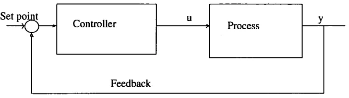
It was found that the classical linear controllers ( Fig 2.1) did not always give

satisfactory control of the altitude of aircrafts. Response characteristics of these

controlled processes varied significantly in flight, and the classical controller could

be matched only to a single flight condition. There seemed to be a need for a

more intelligent controller which could automatically adjust the changing

characteristics of the controlled process. Later it was recognised that such

controllers have valuable features applicable for industrial process control.

It is necessary to investigate the distinction between adaptive control and other

feedback controls. Ordinary feedback controllers adjust the plant states with

reference to fast time scale. Adaptive controllers adjust the plant states with a

feedback reference to a slower time scale for updating the regulator parameters. In

other words, slowly changing states are viewed as changes in parameters.

Regulators with constant parameters are not adaptive because the parameters are

Set poi t

Controller _Process

Feedback

Fig 2.1 Ordinary feedback control system.

It is difficult to decide when adaptive control is useful. There are several reasons

why this should be so. One main reason is that all controlled processes for which

adaptive control might be suitable are essentially both non-linear and stochastic

which is difficult to control and analyse. If they are not non-linear and stochastic

there would be no need for adaptation. Non-linear stochastic problems are difficult

to control by classical control methods because by definition, there can be no

general analytic solutions for them.

It was found that a fixed parameter controller work well in one operating

condition that is tuned, but changes in operating conditions may cause difficulties.

Changes in the plant may create unstable poles and zeros in the transfer function

which may drive the system into unstable situations.

For several decades a wide range of research has been done to implement adaptive

controllers using different approaches. Presently, controllers are designed and

implemented in discrete time rather than continuous time using latest technologies

in sampled data acquisition systems.

4

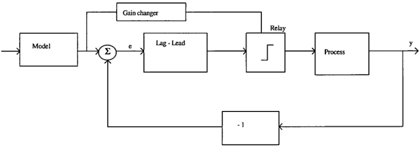
Lag-Lead Model

Process Gain changer

Rela

There are four different approaches of adaptive control commonly used in the industry. However the latter two methods are the only approaches matching with most definitions of adaptive control.

1. Self- oscillating adaptive systems. ( SOASs ) 2. Gain Scheduling.

3. Model reference adaptive control. ( MRAS) 4. Self tuning regulators. ( STRs )

These techniques are discussed in the following sections.

2.2 Self oscillating adaptive systems

Fig 2.2 Self oscillating adaptive system

The frequency of oscillation is influenced by a lag-lead compensation network. Such oscillation creates intentional perturbations in the adaptive system, while exciting it all the time. Then the response of the close loop system is relatively insensitive to variations in the process dynamics. The output signal y, follows the reference input over a certain bandwidth defined by the process dynamics. The model gives desired performance for the feedforward path.

2.3 Gain scheduling

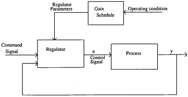
Gain scheduling ( Fig 2.3 ) is viewed as a feedback control system in which the feedback gains are adjusted by means of a feedforward compensation. It is rather an open loop adaptation, by monitoring the operating conditions. Selection of the scheduling variables is based on the knowledge of the physics of the system. There is no feedback from the performance of the close loop system that compensates for an incorrect schedule. It would be rather difficult to find the scheduling variables which reflect the operating conditions of the plant. The inputs to the gain schedule are some of the auxiliary measurements of the plant. When scheduling variables are known, the parameters are calculated for different operating conditions.

Regulator

Parameters Gain Schedule

Operating condition

Regulator Command

Signal

Control Signal

Process

The regulator is calibrated for each operating condition and the performance of each condition is checked by simulations. This method has advantages in some cases because the regulator parameters can be changed very quickly in response to process changes.

2.4 Model reference adaptive systems ( MRAS )

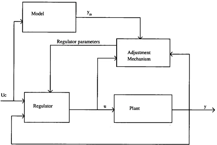
Model reference adaptive systems (Fig 2.4 ) were originally developed to design controllers in which the specifications are given as a reference model . The reference model tells ideally, how to respond to the command signal. The reference model is in parallel with the plant rather than in series. If the error between the reference signal and the feedback

Model

Regulator parameters

Adjustment Mechanism

Uc

Regulator _Plant

Fig 2.4 Block diagram of a model - reference adaptive system.

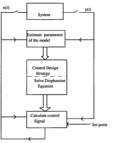
2.5 Self tuning regulators ( STR s)

All the above adaptive methods are direct methods where, the adjustment rules tell directly how the regulator limit should update. SIR is considered as an indirect method where regulator parameters are updated indirectly by parameter estimation and design calculation. Hence MRAS can be treated as a deterministic problem and that the SIR is a stochastic control problem. Some of the principals are the identical for both MRAS and SIR.

STR with explicit identification

The explicit self tuner is designed in such a way that the parameters of the plant are estimated separately with on line calculation of controller parameters corresponding to those estimations. Implementing STR with explicit identification ( Fig 2.5) consists of four steps.

1. Plant parameter estimation scheme to update linearised plant parameters 2. Desired close loop model ( Specifications for the design ).

3. Controller design procedure. 4. Implementation of control law.

These steps are described in Chapter 4 on Controller Design.

System

y(t) u(t)

Estimate parameters of the model

J

Strategy Solve Diophantine

Equation

Calculate control Signal

Set point

Fig 2.5 Self tunning control with explicit identification.

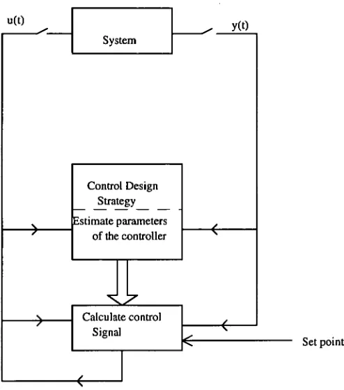
STR with implicit identification

Implicit schemes are first introduced by Astrom and Wittenmark( 1973 ) with an objective of reducing extra computation in identification and control in STRs. In

System

u(t) _y(t)

Control Design Strategy Estimate parameters

of the controller

LI

Signal

Set point

Fig 2.6. Self tunning control with implicit identification.

2.6 Selection of sample time

Selection of sample time is also an important issue in a discrete data system. Too

long sampling periods will make it impossible to reconstruct the continuous time

signal. Too short sampling time will increase the load on the computer. Sampling

time influences properties like; following the command signal; rejection of load

disturbances; and measurement noise . As a rule of thumb sampling interval is

chosen as,

cooh = 0.1 - 0.5

coo is the natural frequency of the dominant poles of the close loop system.

The choice of the sampling time also determines whether an anti aliasing filter would be taken into account in the design. If the desired crossover frequency of the close loop system is close to the Nyquist frequency then it is not desirable. Increasing sampling time eventually increases the order of the model.

2.7 Application of anti-aliasing filter.

CHAPTER 3

COMPUTER SIMULATION OF SYNCHRONOUS MACHINE

3.1 General

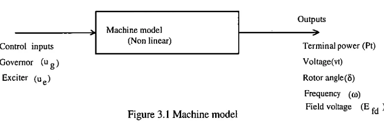
The purpose of the simulation is to validate the controller design before adopting it to a real system. To achieve this objective, a hypothetical synchronous machine is modelled on a computer. The machine model has its inputs and outputs as in Fig 3.1

Machine model (Non linear)

Outputs

Control inputs

Governor (u _g)

Exciter (ue)

Terminal power (Pt)

Voltage(vt)

Rotor angle(8)

Frequency (0)) Field voltage (E fd ) Figure 3.1 Machine model

X= [ 8 ,

ö, w

fd

U = [U„ Ug ] (3.2)

Y =[P, ,v„ 8, E fd ] 7. (3.3 )

X = State vector ( Xe R6 )

U = Input control vector ( U E R2 )

Y = Output measurement vector ( Y E R4 )

Appendix 1 defines all other state variables mentioned above.

Limiter Integrater _Limiter I/T

Governer Set opint

1/(1-1:c s)

Exciter Set point

Control valve

Turbine

1/(1+1j s) Limiter

GT

Vt imp Generator Line

■

1--

■ ■

Infinite Bus

GT = Generator transformer

Figure 3.2 Open loop turbogenerator system

The output vector is chosen in such a way that its elements real power output,

machine terminal voltage, rotor angular velocity and field voltage are readily

accessible for measurement in a full scale plant. The governor input and the

input control vector. Measurement difficulties exist for some of the variables

defined in the state vector. For example, it is difficult to measure rotor angle and

field flux linkage. Output predictions can be estimated in terms of input control

signals and the past output measurement signals, and it should avoid the reference

to any of the state variables. In other words, the plant can be completely defined

by the known and measurable vectors rather than unknown state vectors.

3.2 System equations for 30MW Turboalternator

From Appendix 1, The system equations may be written as the following set of

first order non-linear equations.

kI=X2 ( 3.4 )

X2 = [(x6 -1.256* X3 * sin(X1)+0.922*sin(X1)*cos(X0-0.08*X2]*29.637 ( 3.5 )

k3= 0.180726*X4— 0.561* X3 +0.422*cos(Xt) ( 3.6 )

ka =(—X4+Ui)*10 (3.7)

ks = (—X5+ Kv) * 10 (3.8)

The outputs Y1 and Y2 may be expressed in terms of state variables by,

Yi =1.256* X3 * sin(X0 — 0.922*sin(X0*cos(X0

Y2= + vq2 )"2

where,

Vd = 0.798* sin(X0

vg = 0.59* X3+ 0.361*cos(X0

It is rather difficult to obtain an analytical solution for the above equations 3.4 to

3.9, to calculate the components of the state vector. The Runge Kutta procedure described in Appendix 3, can be used to approximate the solutions of these state

equations by selecting the integration step as 0.005 secs.

3.3 Open loop system

The Open loop test is necessary to check the step response of the model with the

pre assigned initial steady state conditions. A 12% change in real power from 0.8

p.u. to 0.9 p.u. is considered as the step change to the simulator. The increase in

power changes the exciter voltage and the governor input which can be calculated

from the steady state conditions derived from state equations. The step inputs to

the machine are represented by the new steady state control inputs.

Initial steady state conditions :

Xss= [1, 0, 1.152, 2.314, 0.8 , 0.8 ] T

Yss= [ 0.8 , 1.105 , , 2.314]

Uss = [ 2.314 , 0.563 ]

With the step increase of the input control vector, Uss=[ 2.314 , 0.563 1 , the

1.1 1.1 1.1 1.1 1.1 0 Term ina l vo ltag

e p

u

1 2

0.8 0

4.0 —

ro

to

r ang

( deg ) 3.0 — 2.0 — 1.0 — Terminal power Term ina l p ower (p u ) 0.9 0.8

0 2

Time(sec) Terminal, voltage 3 time (sec) Steam power 1.0

1 2 3

time (sec)

5.0 Rotor angle

0.0

0 2

time (sec)

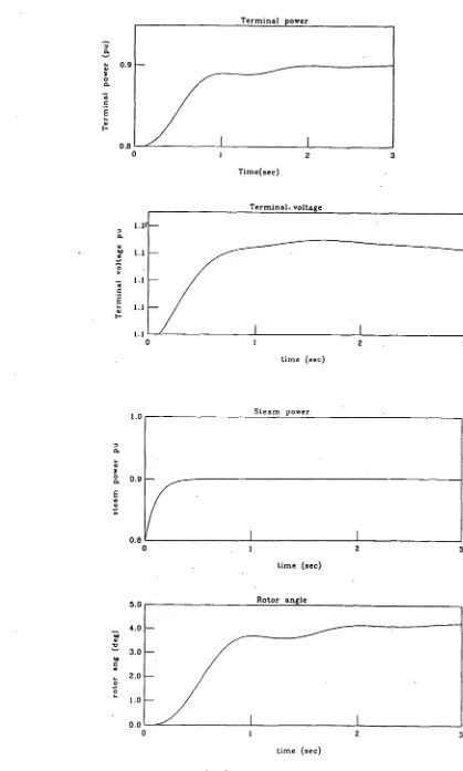
Fig 3.3 Open loop characteristics of the turboalternator

New steady state conditions :

U„=[ 2.314 , 0.563 1

Xs,. [ 1.078, 0, 1.160, 2.495 , 0.9 , 0.9 11. Y„. [ 0.9 , 1.109 , 0 , 2.495]

Open loop simulation was conducted using the solutions of the Runge Kutta integration formula. Open loop simulation uses the computer program listed in Appendix 4.

Fig 3.3 shows the performance of the open loop system. These open loop results have proved that control laws can be applied to design a stable close loop system.

Fig 3.3.a indicates the terminal power variation against time for the step increase of control inputs. A slower governor creates a significant time lag in terminal power compared to the steam power represented by Fig 3.3.b Fig 3.3.c and Fig 3.3.d which indicate the change in rotor angle and terminal voltage due to the step input.

3.4 System identification

3.4.1 Model:

The turboalternator system is modelled by a second order discrete transfer

function,

biz-' +b2z-2 Y(z 1 )

G(z)= =

1+ale +a2C2 U(z 1 ) ( 3.12 )

where Y and U refer to the output and input vectors of the system. Parameters

1) 1 , b2, al , a2 describe the dynamic behaviour of the plant as in the equation 3.12.

Obtaining the inverse transform of equation 3.12, it can be represented as,

yk = bl Ilk - I ± b 2 Ilk - 2 — al yk - I — a2 yk- 2 ( 3.13 )

Equation 3.13 is a difference equation representing the previous sample values of

the input and output that is been used to predict the next output sample. It is a

recursive equation, and can be calculated using identified parameters b 1 , b2, at , a2

x1J Input ] _y

k [ output ]

Unknown system

) 1 + a /z + a /zsz

1 2 b _I/z + b

2 /z*z

Model v _{ek [ Error signal ]}

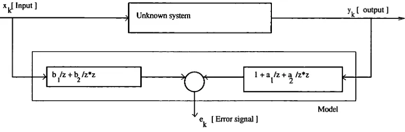
Fig 3.4 System identification process

The error signal generated from the model denoted as ek is given by,

ek= yk—bluk -1— b2uk - 2 +auk -1+ auk - 2

In matrix form, Y = HO + e

where H and 0 are vectors given by, H = [ Uk - I Uk - 2 yk - I yk - 2 ]

0 T = [bi bz -al -a2}

Y is the observed variable vector, whereas H represents known function values

consisting of past measurements and control signals that are often termed as

regression variables, and 0 represents the unknown parameters. The error vector e

is to be minimised to obtain the optimal solution for the parameter vector 0. As

described in Appendix 2, this matrix equation is solved using the least squares

method while minimising the squares error represented by the loss function J.

The solution for 0 is updated in every sample recursively, and implies that the

3.4.2 Time varying parameters.

In the least square method, the parameters are assumed to be constant throughout

the whole time period. Adaptive control problems are such that the parameters

are time varying by nature. The case of parameters that are slowly varying can

be simplified to a mathematical model[I] . it is by replacing least square criterion by

1 i

j . _7 8 tk ( y k ... HT 0 )2 2 IT'

where the parameter 8 lies between 0 and 1, and 8 is termed as Exponential

forgetting or discounting factor. The loss function in the above equation implies that the time varying weighting of the data of the data is introduced. The latest

data is given a unit weight whereas k time units old data is given a weighting of 8

k. In practice the most suitable value for the exponential forgetting factor lies between 0.9 and 1. When 8 =1 , the weighting no longer exist in the least square

estimation.

To give the late measurements more weight than the earlier measurements an exponential forgeting factor is applied in the formulae A 2.4, A2.5, A2.6 . It is represented as,

A

Oki.' = eAk ± Kk+I(Yk+1 — Hk+i eAk ) (3.14) and,

Pk+I = (Pk — K k+11-1k+IPk) I 8 (3.15)

where,

Kk+i = Pk Hk7,"( 8 + Hk+1 Pk H kT+1) -1 (3.16)

The design is crucial with system identification. Excessively fast discounting may

cause the parameters to be uncertain and excessively slow discounting will make it

3.4.3 Parameter tracking

The ability to track the time varying process parameters effectively is a key issue and a highly desirable property of an adaptive system. The parameter tracking capability depends on the least squares covariance matrix P. Elements of P determine the rate of parameter tracking. These estimators tend to decay to small values rather rapidly. As a consequence, the ability of tracking parameter variation is quickly lost. To improve tracking performance the covariance matrix diagonal elements are to be reset if the trace is very small.

Updating the parameters of the covariance matrix P is possible at different set points, by applying the Constant trace algorithm. _{This can be done by ensuring} the trace of P constant at each iteration. The constants of resetting, has a practical value, but is a function of noise and is experimentally selected for the most suitable response.

CHAPTER 4

CONTROLLER DESIGN AND IMPLEMENTATION

4.1 General

This chapter is mainly focused on the close loop system that involves controller design based on estimated parameters of the synchronous generator model in Chapter 3. The close loop system should be viewed as an automation of process modelling and design in which the process model and controller are updated at each sampling period.

The synchronous generator modelled in Chapter 3 satisfies the open loop performance of the system that enables it to apply the control law as desired. The implementation of a self tuning controller is based on the pole zero placement approach proposed by Astrom and Wittenmark(1980).

Set point

Design

Regulator

Identification

Plant

I

Output

Fig.4.1 Block diagram of SISO(single input single output) Adaptive control system

There exists a difference between tuning and the adaptation process. In tuning, it is assumed that parameters are constant, whereas in adaptation it is assumed that parameters are changing all the time. Therefore to cope with these basic principles in self tuning adaptive problems, it is assumed that the parameters are changing slowly.

4.2 Pole Zero placement Design.

Consider a process with one input u, and one measured output y, which are related by the transfer function, H(z) ,

B (z-1 ) H (z-1)= Z-k

A (z -1 )

where A(z -1 ) and B(z 1 ) are polynomials. z-' is backward shift operator. A and B are relatively prime , e., that they donot have any common factors. Further it is assumed that A is monic , i.e., the coefficientof the highest power in A is unity.

( 4.1 )

A (z ) = 1 +al z-1 +a2C2 B (z-`)= b1z-1 + b2C2 k > 0

The pole excess is defined as d = deg A -deg B, and is the time delay in the process in discrete time systems. Parameters a l , a2, b 1 and b2 are estimated by the

G.(z-1 ) = Z—k Bin (Z I ) ( 4. 2 )

A. (CI )

where A. and B. are co - prime and monic . For stability, the zeros of A. should be inside the unit circle.

It is not sufficient to specify Gm as the close loop characteristics. With output feedback, there will be additional dynamics that are not excited by the command signal. i.e., the observer dynamics are not controllable from the reference signal. Hence it is necessary to specify the observer dynamics. This is done by specifying the characteristic polynomial Ao as the observer. It influences the sensitivity to load disturbances and measurement.

As discussed by Wittenmarkm(1980), two main assumptions need to be taken into account in specifying a close loop model. Firstly, it is assumed that the delay in the desired close loop model is at least as long as that in the open loop model. Secondly specifications must me such that unstable or poorly damped process zeros must also be zeros of the desired close loop transfer function.

A general linear regulator proposed by Astrom and Wittenmark[I], is described as,

Ru = T. uc -S y

where u , uc and y represent the input to the process, controller set point and process output respectively. R, S and T are polynomials in discrete domain.

Uc

Plant

B k

A

Set point 1/R

y Output

Fig 4.2 represents the close loop control system with the linear regulator. The

close loop equation can be written as,

R(z-1 )U ) = T(z-I )U,(z)— S(z-I )Y(z 1)

Then the close loop transfer function relating y and u c is given by,

z _k TB ( 4.3 )

AR+ z-k BS

To carry out the design the ploynomial B is factorised as B = B+ . B- where B+

is a monic polynomial whose zeros are stable (inside the unit circle ) and so well damped that they can be cancelled by the regulator. When B+ =1 , there is no cancellation of any zeros .

Controller

Fig 4.2 Self tunning regulator

To achieve the desired input and output response, the following condition 4.4

From equations 4.2 and 4.3,

BT _.

(4.4) AR+BS Am

The factors of B that are not also factors of B. must be factors of R. Factors of B which correspond to close loop zeros, should be cancelled if not desired.

To get a causal controller the close loop model in equation 4.2 must have the same or higher pole access as the process in equation 4.1.

This give the condition,

deg A. - deg B. ... deg A - deg B ( 4.5 )

Considering the polynomial equalities , the denominator of equation 4.4 becomes, AR

Since B+ is cancelled it is also factors of close loop polynomial ,

AR +. B - .S = Am .A0

Equation 4.6 is called Diophantine equation. Where R = 12' B+ . B+ has been cancelled off.

The numerator of equation 4.4 can be written as, T = Ao.B„, I B -

(4.6)

(4.7)

( 4.8)

The solutions of the above equations ( 4.7 ) and ( 4.8 ) can be justified by considering the constraints for the degree of each polynomial.

The conditions,

deg R deg T ( 4.9 )

ensure that the feedback and feed forward transfer functions are causal. If the time to calculate the control signal in the computer is only a small fraction of the sampling period, then it is acceptable to assume,

deg S = deg R = deg T ( 4.11 )

If the computation time is close to the sampling period the corresponding relation becomes,

deg R = 1 + deg T = 1 + deg S (4.12)

This means that there is a time delay in the control law of one sampling period. From equation ( 4.5 )

deg Am - deg Bn, ?. deg A - deg B

deg AR = deg (AR +BS ) = deg B+ A. Am

deg R = deg A0+ deg Am + deg B+ - deg A From 4.8,

deg T = deg A.+ deg B- deg B-

It can be shown that, there exists a solution for the Diophantine equation when, deg S < deg A

Choosing deg S = deg A -1, and Since deg R deg S , from equation 4.9, deg A0+ deg Am + deg B+ - deg A deg A -1

deg A. 2 deg A -deg Am - deg B+ -1 (4.13)

Equation 4.13 can be used to obtain the degree of the observer polynomial A.. This condition implies that the observer polynomial is sufficiently high to ensure the causality of the control law. It should be stable and fulfil the compatibility conditions.

Open loop transfer function,

H(z)= = Ki 2 Z(Z + b)

A +a,z+a2) where K1 = 61 and b = b2 I b,

if b <1 then 13- =K and 13+ = (z + b)

if b >1 then 13- = K, (z + b) and 13+. = 1

( 4.14 )

The value of b represents the open loop zero that can lie inside or outside the unit \

disc. If the zero is inside the unit disc it should be cancelled in the close loop

system. If the zero is outside the unit disc, the zero should be included in the close

loop because unstable zeros cannot be cancelled. Both cases are separately

described for the specific design in this simulation.

Case 1: b<1.

The close loop transfer function is assumed as,

G.(z)=z (21+p, +p2) B„,

+p1.z+p2) An,

Open loop transfer function is given by ,

H(z)= —B = K, . 2 Z(Z b)

A (z +a,z+a2) where Ki =b1 and b = b2 I 61

Because b <1 , 13- = Ki

13+ = (z + b)

By considering the degrees of (4.14) and (4.15),

deg A =2 ;

deg B =2 ; deg A,,, =2 ; deg B„, =1 ; Hence,

degS = deg A-1 = 1;

deg R = 0 ; deg Ao ?_0; deg T = 1;

Let, S = So z + SI

T=To z+T, .

I?' = Ro z+ RI

Equating the close loop system reference to equation ( 4.4 ),

BT ₌

AR+BS Am

Then,

b1(T0z+71)=(1+p1 +p2)z

T, =0;

l+pl +p2

To =

bi

Similarly considering the denominators,

(z2 +a1 z+a2 )(R0z+RI )+(S0 z+SI )b1 = (z2 +p1 z+p2 ) R1 =0;

Ro = 1;

So =(p, —a, )/b1 ;

SI = (p2 —a2)/ b, ;

R=(z+b).1

The control law can be written as, RU = TUc - SY

(z+ b)U = Toz.0 c — (So z + SI )Y

Converting into a difference equation by taking inverse z transform,

Case 2: b>1.

Since b>l, the zero cannot be cancelled in the desired response. Therefore b should be included in the desired close loop transfer function. To achieve unity gain throughout the control loop, the expression for the transfer function is divided by (l+b).

Then the desired response is given by,

(z+

G () b) (l+p, +p2) . B,,, (l+b)(z 2 +191.z+ p2) A. Open loop transfer function in equation 4.14,

H(z) =13-- = K,. 2 Z(Z ± b)

A (z + alz+ a2) where K1 =b1 and b = b2 I b,

Because b > 1 then 13- = KI (z + b) and B+ = 1

By considering the degrees of (4.14) and (4.15), deg A =2

deg B =2 ; deg An, =2 ; deg B,„ =1 ;

Hence,

deg S = deg A -1 = 1; deg R = 1;

deg Aoa); Let, deg Ao =1;

deg T = 1;

Let, S = Soz + SI

T =Toz+Ti

R. = Roz+ RI .

Ao = z

Equating the close loop system reference to equation ( 4.4 ),

BT B₌ m

A R+ B S Am

Then,

b1(T0z+7j)=(1+PI ±P2)/(1+b)

T, =0;

1+ 131+ 132

To =

- b1(1+ b)

Similarly considering the denominator,

(z2 + alz+ a2)(Roz+ R1 )+ (z+ b)(Soz+ SI)b, = z(z2 + Piz+ P2)

Ro =1;

RI = b b.(b2 — plb+ p2)

(b2 —alb+ a2)

So = (p1 —a1 — R1)1 bi ;

SI = —a2R, 1 b2;

R=z+R1

The control law can be written as, RU = TUc - SY

(z+ RI )U = Toz.U, —(Soz+ SOY

Converting into a difference equation by taking inverse z transform,

Irrespective of the location of the close loop zeros, the control law remains valid, since low frequency steady state gain of the desired close loop system is maintained as unity.

4.3 Design specification :

The specification of the close loop transfer function needs to include the process zeros and poles. Specifications of all poles and zeros for a higher order system require more parameters. It rarely makes sense in practice to give so much data. It is more desirable to give some global characteristics, such as dominant poles in desired dynamics.

A discrete time system can be specified only to include the dominant poles by selecting Am as,

= 1 — 2.e°" .cos(c0.11 c2 ). z-I = (z2 prz p2 )z-2

where,

= Damping coefficient. h = Sampling interval co = Resonance Frequency.

pi , p 2 are the parameters defined according to equation4.19.

Equation ( 4.19 ) corresponds to a second order continuous time process with damping C and frequency of resonance co sampled with period h. It is often easy to select C and co such that the system gets desired properties. The damping ratio is often chosen in the interval 0.5 - 0.8. The resonance frequency co, is chosen by considering the required rise time and the solution time.

4.4 Simulation

The Simulation uses the least squares identification and Runge Kutta integration from the previous Chapter and the designed controller for given specifications. In the implementation of the exciter controller, the exciter close loop is assumed as having following specifications.

Resonance frequency : 4 Rai's Damping ratio 0.7

sampling time 0.05 Second

Similarly, in the implementation of governor controller, governor close loop is assumed as having following specifications.

Resonance frequency : 1 Rad/s Damping ratio 0.9

Simulations are conducted at four distinct system conditions. 1. Adaptive exciter control with fixed governor setting. 2. Non adaptive exciter control with fixed governor setting 3. Adaptive exciter controller with adaptive governor controller. 4. Adaptive exciter controller with non adaptive governor controller.

Different voltage set points are appropriately set to identify the variation of the output conditions as in the Table 4.1. The simulation was performed for 600 sample values equivalent to 30 seconds The vector notation used in simulations can be listed as follows.

Time(second) 0 -5 5-10 10-15 15-20 20-25 25-30

voltage

set point( p.u. )

1.15 1.22 1.22 1.2 1.33 1.4

Table 4.1

In cases where power controllers are implemented, different power levels are set as in Table 4.2.

Time (Second) 0-12.5 12.5-22.5 22.5-30

' Power set point ( p.u. ) 0.7 0.8 0.95

Table 4.2

Input control vector U = [ ul u2

where u 1 = Exciter control input u2 = Governor control input Output measurement vector

Y = [ yl y2 ]

y2 = Terminal voltage. U = Terminal voltage set point Psp = Terminal power set point.

Start up Procedure

There are several ways of initialising a self tuning controller based on a priori information about the process. However, a practical value is more feasible. In these simulations each parameter is initialised as one at the starting condition. The initial value for the covariance matrix is chosen as 100 times the unit matrix . These values are not critical because the estimator will reach the proper values within a reasonable time. In practice 10 to 50 samples are more than enough for a good controller to track the plant. A perturbation signal is added at the start to speed up the convergence of the estimator. It is often desirable to limit the control signal to a safe value at the start up.

Case 1 : Adaptive exciter controller with fixed governor setting.

set points are changed. The Fig 4.3.c clearly shows how the terminal power behaved with respect to time.

Case 2 : Non adaptive exciter controller with fixed governor setting.

A non adaptive exciter controller was designed from the parameters obtained at a random point of the simulation program for Case 1. The control equation for the non adaptive exciter controller is written as,

Ulk = 1.2423 usp +16.022 y2k, — 15.763 y2 k, -, +O.l869 UlkI

The suffix kl denotes the present sample value and the suffix kl-1,k1-2 denote the previous sample values.

The terminal power set point was remain unchanged at 0.8 p.u. The terminal voltage set point was changed as in the previous case. The computer program FP_NAV.PAS was used to simulate the controller and the operating conditions were recorded for a period of 30 seconds. Figures 4.4.a, 4.4.b and 4.4.c represent the corresponding variations of system states.

It can be seen that from fig 4.4.a, the parameter tracking is not as accurate as the adaptive controller in Case 1.

Case 3. Adaptive exciter and adaptive governor controller.

controller in Case 1. A power controller was also implemented using the same techniques, with a unity exponential forgetting factor _{in the identification. The} computer program ADV_ADP.PAS ( Appendix 4 ) was used for the simulation and the operating conditions were recorded for the period of 30 seconds. The results are plotted in Figs 4.5.a, 4.5.b, 4.5.c.

From the results it is clear that , the combined adaptive and power controller functions better than previous cases (Case 1 and Case 2). Because the governor is adaptive, the power changes reflected due to the set point change of terminal voltage would cause a transient in the governor control input.( Fig 4.5.d ). From figures 4.5.a and 4.5.c proved that the time constant of the governor is comparatively smaller than the time constant of the exciter and the controllers are capable of tracking respective set points.

Case 4. Non adaptive governor and adaptive exciter controller.

The parameters of the governor controller was obtained at a randomly selected point of the simulation in Case 3.

The control equation for the governor control signal was then calculated as, u2k, = 0.195 Psi, _{—1.402 yl ki + 0.671 yl k, _, + 0.1762 u2 k1 _,}

The simulation was conducted with set point variations as in the tables, to implement adaptive voltage and non-adaptive power controller. The results monitored for the period of 30 seconds and are plotted on Figs 4.6.a, 4.6.b and 4.6.c.

Terminal voltage Te rm ina l Vo ltag

e (p

u ) Exc iter Inp u

t (p

u ) 1.4 1.1 1.0 0 5.0 4.0 3.0 2.0 1.0 0.0

Controller Set Point Terminal voltage P9

6 12 18 24

Exciter Input

30

6 12 18 24 30

Termini Power Te rm ina l Po wer (p u

) 1.2

1.0

0 . 8

0.6

0.4

Controller Set Point 0.2

0.0

0 6 12

Governor Input Terminal Power PU 1

18 24 30

Go

ver

nor

Inp

u

t. (p

u

)

0.7

0.5

0.3

6 12 18

Fig 4.3 Characteristics of adaptive exciter controller with fixed power

Controller Set Point Terminal Power PU 1 1.2

0. 1.0

0.8 0.6 0 — 0.4 5 0.2 0.0 Terminal voltage Exc iter Inp

ut (p

u ) Term ina l Vo ltag

e (p

u ) 1.4 1.1 1.0 0 5.0 4.0 3.0 — 2.0 1.0 0.0 0

Controller Set Point

Terminal voltage P1.1

I

6 12 18 24 30

Exciter Input

6 12 18 24 30

Termini Power

6 12

Governor Input

18 24 30

0.7

0.5

0.3

0 6 12 18 24 30

Fig 4.4 Characteristics of Non adaptive exciter controller with fixed power

Go

vernor

Inp

u

t (p

Controller Set Point

Terminal voltage

1.0

— Terminal voltage Pli

o 6 12 18 24 30

Exciter Input 5.0

0.0

0 6 12 18 24 30

Termini Power Term ina l Vo ltag

e (p

u ) 1.4 1.1 1.2 Te rm ina l Powe

r (p

u ) 0.6 0.4 0.8 0.2 1.0 0.0 Go verno

r Inp

u

t. (p

u

)

0.7

0.5

0.3

Controller Set Point Terminal Power PU

6 12 18

Governor Input

24 30

0 6 12 18 24 30

12 18 24 30

0 6

Terminal voltage

Controller Set. point Terminal voltage

. I

Exciter Input Te rm ina l Vo ltag

e (p

u ) 1.0 0 1.4 1.1 5.0

24 30

0, 4.0

0.0

Controller Set Point Terminal Power PU 1 1.2 Term ina l Po wer (p u ) 1.0 0.8 0.6 0.4 0.2 0.0 Termini Power

0 6 12 18 24 30

Governor Input

r3" 0.7

0.5

0.3

0 6 12 18 24 30

CHAPTER 5.

LABORATORY BASED POWER GENERATING SYSTEM.

5.1 Laboratory set up

The simulations conducted in Chapter 4 are designed for a hypothetical machine

model based on Park's equations. The real time power generation systems may

have to face more complicated problems in implementations, especially with

regard to the limitations of the hardware used in the experiments and the

non-linerarities in the plant sub systems.

The following block diagram shows the laboratory set up for the power generating

system used in the experiments.

Infinite bus. DC Motor

Synchronous

Machine _FT

Thron Variable speed Controller

SP

I

I

Summing Amplifier

Computer/PC30

Power Feedback

Voltage feedback SIR

Robicon Field Controller

VTR = Voltage Transducer FTR = Power Transducer SIR = Speed Transducer FT = Ferrenti Transformer

SP = Set point

LOAD

The laboratory model of the synchronous generator consists of a 7.5 KVA direct

coupled motor-generator system. The list of apparatus and hardware needed for

the experiment are listed below.

1. A 7.5 KVA synchronous three phase alternator provided with the infinity bus

connection as required.

2. A DC motor with output power more than 7.5KVA supplied with fixed field

voltage.

3. A thyristor controlled 4 quadrant 380V DC rectifier system, with adjustable

output current by gain control.(ROBICON field controller)

4. A thyristor controlled variable speed DC drive, operated with the tacho

feedback

and power feed back.( THRON controller)

5. An IBM compatible personal computer installed with PC30 -BOSTON

technology

data acquisition system. The real time software (QUINN CURTIS -Turbo

Pascal

version) and the Turbo Pascal compiler along with BGI (Borlands Graphics

interface) should also be installed in the computer.

6. A Power transducer measure up to 10KW with a DC output of 2V (HOKI)

7. A 12 pulse 3 phase voltage transducer, to measure the terminal voltage of the

alternator.

8. An Induction motor load of 5KW ( variable) which is wired through a three

phase

contactor.

The complete demonstration of the control system is programmed using TURBO

PASCAL , together with other associated software.

The software program SYS2.pas implemented in the personal computer is

assigned for the following functions.

1. Construction of the artificial plant parameters according to the least squares

estimation.

2. Sensing of operating conditions of the machine and making the corresponding

tuning of the controller parameters.

4. Initiating disturbances to the analog simulation by step inputs to the exciter

set

point.

5. Recording input and output signals and displaying them on the monitor in real

time.

6. Recording the operating conditions in a data file.

While changing the voltage set point at different intervals, voltage feedback was

( passed through the adaptive controller . The input output requirements of the

controller are handled by using 12 bit AID and D/A converters available with

the PC 30 module, together with a suitable interface to the alternator. The signal

inputs and outputs were sampled with sampling time of 0.1 second, corresponding

to the 10 Hz sampling frequency. Specifications for the adaptive exciter controller

are as follows.

Resonance frequency : 4 Rad/s

Damping ratio : 0.7

The sampling frequency is more than 10 times higher than the resonance frequency

of the exciter control close loop plant. Hence as mentioned in Chapter 2 there is

The turbine is represented by the DC motor whose speed is regulated by an electronic turbine governor simulator. The governor simulator is activated by the power feedback and speed feedback from the system. The signal obtained from the power transducer is inverted and summed with a reference signal before being fed in to the governor controller.

The exciter field controller consists of a four quadrant thyristor rectifier which is activated by the signal output from the D/A converter. The D/A signal is summed with a reference DC signal before being fed in to the ROBICON controller. To input the terminal voltage feed back, an A/D channel is selected on the data acquisition module.

The PC 30 module is capable of conducting digital and analog input output operations via the PC bus to the peripherals. It is compatible with the IBM PC, PC/XT, PC/AT, PS2 series of computers. The data acquisition software supplied with PC 30 consists of a set of real time device drivers callable from common languages like PASCAL, C and FORTRAN. 12 bit AID signal inputs are limited to a full scale of +5 to -5V or 0 to 10V and 12 bit D/A signal outputs are limited to full scale of 0 to 10V or -10 to +10V. Those scales are readily programmable from associated software.

time may have a certain mismatch. However, in the experiment it was of minor importance.

The variation of terminal voltage is monitored using the real time graphics at each 0.1 second at different operating conditions given below.

1.Starting condition.

2. Synchronising the machine via Ferrenti transformer. 3. Loading the machine with inductive load.

4. Isolating the bus. 5. Unloading the machine.

5.2 Adaptive exciter controller

The experiment was conducted in two phases. Firstly, an adaptive exciter controller was implemented using the computer program REAL.PAS. The experiment was conducted for the period of 130 seconds . The exciter input signal and the terminal voltage were monitored throughout the period and recorded in a data file. The power control loop was operated as a linear feedback to the governor simulator.

Terminal voltage set points are varied as is the Table 5.1. The experimental results are plotted in Fig 5.2.a and 5.2.b.

Time (seconds) Voltage set point( p.u.) 1 p.u. =415 V

0-10 0.987

10-20 1.054

20-30 1.085

30-40 0.999

40-50 0.9627

50-60 0.987

60-70 1.054

70-80 0.987

80-90 1.054

90-100 1.085

100-110 0.999

110-120 0.9627

120-130 0.987

130-140 1.054

Table 5.1

0 20 4'0 60 Exciter Input

20 40

fr

Terminal voltage

Con troller Set. Point

Terminal vciltage [1pu=415v] 1.3 Term ina l 0.9 Exc iter Inp u

t. (vo

lts ) 0.7 5.0 3.0 1.0 - 1.0 -3.0 - 5.0

1.3 Terminal voltage

Term

in

al

Vo

ltag

e _1.1

0.9

0.7

70 90

Controller Set Point

--- Terminal vrage ( 1 pu=415v)

110 130

Exciter Input

90 110 130

Time(sec)

Fig 5.2 Laboratory based adaptive controller - characteristics

At the 74 th second, the machine was isolated form the bus, and a voltage transient of a small amplitude was resulted. Due to the slower response of the governor simulator, it consumed a much longer time interval to return to the perfectly tuned conditions. At the 100 th second the inductive load was removed from the machine. From Fig 5.2.b it can be seen that the machine safely retuned to its new operating conditions.

5.3 Non adaptive ( Fixed parameter ) exciter controller.

At the second phase of the experiment, a non adaptive controller was implemented using randomly selected plant parameters from the first phase. The plant parameters are,

b1= -0.00832115 b2 =-0.024447 al =-1.277969

a2 =0.4035884

The controller derived from this plant parameters is,

Ulk = —0.32824 us, —1.821669 y2 ki + 2•230243Y2 + 0.15718 ul = exciter input signal (controller output) sample value

Y2k1 = terminal voltage sample value

u = exciter set point _sp

The computer program FREAL.PAS uses the above equation ( 5.1) to implement the non adaptive exciter controller. The voltage set points were varied similar to the previous experiment. The response obtained by monitoring the controller for the period of 130 second was plotted in Fig 5.3.

1.3 Ter m in al Vo ltag

e (p

u ) 0.9 1.1 0.7 5.0 Exc ite r Inp u

t (vo

lts ) —1.0 —3.0 3.0 1.0 —5.0 Terminal voltage

Controller Set Point

Terminal viltage [1pu=415v] .1

20 40 60

Exciter Input

0 20 40 60

1.3 Terminal voltage

Term in al Exc iter Inp u

t (vo

lts

)

0.9

0.7

70 90 110 130

Exciter Input

3.0

—1.0

Controller Set Point

Terminal voltar (1pu=415v)

—5.0

70 90 110 130

What follows in an examination of the characteristics in Fig 5.3. The parameters of the plant were obtained with respect to a certain operating point. From Fig 5.3 it can be seen that, the plant perfectly matches with the parameter estimation only the periods between the 20 th second to 30 th second and the 120 th second to 130 th second. At all other times, the controller was unable to track the set point perfectly . The first transient applied to the system was switching to the infinity bus(synchronisation ) at the 42 nd second. The resulting effect on terminal voltage due to the transient was comparatively small. At the 55 th second the induction motor load was switched on to the system . The change in terminal voltage due to the transient is relatively high, but returned to a stable value after about one second. At the 78 th second, the infinity bus was isolated from the system and at the 98 th seconds the induction motor load was switched off. It can be seen that the effect of transients does not cause much trouble to the system, even though the controller exhibits incorrect tuning positions at disturbances.

CHAPTER 6

CONCLUSION

Simulations and the laboratory tests are performed to investigate the feasibility of improving the performance of the exciter control system of a generator by applying adaptive control. Attempts were made to try out the systems with fixed parameter controllers in contrast to the adaptive alternative. A fixed parameter controller is a form of PD controller implemented with a different style.

In most of the cases in the experiment, the plant behaves as a non minimum phase system where open loop zeros lie outside the unit circle. Hence the plant creates an overshoot, but shortly returns to stable conditions. Since the close loop plant is characterised as a non-linear stochastic system, it is very difficult to give general conditions that guarantee the estimates converge. But the simulations in various cases indicate that the algorithm has excellent convergence properties. High feedback gain at low frequencies is a necessity to get a system that is insensitive to low frequency modelling errors and disturbances. This can be achieved by applying an integrator in the control loop. Better results can be expected with signal conditioning by using an anti-aliasing filter before sampling the signals. It limits the unreasonable estimates, due to the dynamics of the system which are unmodelled.

load and voltage variations with relatively high magnitudes. In the experiment, the load variations are directly fed back to the governor simulator to significantly highlight system changes. Because the governor simulator is comparatively slower than the exciter, the response of the real time system exhibits longer settling times when the power set point is changed.

It is observed that the self tuning automatic voltage controller based on pole zero placement strategy, performs satisfactorily at various operating conditions of the system. Implementation of real time adaptive governor controller is one of the future works that can be proposed as a continuation of this investigation.

REFERENCES

1. K. J. Astrom and B. Wittenmark ." Adaptive control" 1989 . Addision Wesley publishing company, USA.

2. P. A.W. Walker and P. H Abdulla "Discrete control of an a.c.

turbogenerator by output feedback" , Proceedings I.E.E 1978 Oct Vol.125 pp1031-1038.

3. K. J. Astrom and B. Wittenmark . "Self tuning controllers based on pole zero placement", Proceedings I.E.E Vol.127 pp120-130.

4. K. J. Astrom and B. Wittenmark . "On Self Tuning Regulators" Automatica Vol. 9, pp. 185-199 Pergamon Press 1973

APPENDIX 1

SIMULATED MODEL OF TURBOALTERNATOR.

Synchronous machine is modelled using a set of non linear equations[2] which is

derived by considering the system parameters of a 37.5MVA generator.

A (6x1) state vector x , a (2x1) input control vector U and a (4x1) output

measurement vector Y are defined as,

X

[6, 6,

U =[U„U g l

Y = [P,, v„ 8, E fdlr

Where, 8 = Rotor angle in Radians.

liffd = Field flux linkage

Ps = Steam power

Pt = Real power outputs at generator terminals Tm = Mechanical torque input to rotor

ue = Input to exciter.

u _{g = Input to governor}

v= Terminal voltage _t

Efd = Field voltage

vd,vg = Stator voltages at d and q axis circuits.

= Stator currents at d and q axis circuits.

Nid,Niq = Stator Flux linkages at d and q axis circuits.

Xd, xq = Stator Flux linkages at d and q axis circuits.

Xad = Stator rotor mutual reactance

ifd = Field current

e = Bus bar voltage

co = Angular frequency of the rotor

wo = Angular frequency of the infinite bus.

Kd = Mechanical damping torque coefficient

te = Exciter time constant

t

g = Governor valve time constant

tb = Turbine time constant

Kv = Valve time constant

H = Inertia constant

Gy = Governor valve position

X = State vector ( 6 x 1 )

U = Input control vector (2 x 1)

Y = Output measurement vector (4 xl )

The output vector is selected such that it can be readily measurable in a real Plant.

The non linear system equations of the generator are based on the Park's

equations, as defined for a 37.5MVA turboalternator. In addition to the original

assumptions made in deriving Park's equations, the following assumptions has

also been made.

1. The effect of change of speed and the rate of change of flux linkage in the stator

expressions are negligible.

2. Transient effects in the transmission lines are negligible.

3. Negligible magnetic saturation.

4. Line and stator resistances are negligible.

5. Effect of damper winding is counted by adjusting the damping coefficient Td in

the

equation of motion.

Considering the system in Fig 3.2, the following equation can be derived as

(A1.8) (A1.9) (A1.10)

Vd = —114 (A1.4)

Vq = kik (A1.5)

Vfd = R fd fd f el I CO 0 (A1.6)

= X ad • fd — X ad id (A1.7)

Wq =xq.iq

liffd = X fd • fd — X ad id

= w

8 = coo / 2H(T„,—T,— Kd

.6 )

2 2 2 V1 = Vd Vg

Transmission system,

vd = e.sin (8) — iq

v = e.cos(8) + xe .id

where xe = sum of transformer and line reactances.

Prime mover,

bv=ug itg -bv itg -5 <5

0G,, <1

Tm =(Ps—T„,)Itb

Excitation system,

(A1.13)

Efd = (U — E fd) I "Le -S Et.d < 5 (A1.14)

Parameters in a .c. turbo generator, MVA = 37.5

PF =0.8 lagging KY =11.8

RPM = 3000 X d = 2.0p.0 Xq =1.86p.0

X ad = 2.0p.0 R fd = 0.00107p.u.

= 5.3 MWs / MVA Td =0.05

xe = 0.470p.u. =1 p.u. 're = 0.1S.

tg =0.1s

tb =0.5s

Constants in a. c Turbogenerator Defining,

x d = X_d — _{Xad fd} 2 / _X =0.29;

—d, = xd +X = 0.79;

x_{dl = xd +X =} 1.6

X_ql = X_q X_e = 1.2;

K₁ = e.x_{ad I} x_fd• x_dl 1 = 1.256;

K2 = e 2 .(Xdi — Xq ) / Xdill Xqi =-0.922; K — _{3 —} — r x I x _{f • dl • 0 fd • dll} =-0.561; K₄ = _{Xad •} CO_{0 • rf e I xfd•dll =}0.422; K5 = Xq . _{e I xql} =0.798;

K6 = Xe •Xad I Xdi •X fd = 0.59;

K₇ = X_d I _' e I x_dl =0.365 ;

The non linear relations of the Plant parameters can be justified as,

X I = X2 (A1.15)

k2 =[(X6- Ki*X3*sin(X1)—K2*sin(X1)*cos(X1)—(Kd+ Td)*X21*wo 2*H (A1.16) k3 * X4 *(rfd Xad) -F K3 * X3+Ka*cos(X1) (A1.17)

k4=(—X4+Ut)/te (A1.18)

= (—X5+ Kv)/tg (A1.19)

q axis

Reference axis

Id

- axis

Fig A-2 Vector representation of generator variables.

The outputs Y1 and Y2 may be expressed in terms of state variables by,

Yi = Ki* X3* sin(X1)+ K2* sin(X1)*cos(Xi)

Y2= (v_{d q} 2 + 1,2)"2

where,

vd = Ks*sin(L)

Vq = K6* X3+ K7* COS(XI)

(A1.21) (A1.22)

Above set of equations define the non linear Plant dynamically, so that the

solutions of them may describe the Plant state. Equations (A1.15) to (A.20) is

solved by the fourth order Runge Kutta Integration procedure described in

Appendix 3, selecting proper integration step ( 0.005 in this case). The

APPENDIX 2

RECURSIVE LEAST SQUARES METHOD.

The solutions of a matrix equation Y = H 0+ e can be estimated using the least

squares' method by calculating the minimum value of the loss function J. The least square estimate is the value of 0 which minimises the square error

function( J).

J=-1 [e; +e"4' + +e2K ) ( A2.1)

2

V= Y—HO

J=-1 VT .V=-1 (Y—HO)T(Y—H0)

2 2 (A2.2)

The value of 0 when — = 0 , is denoted as 6‘ .

ax

Differentiating with respect to 0,

a.1 T

HT (Y—Ho)=0

HT Y = HT Ho

9= (HTHyi TITy (A2.3)

Let a vector, Pk as (HkTHk )-I

Then, 0Ak = Pk H kT Yk .

Let the new measurements as Ykii , and I I k+1 = (X k X k_i _{Yk Yk_i )}

A

0_k+I = P H_{k+1 k+1 k+1 •} T Y But,

D -i = r_rT ii = LIT Tj j_ HT H k+1 "k+1"k+1 " k "k -F

PiC+1 = (117+114+1 ) I = (HrHk ± HTH) I

pk+i = (pk-I ± HTH)-I

Using the house holder identity (Leema2.1) ,with A = Pk-1 , B= HT, C=H, the following relations can be obtained .

A

It can be shown that

e

k+i

0 kA+1 = OA k ± Kk+I(Yk+i

And,

Pk+1 = Pk — K k+111 k+Ic

Where,

K k+1 = Pk H kr+1 (1 + H k+1PkH

r

+i

)

-

1

(A2.4)

(A2.5)

LEEMA 2.1.

HOUSE HOLDER IDENTITY.

This is an algorithm of inverting non singular matrices Let A,B,C, D non singular square matrices.

Then,

(A - F BC)-1 = — A-1 B(I + CA-1 B) CA-' Proof:

Define D = A + BC (1)

Premultiplying (1) by D', 1= ITIA+D-IBC

Post multiplying by ,

= + BCA-1 (2)

A-1 B = D-1 B + BCA-1 B = B(I + CA' B) A-1 B(I + CA-1 B) = DB

A-1 B(I + CA-1 B)CA-1 = 1)-1 BCA-1 _{( 3 )} From (2) and (3),

—D = A-1 B(I + CA-1 B)CA-1 D-1 = — A-1 B(I + CA-1 B)CA-1

APPENDIX 3

RUNGE KUTTA INTEGRATION FORMULA.

Fourth order Runge kutta method can be used to resolve a set of first order non

linear equations with a simplified approximation.

Consider the vector equation represented by following expression,

x = A. x+ B.0 _{_ _ _}

It is a non linear set in the form of x = f(x,u)

Assume for a very small time period h, x = f (x,t).

Then the estimated value of the vector x after time interval h is given by, x(k + h)= x(k)+11 6(K +2.K +2.K +K )

-o - 1 -2 -3

(A3.1)

(A3.2)

i• Where,

K = h. f(x,k) - o

K = h. f(x+-1 K , k+--.h) - 1

K = h. f (x+ —1 K , k + —1 .h)

K = h. f(x+ K ,k+.h) - 3 - -2

The above formulae is called fourth order Runge Kutta solution for a non linear

APPENDIX 4

4.1 PROGRAM LISTING Open loop step response of the synchronous machine :

Program OPEN_LOOP_SIMULATION; {Written by G.P Dissanayaka on 12/12/92} {#########Itsimulation of synchronous

machine with Runge Kutta integration

to identify the Plant dynamics #####ThEt#####}

uses CRT ,GRAPH; const pi =3.141592;

h =0.005; (step size for the integration) type

vector =array[I..6] of real;

var

sO,s1,s2,s3 :vector; s,x ,xx :vector; i,j,k,1 :integer; u 1 ,u2,vd,vq :real;

yl,y2 :array[1..610] of real;

filel :text;

{ ******** Initial conditions ************** 1

Procedure int_conditions; Begin

xx[1] := 1; {delta - rotor angle in radians} xx[2] := 0; { derivative of delta}

xx[3] := 1.152; {flux linkage} xx[4] := 2.314; (excitation)

xx[5] := 0.8; (turbine power)

xx[6] := 0.8;{ mechanical rotor torque PU I u I := 2.495; (exciter set point)

u2 := 0.634; {governer set point) End;

s[1] := x[2];

s[2] := 29.638*(x[6]-1.256*x[3]*sin(x[1]) +0.922*sin(x[1])*cos(x[1])-0.08*x[2]);

s[3] := 0.181*x[4]-0.561*x[3]+0.422*cos(x[1]); s[4] := 10.0*(-x[4]+u1);

s[5] := 10.0*(-x[5]+1.421*u2); s[6] := 2.0*(-x[6]+x[5]);

End;

Procedure CAL_OF_S; Begin

y 1 [k] := 1.256*xx[3]*sin(xx[1])

-0.922*sin(xx[1])*cos(xx[1]); { terminal power}

vd := 0.798*sin(xx[1]); {direct axix voltage}

vq := 0.59*xx[31+0.365*cos(xx[1]);{quadrature axis volltage}

y2[k] := sqrt(vd*vd+vq*vq);{ terminal voltage}

for i := 1 to 6 do x[i] := xx[i];

FUNC;

for i := 1 to 6 do sO[i] := h*s[i]; for i := 1 to 6 do

x[i] := xx[i]+0.5*sO[i]; FUNC;

for i := 1 to 6 do sl[i] := h* s[i]; for i := 1 to 6 do

x[i] := xx[i]+0.5*s 1 [i]; FUNC;

for i := 1 to 6 do s2[i] := h*s[i]; for i := 1 to 6 do

x[i] := xx[i]+s2[i]; FUNC;

for i := 1 to 6 do s3[i] := h*s[i];

writeln(filel,k:2,",y 1 [k]:2:5,' ',y2[k]:2:5,",xx[1]:2:5, xx[5]:2:5,");

writeln(k:2,",yl[k]:2:5,",y2[k]:2:5,",xx[1]:2:5, xx[5]:2:5,");

For i := 1 to 6 do Begin

xx[i] := xx[i]+(1/6)*(sO[i]+2*s 1 [i]+2*s2[i]+s3[i]); End;

End;

( main program I Begin

int_conditions;

k := 1;assign(file1;a:openloop.dat');rewrite(file1); repeat

CAL_OF_S;

k := k+1;

until k>600;readln;

End.

4.2 PROGRAM LISTING -Plotting openloop step response:

Program PLOTTING_OPENLOOP_STEP_RESPONSE;

(Written by G.P. Dissanayaka on 7/1/93

Department of Electrical and Electronic Engineering University of Tasmania at Hobart, Tasmania, Australia.)

Uses

crt,dos,hgrglb, hgrlow, hgrlin, hgraxi, hgrlgn, hgrstr; { Graphics routines from HGRAPH }

const device =0;

var

xxi,y 1,y2,x 1 ,x5 : array [ 1 ..6 10] of real; file 1:text;

count: integer; Procedure data_read; Begin

assign(filel;a:openloop.da0;reset(filel);count := 1; repeat