Growth and motion at the Weddell Sea ice edge

Full text

(1)University of Southampton Research Repository ePrints Soton. Copyright © and Moral Rights for this thesis are retained by the author and/or other copyright owners. A copy can be downloaded for personal non-commercial research or study, without prior permission or charge. This thesis cannot be reproduced or quoted extensively from without first obtaining permission in writing from the copyright holder/s. The content must not be changed in any way or sold commercially in any format or medium without the formal permission of the copyright holders.. When referring to this work, full bibliographic details including the author, title, awarding institution and date of the thesis must be given e.g. AUTHOR (year of submission) "Full thesis title", University of Southampton, name of the University School or Department, PhD Thesis, pagination. http://eprints.soton.ac.uk.

(2) UNIVERSITY OF SOUTHAMPTON. FACULTY OF ENGINEERING SCIENCES & MATHEMATICS School of Ocean & Earth Sciences. Growth & Motion at the Weddell Sea Ice Edge by. Martin Jonathan Doble. Thesis for the degree of Doctor of Philosophy September 2007.

(3) UNIVERSITY OF SOUTHAMPTON ABSTRACT. FACULTY OF ENGINEERING SCIENCES & MATHEMATICS SCHOOL OF OCEAN & EARTH SCIENCES Doctor of Philosophy. GROWTH & MOTION AT THE WEDDELL SEA ICE EDGE by Martin Jonathan Doble. The formation of sea ice in the presence of turbulence was studied using data from drifting buoy deployments and ice sampling in the Weddell Sea during April 2000. The study sought to improve understanding of pancake ice in terms of dynamics, heat fluxes, ice growth rates and mechanisms. Ice motion at high frequencies was examined using GPS buoy positions at a 20-minute sampling interval. Relative motions of the buoy array were characterised by a marked oscillation at the highest frequencies, with an RMS value two orders of magnitude higher than previously seen in the Weddell Sea. This motion ceased overnight as the pancakes consolidated. Wave forcing, either surface gravity or internal, was postulated as the cause. The oscillation was found to significantly influence the proportions of pancake and frazil ice, though the nature of the ice cover meant that ice production rates were unaffected, in contrast to the enhanced growth this would imply for congelation ice. Momentum transfer parameters were found to be similar to those found for the Greenland Sea Odden ice tongue. Pancakes were found to be dominantly thickened by over-topping of the surrounding frazil ice crystals, termed ‘scavenging’, and gave rise to distinct morphologies, which were classified. A physical model was developed to describe the evolution of the pancake ice cover to consolidation. Ice production in the pancake/frazil process was found to proceed at approximately double the rate of the equivalent congelation ice cover, or 0.58 times the limiting free-surface frazil production. It was suggested that the discrepancy will seriously impact largescale modelling attempts to simulate heat and momentum fluxes between the ocean and atmosphere, as well as salt rejection and subsequent water mass modification, though it is acknowledged that further field measurements are required to place some currently empirical parameters into a physical context.. i.

(4) Contents List of figures ......................................................................................................... iv. List of tables ........................................................................................................... vi. Author’s declaration ............................................................................................... vii. Acknowledgments .................................................................................................. viii. Abbreviations ......................................................................................................... ix. Symbols .................................................................................................................. x. 1. Introduction ...................................................................................................... 1. 1.1 The Southern Ocean ice cover ....................................................... 2. 1.2 Data sources ................................................................................... 7. 1.3 Scientific aims ............................................................................... 11. 1.4 Thesis structure .............................................................................. 11. 2. Dynamics ........................................................................................................... 14. 2.1 Introduction .................................................................................... 15. 2.2 Detection of consolidation ............................................................. 17. 2.3 GPS issues ..................................................................................... 20. 2.4 Drift velocities ............................................................................... 24. 2.4.1 Time domain .............................................................. 24. 2.4.2 Frequency domain ...................................................... 25. 2.4.3 Wavelet analysis ......................................................... 31. 2.5 Momentum transfer ....................................................................... 34. 2.5.1 Buoy and model winds compared .............................. 35. 2.5.2 Buoy transfer functions .............................................. 39. 2.6 Relative motion .............................................................................. 47. 2.6.1 Time domain .............................................................. 48. 2.6.2 Frequency domain ..................................................... 56. 2.7 Discussion ..................................................................................... 61. 2.8 Summary ........................................................................................ 66. 3. Thermodynamics ............................................................................................. 68. 3.1 Overview of ice/ocean/atmosphere conditions .............................. 69. 3.2 Ice sampling ................................................................................... 75. 3.2.1 Methods ...................................................................... 75. 3.2.2 Results ........................................................................ 77. 3.2.3 Discussion .................................................................. 81. ii.

(5) 3.3 Modelling layered pancake growth ............................................... 86. 3.3.1 Methods ..................................................................... 86. 3.3.1.1 Data assimilation ............................................. 87. 3.3.1.2 Kinematic model ............................................. 91. 3.3.1.3 Thermodynamic model ................................... 91. 3.3.1.4 Validation ........................................................ 93. 3.3.2 Results ........................................................................ 95. 3.3.2.1 Determination of layer growth periods ........... 95. 3.3.2.2 Event 2 ............................................................ 98. 3.3.2.3 Event 1 ............................................................ 100. 3.3.2.4 Combined growth ............................................ 101. 3.3.2.5 Sensitivity tests ................................................ 102. 3.3.2.6 Growth rates .................................................... 105. 3.3.3 Discussion .................................................................. 107. 3.4 Summary ........................................................................................ 113. 4. The contribution of HF motion to overall ice growth ................................... 114. 4.1 Introduction .................................................................................... 115. 4.2 Convergence-induced thickening .................................................. 119. 4.3 Establishment of an ice cover …….........................................…... 120. 4.3.1 Congelation ice redistribution model ......................... 121. 4.3.2 Frazil-pancake redistribution model .......................... 127. 4.3.3 Rate-based model ...................................................... 135. 4.4 Discussion ..................................................................................... 136. 4.5 Summary ....................................................................................... 139. 5. Discussion and conclusions ............................................................................. 140. 5.1 Dynamics ....................................................................................... 141. 5.2 Thermodynamics ........................................................................... 142. 5.3 Scavenging model ......................................................................... 145. 5.4 Conclusions ................................................................................... 146. References ............................................................................................................. 151. Appendix A: Wavelet algorithm details ................................................................. 157. Appendix B: Thermodynamic model details ......................................................... 159. Appendix C: JGR 2006 Appendix D: JGR 2003. iii.

(6) List of Figures. 1.1. Frazil ice forming in a coastal polynya off Kap Norvegia. 3. 1.2. A green iceberg, formed of marine frazil, in the Weddell Sea. 4. 1.3. Shuga – the first stage of pancake agglomeration. 5. 1.4. Mature pancake ice in the Greenland Sea. 6. 1.5. A ‘pancake buoy’ afloat in the Weddell Sea. 9. 1.6. Buoy deployment locations and cruise track. 10. 2.1. GPS and Argos locations compared. 15. 2.2. Location of the 60% ice concentration limit. 16. 2.3. Significant waveheight and mean period for three buoys. 18. 2.4. Evolution of power spectral density for an outer buoy. 19. 2.5. Measured and modelled GPS error distributions. 21. 2.6. Proportion of daily valid GPS fixes for all buoys. 22. 2.7. Cubic spline interpolation of a long gap in the drift record. 23. 2.8. Scalar RMS drift speeds for all buoys. 25. 2.9. V-component drift spectra for DML7 and DML4. 26. 2.10. Rotary spectra for DML8. 28. 2.11. Spectral slope with time for the full buoys deployments. 29. 2.12. Integrated spectral power at HF and LF with time. 30. 2.13. Wavelet power spectrum for DML5. 33. 2.14. Timeseries of in situ and ECMWF wind speeds. 38. 2.15. Timeseries of wind factor and turning angle. 42. 2.16. :Simulated drift tracks for using in situ and ECWMF winds. 44. 2.17. Simulated tracks for DML5-9, before and after consolidation. 45. 2.18. Three-dimensional plots of outer and inner array positions. 49. 2.19. DKPs for the outer and inner arrays. 52. 2.20. Vorticity and atmospheric pressure for DML5. 55. 2.21. Divergence spectra for the inner array. 57. 2.22. Divergence spectra for the full five-buoy array. 58. 2.23. Evolution of DKP spectral power at HF and LF. 59. 2.24. Dependence of divergence magnitude on applied LPFs. 60. iv.

(7) 3.1. Helicopter tracks and ice sampling station map. 69. 3.2. Aerial photographs of pancakes near the ice edge. 71. 3.3. Example frame from 70 mm aerial camera. 70. 3.4. CTD profile at Station 3. 73. 3.5. ECMWF pressure and winds, overlaid on SSM/I ice conc. 74. 3.6. View of the underside of pancakes from an ROV. 76. 3.7. Frazil fishing operations at Station 3. 76. 3.8. Classification of pancakes: Types A-F. 77. 3.9. A two-layer pancake, grown in the Hamburg ice tank. 85. 3.10. In situ versus modeled air temperatures. 88. 3.11. Modeled and in situ meteorological parameters compared. 90. 3.12. Ice growth model output in six panels. 94. 3.13. Modeled heat fluxes during the two ice formation events. 96. 3.14. Evolution of ice thickness during ice formation events. 97. 3.15. Layer growth periods overlaid on growth rate timeseries. 98. 3.16. Ice thickness for single- and top-layer pancakes. 99. 3.17. Modeled and observed ice thickness for top layer pancakes. 101. 3.18. Modeled and observed thickness for Type-B pancakes. 102. 3.19. Equilibrium thickness with varying ocean heat flux. 104. 3.20. Top layer growth rate. 106. 3.21. Pancakes in the Hamburg ice tank. 111. 4.1. The ice accordion illustrated. 115. 4.2. Dense frazil slick observed in the Odden. 117. 4.3. Output of the congelation redistribution model. 124. 4.4. Difference in ice production between 20-min and 6-hr resolutions. 126. 4.5. Output of the frazil-pancake redistribution model. 130. 4.6. Scavenged volume dependence on scavenging efficiency. 132. 4.7. Scavenged layer thickness difference versus efficiency. 133. 4.8. Ice production rates until consolidation. 136. v.

(8) List of Tables. 2.1. Buoy deployment details and consolidation dates. 19. 2.2. Magnitude ratio and angle between in situ and ECMWF winds. 36. 2.3. Correlation coefficients between in situ and modeled winds. 37. 2.4. Correlation coefficients before and after consolidation. 38. 2.5. Coefficients for the two-parameter solution. 46. 2.6. Derivatives and invariants before and after consolidation. 53. 2.7. Error variances for Argos and STiMPI buoys. 56. 3.1. Fractional areal coverage of ice types at all stations. 72. 3.2. Summary of measurements for all pancakes sampled. 79. 3.3. Volume and salinity measurements for frazil samples. 82. 3.4. Ice thickness using in situ, ECMWF and corrected forcing. 93. 3.5. Model sensitivity to varying meteorological and ocean forcing. 103. 3.6. Ice growth rates. 107. 4.1. Initial values for the redistribution model ice classes. 122. 4.2. Results for the congelation redistribution model with resolution. 125. 4.3. Results for the frazil-pancake model with various resolutions. 131. 4.4. Dependence of modeled ice production on MINFRAC parameter. 135. vi.

(9) DECLARATION OF AUTHORSHIP. I, Martin Jonathan Doble declare that the thesis entitled Growth and motion at the Weddell Sea ice edge and the work presented in it are my own. I confirm that: . this work was done wholly or mainly while in candidature for a research degree at this University;. . where any part of this thesis has previously been submitted for a degree or any other qualification at this University or any other institution, this has been clearly stated;. . where I have consulted the published work of others, this is always clearly attributed;. . where I have quoted from the work of others, the source is always given. With the exception of such quotations, this thesis is entirely my own work;. . I have acknowledged all main sources of help;. . where the thesis is based on work done by myself jointly with others, I have made clear exactly what was done by others and what I have contributed myself;. . Parts of this work have been published as: Doble, M. J. and P. Wadhams (2006). Dynamical contrasts between pancake and pack ice, investigated with a drifting buoy array. J. Geophys. Res. 111(C11S24): doi:10.1029/2005JC003320. Doble, M. J., M. D. Coon and P. Wadhams (2003). Pancake ice formation in the Weddell Sea. J. Geophys. Res. 108(C7): doi: 10.1029/2002JC001373.. Signed: ……………………………………………………………………….. Date:…………………………………………………………………….…….. vii.

(10) Acknowledgements Thanks are primarily due to the people who made the field experiment on which this thesis is based such a success. First amongst these must be the Captain and crew of the Polarstern, operated by the Alfred Wegener Institute (AWI), who were so helpful during buoy deployments and ice sampling. I also thank the Cruise Leader, Wolf Arntz (AWI), for being so generous with ship time for the experiment. Sincere thanks are due to Max Coon (North West Research Associates) who responded at very short notice to accompany me on my first sea ice experiment in the role of ‘grizzled advisor’. He was inspirational in demonstrating how to plan and conduct an experiment and I also acknowledge his pivotal role in identifying the pancake formation mechanism elucidated here, during discussions on board. Oli Peppe (Dunstaffnage Marine Laboratory, DML) made massive efforts to assemble and test the buoy electronics on board the ship in the first weeks of the cruise, despite zapping our only spare microprocessors on the first day. I’ll never forget the expression on his face. Duncan Mercer (DML) burnt similar amounts of midnight oil back on land, developing the control software for the buoys in the ridiculously short time available (as usual). Thanks to Peter Wadhams for first employing me after my Masters degree, introducing me to the field of Polar Oceanography and for many successful and satisfying collaborations since with various European partners and to my supervisor, Neil Wells, for pushing me just hard enough to get this done. The thesis was begun at the Scott Polar Research Institute and continued at the Department of Applied Mathematics and Theoretical Physics, Cambridge. Final work and writing up was done at the Laboratoire d’Océanographie de Villefranche (LOV), and I thank directors Michel Glass and Louis Legendre for the opportunity to join them in the sunny South of France as a Visiting Scientist. I was supported by three grants during the lengthy gestation of this thesis: UK Natural Environment Research Council grant GR3/12592, the EU Framework 5 GreenICE project (Greenland Arctic Shelf Ice and Climate Experiment, Project No. EVK2-200100280) and the EU Framework 6 project DAMOCLES (Developing Arctic Modelling and Observing Capabilites for Long-term Environment Studies, Project No. 018509).. viii.

(11) Abbreviations ACC. Antarctic Circumpolar Current. ASL. Above Sea Level. AWI. Alfred Wegener Institut. BADC. British Atmospheric Data Centre. CTD. Conductivity, Temperature, Depth. CW/CCW. Clockwise / Counterclockwise. DKP. Differential Kinematic Parameter. DML. Dunstaffnage Marine Laboratory. DTU. Danish Technical University. ECMWF. European Centre for Medium-range Weather Forecasting. FFT. Fast Fourier Transform. GPS/DGPS. Global Positioning System / Differential GPS. GTS. Global Telecommunication System. HF/LF. High Frequency / Low Frequency. HSVA. Hamburgische Schiffbau-Versuchsanstalt GmBH. LEO. Low-Earth Orbit. LIMEX. Labrador Ice Margin Experiment. LPF. Low Pass Filter. LW/SW. Long Wave/ Short Wave. MIZ. Marginal Ice Zone. MIZEX. Marginal Ice Zone Experiment. OBL. Ocean Boundary Layer. PSD. Power Spectral Density. RMS. Root Mean Square. ROV. Remotely Operated Vehicle. SA. Selective Availability. SEDNA. Sea-ice Experiment: Dynamic Nature of the Arctic. SIE. Solid Ice Equivalent. SLP. Sea Level Pressure. SSM/I. Special Sensor Microwave/Imager. SVPB. Surface Velocity Profiling Barometer. ix.

(12) Symbols A. Area. CE. Turbulent exchange coefficient. Cf. Cloud correction factor. Cp. Specific heat capacity of air. ei. Saturation vapour pressure over ice. ep. Water vapour pressure. eS. Saturation vapour pressure over water. fp. Area fraction of pancakes. ff. Area fraction of frazil. fow. Area fraction of open water. ffloe. Area fraction of broken floe pieces. Fw. Ocean heat flux. h. Thickness (ice thickness). hp. Pancake thickness (solid ice equivalent). hf. Frazil slick thickness (solid ice equivalent). H. Equivalent thickness (volume / area). Hs. Significant wave height. I0. Short-wave radiation penetrating the ice. k. Frequency index. L. Latent heat of fusion, latent heat of vaporisation, latent heat of sublimation. mn. Spectral moment, nth order. p. Atmospheric pressure. qa. Specific humidity at air temperature. qs. Saturation specific humidity at the ice surface temperature. QB. Downwelling long wave flux. QC. Conductive heat flux upward to the ice surface. QCB. Conductive heat flux through the bottom of the ice. QE. Latent heat flux. QH. Sensible heat flux. Qnet. Net heat flux (positive melts ice). QS. Downwelling short wave radiation flux. x.

(13) QS0. Global shortwave radiation flux. Qup. Upwelling long wave radiation flux from the ice surface. rs. Spearman’s rank correlation. R. Gas constant for dry air. R. 2. Degree of explanation. s. Scale. Si. Salinity of ice. S0. Solar constant. ts. Solar time. T1. Mean period. Ta. Air temperature. Tcc. Fractional cloud cover. Tmelt. Melting temperature of saline ice. T0. Ice surface temperature. Tf. Freezing temperature of seawater. Tr. Clear sky transmittance. u, v. Velocity components with respect to the array centroid. x, y. Distances from the array centroid. v10. wind speed at 10 m ASL. Vp. Volume fraction of ice in pancakes. Vf. Volume fraction of ice in frazil slick. w. mixing ratio. α. Wind factor, spectral slope, albedo, lag-1 autocorrelation. δ. Turning angle. δj. Sub-scale interval. ∆f. Frequency interval. ∆t. Time interval. η. Solar zenith angle. ε. Scavenging efficiency, error, ratio of gas constants for dry air and water vapour. εa. Emissivity of air. θ0. Potential temperature. xi.

(14) ι. Solar inclination angle. ϕ. Latitude. κi. Conductivity of saline ice. κ0. Conductivity of pure ice. λ. Wavelength, Fourier period. ρa. Density of moist air. ρf. Frazil ice density. ρi. Ice density. ρw. Water density. σ. Stephan-Boltzmann constant. σε. Variance of residual drift velocity. σ0. Variance of observed ice drift velocity. Σ. Sum. τ. Solar hour angle. ω. Angular frequency. xii.

(15) Chapter 1: Introduction. CHAPTER 1: INTRODUCTION. This section gives a general overview of the formation of Antarctic sea ice, from its turbulent beginnings to the familiar pack ice. The present lack of knowledge concerning the process is highlighted and buoy deployments - designed to examine growth and motion at the advancing ice edge - are described. The aims of the thesis are then set out, and an overview of the thesis structure given.. 1.

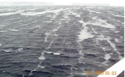
(16) Chapter 1: Introduction. 1.1 The Southern Ocean ice cover The seasonal variability of the sea ice cover in the Southern Ocean is one of the most climatically important features of the southern hemisphere. The area of the planet's surface involved is enormous: the sea ice extent in the Antarctic varies from a minimum of 4x106 km2 at the end of summer (mostly confined to thick, deformed, ice in the far south-western corner of the Weddell Sea) to a maximum of 19x106 km2 in winter. Yet the processes by which the ice forms, especially in the outer part of the pack, are not well understood and have only been studied in situ since 1986 (Wadhams et al. 1987). Investigations of sea ice have instead tended to concentrate on the more easilyaccessible Arctic, where large-scale ice features allow satellite motion-tracking without recourse to expensive in situ instrumentation, and the persistence of ice throughout the year allows its study in summer, when most cruises to ice covered regions occur.. Young ice at the Antarctic ice edge is, by definition, a far more transient form and one which requires the deployment of in situ instrumentation from cruises during the Austral winter. The ice cover begins to advance northwards from March onwards, when cooling of the ocean surface seaward of the summer ice edge starts to freeze the surface waters. The high turbulence levels of the Southern Ocean do not allow this ice to form the familiar coherent sheet (termed ‘congelation ice’). Ice instead forms as a suspension of unconsolidated crystals, known as frazil or grease ice. These are mixed down into the water by the ocean wind and wave fields, often occurring as linear streaks (Figure 1.1), herded into Langmuir plumes (Dethleff 2005; Kempema and Dethleff 2006) with volume concentration around 20-40% (Martin and Kaufmann 1981; Smedsrud and Skogseth 2006) though values of up to 57% have been observed in the laboratory (Newyear and Martin 1997). The mixing allows the continued exposure of sea surface to the colder air, the maintenance of a high ocean-atmosphere heat flux and consequently a much higher ice production rate than would be achieved under calm conditions.. Early studies of frazil crystal formation rates and processes tended to focus on freshwater cases, since these have direct impact in colder countries, such as blocking the cooling water intakes of Canadian power stations (Osterkamp 1978). There has been a. 2.

(17) Chapter 1: Introduction. resurgence of interest in oceanic frazil formation, however, though this has focussed on production in polynyas (Alam and Curry 1998; Smedsrud and Skogseth 2006), and under ice shelves (Smedsrud and Jenkins 2004). Frazil production in polynyas is parameterised in terms of fetch, a threshold wind speed for frazil formation and the frazil collection depth at the downwind edge of the polynya. These have a strong influence on ice production within the polynya and, consequently, how long the polynya remains open and active, but are not applicable to the wave-induced turbulence of the advancing marginal ice zone (MIZ) considered here.. Figure 1.1: Frazil ice forming in a coastal polynya off Kap Norvegia in the Antarctic. Air temperature was -17°C with a wind speed of 20 m s-1.. In the case of ice shelves, rising, supercooled water forms frazil (termed ‘platelet ice’ in this context) as it flows underneath the ice shelf under buoyancy forcing. Accumulation of this frazil forms ‘marine ice’, which becomes visible as striking dark-green ice when icebergs, calved from the ice shelf, turn over as they melt (Warren et al. 1993).. 3.

(18) Chapter 1: Introduction. Figure 1.2: A ‘green’ iceberg, formed from frazil ice accumulating at depth under an Antarctic ice shelf. This iceberg was photographed in open water north of the Weddell Sea ice edge. Also evident are bands of sediment, presumably scavenged by the rising frazil crystals.. In the MIZ, the frazil suspension gradually consolidates into small cakes – known as ‘pancake ice’ – by the agglomeration of the crystals, driven by the absorption of shortwave energy by the frazil slick and augmented by the cyclic compression and rarefaction under the influence of passing troughs and peaks (respectively) of longer waves. Agglomeration is assumed to occur both from below and laterally as the buoyant crystals rise to the surface, with the consolidation being driven by the temperature gradient to the cold atmosphere (Shen et al. 2001). A frazil slick has never been observed to be deeper than the pancakes embedded within it, though upwardlooking sonars have observed the presence of deep scattering layers in coastal polynyas (Drucker et al. 2003), suggesting this does occur in the presence of wind-induced mixing. The frazil crystals are sintered together at their point of contact, minimising their surface free energy (Martin 1981). This overcomes their noted reluctance to stick. 4.

(19) Chapter 1: Introduction. together, caused by an enveloping layer of brine (Hanley and Tsang 1984), contrasting with the behaviour of freshwater frazil crystals which rapidly form relatively strong aggregations or “flocs” (Martin 1981). Using shadowgraph techniques, brine has been observed streaming from crystals both as they ascend under buoyancy forcing after their initial formation, and from an established frazil layer (Ushio and Wakatsuchi 1993). This brine drainage continues as the pancakes age, with relatively open structure allowing very rapid salinity reduction compared to the congelation ice equivalent.. The pancakes are initially only a few centimetres in diameter and are known as ‘shuga’ (Figure 1.3) in their earliest agglomerations (Armstrong et al. 1973) or ‘dollar pancakes’ (Wadhams and Wilkinson 1999) as the disc form becomes more pronounced. The size of the pancakes is controlled by the dominant wavelength (λ) present. Tank experiments. Figure 1.3: Shuga; the first stage in the agglomeration of frazil crystals in the pancake cycle. The photograph was taken looking straight down from the ship’s aft deck, with the individual agglomerations around 5 cm diameter.. 5.

(20) Chapter 1: Introduction. suggest that pancakes are approximately 0.01λ in diameter (Leonard et al. 1998b) and a theoretical framework which broadly matched this result was developed by Shen et al. (2001). Lateral growth occurs by the freezing on of frazil crystals from the surrounding slush and by the agglomeration of other mature pancakes. Frazil is piled onto the edges of the pancakes as they come together, forming slushy ridges up to several centimetres high. Vertical thickening can also occur by rafting one pancake onto another, through either large-scale or local compression.. Figure 1.4: Mature pancake ice, displaying multiple rafting and agglomeration of smaller pancakes. Raised rims are particularly evident in this view. The stick towards the middle of the photograph is one metre long.. The wavelength/pancake size relation continues to evolve as the shortest waves are damped in their progress across the ice cover and the dominant wavelength increases, until pancakes of more than 5 m diameter and 50 cm thickness are observed. Only at a. 6.

(21) Chapter 1: Introduction. considerable distance from the ice edge – up to 270 km (Wadhams et al. 1987) - is the ocean swell damped enough to allow the pancakes to freeze together to form a continuous ice sheet, termed “consolidated pancake ice”. This then thickens, by the usual processes of congelation ice growth on its underside and snowfall on its upper surface, to form the familiar pack ice.. The pancake cycle thus exerts a dominant influence on Antarctic ice types (Weeks 1998) and textural investigations of ice in the central Weddell Sea have revealed that pancake ice growth is the dominant mechanism for pack ice formation in this area (Clarke and Ackley 1984; Gow et al. 1987; Lange et al. 1989; Lange and Eicken 1991).. The importance of pancake ice formation lies in the fact that an ice cover of reasonable thickness can establish itself despite a high oceanic heat flux (Squire 1998). The ice growth is thought to occur at near the open water rate (Wadhams et al. 1987), though quantitative estimates of growth rates during pancake formation are currently entirely lacking. Once the cover cements together to become continuous, growth drops rapidly to the low levels consistent with a c.50 cm thick ice cover. This subsequent rate is in fact almost zero in the Weddell Sea, since the oceanic heat flux then almost balances the loss by conduction through the ice (Gordon and Huber 1990). Wadhams et al. (1987) estimated that only 4 cm of further ice growth took place after the pancake ice cover consolidated.. This thesis aims to increase our understanding of these early stages of ice growth, using data from a drifting buoy array, deployed into the Weddell Sea pancake ice by the author in April 2000. The next sections detail these buoy deployments and set out the scope of the thesis.. 1.2 Data sources The dearth of knowledge about pancake ice has stemmed largely from the fact that no in situ instrumentation had been deployed into a pancake zone, other than three positiononly buoys into the Odden region of the Greenland Sea (Wilkinson 2005). Field. 7.

(22) Chapter 1: Introduction. experiments in the MIZ instead focussed on instrumenting relatively large floes before recovery a short time afterwards, most notably as part of the MIZEX (Bering Sea, February 1983; Fram Strait, July 1983; Greenland Sea, June-July 1984) and LIMEX (Newfoundland, March 1987 & March 1989) experiments (Wadhams and Squire 1986; Wadhams et al. 1988; Liu et al. 1992). The only previous experimental data covering the growth of pancake ice and its transition to pack ice came from tank experiments (Shen and Ackley 1995; Leonard et al. 1998a; Onstott et al. 1998). These suffered from something of a scaling problem, since frazil crystals are ‘life-sized’ while other parameters are not. Limitations of satellite systems (i.e. the Argos system) made the satellite telemetry of large amounts of data impossible and locations were infrequently (three-hourly) and inaccurately (c.350 m accuracy) assessed (Geiger et al. 1998).. The author therefore proposed and was funded (Natural Environment Research Council Grant No. GR3/12952) to design and deploy an array of six drifting buoys into the advancing ice edge region of the Weddell Sea, during the ANT-17/3 cruise of the Alfred Wegener Institute’s research vessel Polarstern (Doble et al. 2001). The buoys were designed to survive harsh impact conditions while mimicking the response of the pancakes to wind and waves. They were also designed to freeze into the ice once the pancakes consolidated, with a tapered hull shape allowing the buoys to be squeezed up and out of the ice should significant convergence be encountered. Figure 1.5 shows one of buoys afloat, shortly after deployment down the ship’s stern ramp.. The buoys were comprehensively instrumented, measuring their GPS position every twenty minutes, meteorological parameters (wind speed and direction, air temperature) every hour and a vertical wave spectrum every three hours. Data were transmitted over the Orbcomm low-Earth orbit (LEO) satellite system (Meldrum et al. 2000) to cope with the relatively large data volumes generated. A standard MetOcean surface velocity profiling barometer (SVPB) buoy was incorporated in the design, as a backup to the untried and hastily-assembled Orbcomm system. The SVPB independently transmitted air pressure data and Argos positions to the Global Telecommunications System (GTS) for use by operational weather forecasting models (Tenhunan et al. 2007).. 8.

(23) Chapter 1: Introduction. Figure 1.5: One of the six ‘pancake buoys’, afloat in the Weddell Sea. The orange sphere in the middle of the buoy is the self-contained MetOcean SVPB Argos buoy.. The buoys were deployed in a ‘five dice’ pattern; with one buoy at each corner of a c.100 km square and the fifth unit in the centre. The array was positioned near the centre of the Weddell Gyre (Kottmeier et al. 1997), in order to minimise advection and hence maximise residence time in the ice. An additional unit was deployed c.300 km further to the west, to verify that the motion of the main array was representative of the ice edge as a whole. This is subsequently referred to as the “long-scale buoy”. This arrangement was found to provide the best compromise between cost and dynamical information in previous MIZ campaigns (e.g. the MIZEX experiments in the Arctic, 1983-9).. Deployment positions are shown in Figure 1.6, which also shows the ice concentration at their deployment, from passive microwave (SSM/I) satellite data. An algorithm developed by the Danish Technical University (DTU) was used to process the raw SSM/I data as this had been optimised for young, wet ice, such as pancakes (Pedersen. 9.

(24) Chapter 1: Introduction. and Coon 2004). The numbers show the nomenclature employed for the buoys, which are numbered sequentially (DML4 – DML9) according to their electronics package.. Figure 1.6: Buoy deployments (blue dots) at the ice edge of the Weddell Sea, shown superimposed on SSM/I ice concentration (colour scale in percent) for 20 April 2000. Low concentration areas in the far west and southeast are the algorithm’s response to glacial ice shelves, not indicated by the grey land mask. The ship track is shown in white. The numbers indicate the buoy IDs referred to in the text.. The buoys proved to be very robust, with all six units surviving the critical pancake consolidation phase. The resulting dataset is unique, since no-one had previously placed buoys so close to the advancing ice edge and watched consolidation proceed.. Further data are provided by the European Centre for Medium-range Weather Forecasting (ECMWF), in the form of six-hourly analyses of meteorological parameters obtained via the British Atmospheric Data Centre (BADC). The author also took part in the collaborative European INTERICE project at the Hamburg large-scale ice tank facility (Thomas and Wilkinson 2001), which provided verification of processes inferred from the Weddell field experiment.. 10.

(25) Chapter 1: Introduction. 1.3 Scientific Aims This thesis aims to produce a better understanding and parameterisation of the pancake ice cover in terms of ocean-ice-atmosphere heat fluxes, momentum transfer and ice growth. Pancake ice is a difficult medium to study given its small size and rapidly changing aggregations, and the dynamic environment essential for its formation and survival. Much therefore remains to be done in understanding its formation and response to wind and wave forcing. We cannot hope to portray the overall ice cover accurately without knowing the evolution of ocean-atmosphere heat flux, ice formation (and concomitant salt injection to the upper ocean), drift and deformation across this vast area of the Antarctic. Specific questions which the thesis seeks to answer are: •. What are the characteristics of the unconsolidated ice motion (both absolute and relative) at time scales which are newly-resolvable by these GPS data (20 minute intervals), but not seen in Argos positions (three hour intervals)? How do the airice momentum transfer coefficients change as the ice consolidates and ages? What are representative values of wind factor and turning angle for Antarctic pancake ice?. •. What is the rate of ice production during pancake formation? How does it compare to the two limiting cases of congelation ice growth (slowest) and frazil ice production at a free surface (fastest)? What are the processes involved in building a pancake from the surrounding frazil slush?. •. What are the implications of any differential motion (convergence/divergence cycles) for ocean-atmosphere heat flux and hence ice production within the ice cover? Do current models accurately represent these values?. 1.4 Thesis structure The study consists of three data chapters, preceded by an introductory chapter and followed by a discussion chapter which brings the results together into a coherent whole. The output of one chapter is used in the next, moving towards a better parameterisation of the young ice cover in terms of ocean-ice-atmosphere heat and momentum fluxes. The data chapters of the thesis are:. 11.

(26) Chapter 1: Introduction. Chapter Two (Dynamics) presents a detailed analysis of the drifting buoy data, with particular emphasis on the additional information provided by the high resolution (temporal and spatial) of the buoy locations. The onset of consolidation (when pancakes freeze together to form a continuous pack) is established and the dynamical contrast between the two regimes examined, particularly with respect to the momentum transfer and differential kinematic parameters (DKPs). The analysis is used as input to later chapters.. Chapter Three (Thermodynamics) describes a new mechanism for the growth of pancake ice and uses modelling to support the hypothesis. In doing so, an attempt is made to quantitatively describe the growth rate of pancakes by both ‘classical’ and novel mechanisms, in an advance to the oft-stated but never qualified “fast”. The air-ice momentum transfer parameters calculated in the previous chapter are used to drive the kinematic portion of a thermodynamic-kinematic model, which tracks the movement of the ice back from the observation time to its formation and extracts the appropriate forcing from ECMWF and in situ meteorological data as it goes. The thermodynamic model then uses this forcing to grow ice forwards in time, using both congelation and free-surface frazil parameterisations. The observed pancake thicknesses (corrected for area and volume concentration) are then compared to these two limiting cases to derive a comparative rate for ice production.. Chapter Four (Growth and motion) combines the growth model and rates, developed in the Chapter 3, with the DKPs developed in Chapter 2 to examine the implications of differential motion for ice production. The divergence-convergence cycles undergone by an ice cover are often termed the “ice accordion” since the motion enhances ice production by exposing open water during the divergent events (allowing rapid ice growth) and redistributing ice (building ice thickness) during convergence. We postulate that any motion at the short time scales measured by the buoys has a significant impact on the magnitude of the ocean-atmosphere heat flux within the ice cover and the volume of ice produced as a result. To elucidate this effect, the thermodynamic growth model is combined with a model for the redistribution of ice thickness by deformation (rafting and ridging), driven by the previously-calculated. 12.

(27) Chapter 1: Introduction. DKPs. Ice is grown applying the growth rate versus thickness relations determined in the previous chapter. The combined model is driven with both the 20-minute forcing measured by the buoys, and with a low-pass filtered timeseries more representative of previous, Argos-based, instruments.. A final chapter then discusses the results and conclusions of the thesis, and suggests further work to deal with the remaining questions.. 13.

(28) Chapter 2: Dynamics. CHAPTER 2: DYNAMICS. The aim of this chapter is to determine the particular dynamic characteristics of pancake ice, contrast them with the more familiar pack-ice and examine whether high-frequency motion plays a significant role.. 14.

(29) Chapter 2: Dynamics. 2.1 Introduction The main innovation of the Weddell Sea buoys was to measure accurate GPS positions at relatively short time intervals. The unconstrained nature of the pancake ice suggested that motions at higher frequencies than traditional Argos measurements could resolve may be significant and that short time-scale alternations of convergence and divergence might have important implications for overall ice production rates through exposure of new sea surface. Studies by Leppäranta and Hibler (1987), for instance, suggested that more than 25% of the energy of the strain rate invariants in sea ice may occur at periods between 30 minutes and three hours. Though the 1983 Marginal Ice Zone Experiment (MIZEX ’83) measured the positions of ice floes at three-minute intervals (using radar transponders), such high-frequency measurements have never been performed in the highly mobile pancake zone, to the author’s knowledge.. The GPS positions, apart from being more frequent, are also considerably more accurate, allowing an improved representation of the buoys’ (hence the ice’s) drift. The location qualities of the two systems are demonstrated by Figure 2.1, which compares a section of drift track: GPS locations clearly show loops and meanders in the track, which are masked by the poor quality of the Argos fixes.. DML4 GPS and Argos fix comparison GPS Argos. -68.94. -68.96. -68.98. -69. -69.02. -69.04. -69.06. -69.08. -69.1. -69.12 -34.35. -34.3. -34.25. -34.2. -34.15. 15. -34.1. -34.05. Figure 2.1: A section of drift track, showing the greatly increased quality of locations afforded by the 20minute interval GPS locations (red), over the more traditional Argos system (blue)..

(30) Chapter 2: Dynamics. The buoys were originally deployed at a slight embayment in the ice edge - as seen in Figure 1.6 - and it was expected that the boundary between pancake and pack ice (the consolidation boundary) would advance smoothly through the buoy array as the season progressed. In fact, the ice advanced northwards on either side of the array while remaining essentially stationary at the buoys’ longitude, leaving the buoys in a deep embayment. This bay then froze rapidly, with the 60% ice concentration contour advancing more than three degrees of latitude between April 30th and May 4th, leaving the buoys far from open water and the influence of wave action. The progress of the 60% ice concentration contour is shown in Figure 2.2, colour-coded by day-of-year:. Figure 2.2: Position of the 60% SSM/I-derived ice concentration contour, showing the pinching-out and rapid freezing of the embayment into which the buoys were deployed. Colour scale shows day-of-year. The buoys were deployed between Days 108 and 110.. This extensive freezing was driven by both the removal of the wave field’s mechanical constraint and a significant drop in air temperature. Both aspects resulted from a lowpressure system passing over the embayment, with its associated winds switching from. 16.

(31) Chapter 2: Dynamics. relatively warm (-2°C) on-ice northerlies, to cold (-17°C) off-ice southerlies, with reduced fetch and thus reduced ability to raise a significant wave field.. Though unforeseen, this rapid transition from unconsolidated pancakes to a situation where the buoys are embedded deep within the consolidated pack ice is ideal for comparing the dynamical behaviour across a sharp consolidation boundary, and this is done in the following sections. The timing of consolidation at each buoy site is examined in the next section.. 2.2 Detection of consolidation The most reliable indication of the onset of consolidation is the wave spectra measured by the buoys, since the passage of waves is the physical phenomenon which prevents the freezing together of the pancakes and hence maintains the unconsolidated cover. Figure 2.3 shows the significant waveheight, Hs, and mean period T1 for three of the buoys, located at the outer, middle and inner pancake zones. Parameters are calculated from spectral moments transmitted by the buoys:. H s = 4.m10 / 2 T1 = m0 / m1. (Eq. 2.1) (Eq. 2.2). where mn is the nth spectral moment, calculated using the relation: N. n mn = ∑ f centre (i ).Δf . p (i ). (Eq. 2.3). i =1. where p(i) is the power spectral density (PSD) vector, Δf is the frequency interval of the calculated PSD and fcentre is the centre frequency of a given interval. Though rather an abstract concept, spectral moments allow the calculation of parameters without requiring the subjective choice of thresholds, as would be necessary for time domain approaches.. 17.

(32) Chapter 2: Dynamics. Figure 2.3: Significant waveheight and mean period for three buoys in the array, showing the sharp reduction following consolidation on May 3rd.. Waveheights decreased with distance from the ice edge, with the outer buoys measuring a peak value of around 3 m and inner buoys showing little vertical motion at any time. Wave motion effectively ceased for all buoys by May 3rd 2000. Mean wave periods evolved from low initial values (7 – 8 seconds) at the outer buoys, to a consolidated value of more than 20 seconds by May 3rd. Inner buoys displayed a period close to 20 seconds throughout.. Determination of the exact time of consolidation was made with reference to the full spectra for each buoy, such as that shown in Figure 2.4, and the buoy heading (its orientation with respect to magnetic north), which also showed considerable contrast across the boundary: the axisymmetric buoys were free to rotate in pancakes, but remained fixed once the ice sheet consolidated.. 18.

(33) Chapter 2: Dynamics. Dates of consolidation, and hence the duration of the pancake phase at each buoy, are shown in Table 2.1.. Figure 2.4: The evolution of power spectral density (PSD), displayed here as a contour plot of log10(PSD) in units of m2s. The sharp drop in power at the consolidation boundary (May 3rd) is clearly shown.. Table 2.1: Buoy deployment details. Columns give the position of the buoy within the ice edge (i.e. outer is furthest north), together with the dates of deployment, consolidation (transition from pancake to pack ice) and last transmission over the two satellite systems. All dates refer to the year 2000.. Buoy ID. Argos ID. WMO ID. Position. Deployed. Consol/d. Last Orbcomm. DML4. 16187. 71583. DML9. 19080. DML5. Inner. 19 Apr. 20 Apr. 15 May. 15 May. 71581. Inner. 17 Apr. 18 Apr. 3 Aug. 3 Nov. 19075. 71511. Centre. 18 Apr. 29 Apr. 13 Oct. 24 Oct. DML7. 19079. 71513. Outer. 18 Apr. 2 May. 30 May. 14 Sept. DML8. 19076. 71512. Outer. 17 Apr. 3 May. 14 Jul. 20 Dec. DML6. 19081. 71582. Long-scale. 20 Apr. 30 Apr. 13 Jul. 15 Sept. 19. Last Argos.

(34) Chapter 2: Dynamics. 2.3 GPS issues. Before comparing drift behaviour across the consolidation boundary, it should be noted that the consolidation of the outer buoys on May 2nd and 3rd coincided almost exactly with the ending of intentional degradation of GPS accuracy available to civilian users. This degradation – termed selective availability, or SA – was removed at 0430Z on May 2nd 2000. It must be ensured that the dynamical differences in the behaviour of pancake and pack ice, derived from these GPS positions, are free from the effects of the varying positional accuracy between SA and non-SA eras.. To this end, data from a GPS base station installed at the German Neumayer station (70°39’S, 8°15’W) prior to the deployments is examined. The base station was installed at the beginning of the cruise to enable differential post-processing correction of the buoy positions and achieve an SA-era position accuracy of around 10 m.. The statistical distribution of position errors before and after the SA transition was examined. The situation is slightly complicated by the fact that Neumayer is moving slowly northwards as its ice shelf advances towards the sea. The position error was calculated from both the mean and median position during Week 18 (the consolidation week). Little difference in statistical descriptors was found between the two methods, and the mean was used for further work since this includes all data and is a more statistically valid approach. Identical length data (3082 points) were used before and after the SA transition.. The difference in errors either side of the transition is striking. Position data had a median of 18.0 m and variance 143.9 m during the SA era. In the post-SA era, median and variance were 2.8 m and 5.2 m respectively. Both ‘before’ and ‘after’ data fail the Kolmogorov-Smirnov test for normality, but fitted gamma distributions well. No statistically-significant difference (using the Mann-Whitney rank sum test) was found between modelled distributions and the actual data, to a high confidence level (P=0.729 and 0.745 respectively). Modelled and real data are shown in Figure 2.5.. 20.

(35) Chapter 2: Dynamics. Neumayer base station, wk18 SOW>1.85x105s 0.045 Data Gamma: a=2.7837, b=7.2424. 0.04. Figure 2.5: Modelled and real data compared for SA (top) and post-SA era (bottom) position errors for the Neumayer station DGPS base station. The gamma distributions can be seen to fit the data well.. 0.035. Probability. 0.03 0.025 0.02 0.015 0.01 0.005 0. 0. 10. 20. 30 40 50 Position error, m. 60. 70. 80. Neumayer base station, wk18 SOW>1.85x105s 0.35 Data Gamma: a=2.7552, b=1.1444 0.3. Probability. 0.25. 0.2. 0.15. 0.1. 0.05. 0 0. 5. 10. 15. Position error, m. Velocity errors were examined and also fitted gamma distributions to a high degree (P=0.902 and 0.964). Median error speeds were 0.89 cm s-1 and 0.13 cm s-1, with variances of 4.5 cm s-1 and 0.03 cm s-1 for SA and post-SA eras respectively. These errors are smaller than would be obtained from applying the mean position error for each period, i.e. we might expect the velocity errors to be of the order of:. uerr = verr = 2. xerr Δt. (Eq. 2.4). where uerr, verr are the component velocity errors, xerr is the mean position error and Δt is the timestep (Geiger et al. 1998). This gives expected scalar velocity errors of 3.4 cm s-1 and 0.5 cm s-1 for SA and post-SA eras respectively, whereas we achieve. 21.

(36) Chapter 2: Dynamics. approximately one third of these figures. The magnitude of these speed errors (c.f. an RMS drift speed around 25 cm s-1) shows the value of GPS fixes over Argos positions: Argos velocity errors are typically around 5 cm s-1, with a three hour fix interval (Geiger et al. 1998).. Modelled errors were used to degrade the post-SA buoy positions, to achieve the same error distribution as the SA-era fixes and ensure that any dynamical differences are due to physical, rather than instrumental, changes. A series of random numbers fitting the SA model were generated and imposed at a random angle on the post-SA positions. The resulting distribution is similar to the SA-era data (P=0.790 from Mann-Whitney). All further analysis was performed on this “error normalised” position data.. An additional complication arises, since the buoys experienced differing rates of GPS position loss (drop-out) during their lifetimes. A GPS almanac bug in the buoy control code resulted in an increasing rate of drop-outs after the initial deployment. Remotely rebooting the units over the two-way Orbcomm satellite link cured the problem, but marked differences remain between buoys and with time. Daily valid fix proportions (of the required 72 per day) are shown in Figure 2.6, which displays the steady decline during the first 25 days of deployment.. Daily successful GPS fixes 1 0.9 0.8. Fix rate. 0.7 0.6 0.5 0.4 DML4 DML5 DML7 DML8 DML9. 0.3 0.2 0.1 105. 110. 115. 120 125 Julian Day. 130. 135. 140. Figure 2.6: The proportion of daily valid fixes achieved by each buoy in the array, prior to being remotely-rebooted to cure the problem.. 22.

(37) Chapter 2: Dynamics. These missing fixes tend to reduce the high-frequency power present in a buoy’s drift record, reinforcing the expected decline in HF power caused by increasing rectification of the ice movement as the pack consolidates. The effect will be minimised for DML7 and DML9, however, since these retain a similar fix rate throughout the period of interest. Missing fixes were interpolated to the standard 20-minute interval using a cubic spline technique. The interpolation is demonstrated in Figure 2.7, which shows a large gap in DML5’s record (this buoy had the most numerous drop-outs). -68.7. -68.75. -68.8. -68.85. -68.9. -68.95 -33.5. -33.4. -33.3. -33.2. -33.1. -33. -32.9. -32.8. -32.7. Figure 2.7: Cubic spline interpolation of DML5’s drift track. Actual position fixes are indicated by crosses, with the cubic spline interpolated portion of the track shown in red. The spline follows the curvature of the track at either end of the gap, filling it in a more realistic manner than simple linear interpolation (straight blue line).. Drift analysis. Analysis of the buoy drift data is split into three sections: •. Drift of the individual buoys. •. Transfer functions between buoy drift and wind forcing. •. Relative motion of the buoys in the array. 23.

(38) Chapter 2: Dynamics. Each is considered first in the time domain, then in the frequency domain. Since the drift parameters were expected to vary as the ice cover evolved, calculations were generally done using a running window, set to 10 days duration, moving forwards at one-day intervals. The window length was chosen to be similar to the duration of the pancake phase of the outer buoys, while providing sufficient samples within the window to allow robust calculations.. 2.4 Drift velocities. 2.4.1 Time Domain The buoys had initial scalar drift speeds of between 22 and 35 cm s-1. The scalar speed of each buoy was largely determined by its v-component (north-south, approximately perpendicular to the ice edge). The drift speed of all buoys fell gradually during the deployment, reaching a minimum of 18 cm s-1 by August (mid-winter) shown in Figure 2.8. The trend was not reflected in the 10-day average winds (ECMWF, 10 m level), which remained around 4 m s-1 throughout.. During the initial period, the outer buoys had significantly higher drift speeds (29 – 35 cm s-1) than the inner buoys (23 cm s-1), with the central buoy having an intermediate response (29 cm s-1). The disparity was not reflected in the local wind forcing, as measured by the buoys’ anemometers. The behaviour was a robust character of the motion, since very similar trends were observed with varying lengths of the running window. Scalar variance – defined as the root-sum-square of the component velocity variances (Kottmeier et al. 1997) – was low, at around 2 cm s-1. Drift speeds for all remaining buoys became very similar past Day 160 once the array was embedded in the pack ice far from the open ocean. Drift speeds continued to fall past Day 180, mostly explained by the reduction in wind speed experienced by the array, before picking up once more as the only surviving buoy began to be influenced by the increasing wind speeds above the Antarctic Circumpolar Current (ACC) at the northern limit of the pack ice.. 24.

(39) Chapter 2: Dynamics. Figure 2.8: Scalar RMS drift speeds for all buoys, for the entire duration of their deployments, calculated with a running 10 day window advancing in one day steps. Also plotted is the scalar wind speed measured by the central buoy (DML5), scaled by 0.1 to plot on the same axes.. 2.4.2 Frequency domain The relatively low number of samples during the unconsolidated phase (less than 1118) makes producing a useful power spectral density something of a challenge. The following methods were compared: •. Simple periodogram, 1024-point FFT (zero padded when shorter) with various windows applied. The Kaiser window, with β set to 7 to ensure the window drops to zero at record ends, provided the best compromise between spectral resolution and variance. •. Welch averaged/overlapped segments, using (a) 2x512-point segments, (b) 4x256-point segments, overlapped by 50% of their width and windowed with boxcar, Hamming, Kaiser and Parzen windows. This is a similar method to that. 25.

(40) Chapter 2: Dynamics. used in the on-board wave spectrum algorithm of the buoys themselves, as it gives the smallest possible variance per data point •. Thompson’s multi-taper method, with various time-bandwidth parameters. This gave inferior results in the high-frequency part of the spectrum. The two-segment, overlapped Welch method with Hamming window gave the best results and this was used in all further FFTs. Example v-component spectra for DML7 (outer MIZ) and DML4 (inner MIZ) are shown in Figure 2.9, together with those for the in situ (1 m ASL) windspeed measured at DML7. Spectra are plotted for the preconsolidation period of DML7 and for an equivalent period (11 days) postconsolidation.. Figure 2.9: v-component drift spectra for outer (DML7) and inner (DML4) ice edge buoys. Only one spectrum is plotted for the inner buoy, since the post-May 2nd spectrum is very similar to that shown and is therefore omitted for clarity. Also shown are spectra for the scalar in situ windspeed measured at DML7.. 26.

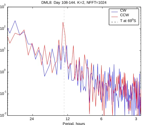
(41) Chapter 2: Dynamics. All spectra show increasing spectral power towards the low-frequency end of the spectrum. This ‘red noise’ behaviour is characteristic of many geophysical parameters and persists here when the mean (DC component) of the drift is removed, as done here.. Considerable contrast is evident between pre- and post-consolidation spectra for the outer buoy, with higher power at all frequencies and an order of magnitude increase at high frequencies during the pancake phase. The increased contribution of motion at timescales shorter than six hours is clearly shown by the elevated power in DML7’s preconsolidation spectrum. This energy is not present post-consolidation. The scalar in situ wind spectra show no such contrast. The inner buoy displays little change in its spectra between the two periods, and the post-May-2nd spectrum is omitted for clarity. Power in both phases is similar to that shown by DML7’s post-consolidation spectrum.. The significant peak in the buoys’ post-consolidation drift at around 12 hours was investigated using rotary spectra (Emery and Thomson 1998) to determine whether its origin was tidal or inertial: inertial motions only appear in the counter-clockwise (CCW) component for the Southern Hemisphere, while tidal cycles appear in both clockwise (CW) and CCW spectra. Figure 2.10 shows the peak in the CCW spectrum only, indicating the inertial nature of the oscillation. The inertial influence is expected, since the array was deployed in an area of very little tidal influence (Padman and Kottmeier 2000). Also marked on Figure 2.10 is the inertial period at the buoy’s latitude, given by:. T = π / ω sin φ = 12.85 hours. (Eq. 2.5). Where φ is the latitude and ω is the angular velocity of the Earth, 7.272×10-5 rads s-1. The dominance of the inertial peak suggests that the pack ice is essentially in free-drift behaviour throughout, since relatively compact ice fields tend to damp inertial motion due to phase mismatches between nearby interacting inertial cycles (McPhee 1980).. 27.

(42) Chapter 2: Dynamics. DML8: Day 108-144. K=2, NFFT=1024. 3. 10. CW CCW T at 69oS. 2. 10. 1. 10. 0. 10. -1. 10. -2. 10. 24. 12 Period, hours. 6. 3. Figure 2.10: Rotary spectra for DML8, showing the inertial peak in the CCW spectrum only. The inertial period of 12.85 hours is indicated by the dotted line. (Matlab code for rotary spectra courtesy of Timo Vihma, FIMR).. The effect of missing fixes on the HF spectra, mentioned in the previous section, was investigated by imposing an artificial drop-out rate on otherwise complete data. Even inflicting the maximum loss rate seen (32%) had very little effect on the resulting spectrum, and any differences in this portion of the spectrum result from physical differences alone. The time evolution of the spectra was examined with reference to the spectral slope (α). Slope was calculated from the spectrum between 3-hour and 12-hour periods, corresponding to the largely linear (in log-log space) portion of the spectrum. Spectral slope is defined as:. S = ω −α. (Eq. 2.6). where S is power spectral density and ω is the angular frequency. Results are displayed in Figure 2.11, for the u-component of motion; v-component results are similar.. 28.

(43) Chapter 2: Dynamics. Spectral slopes for the various buoys largely overlay, showing a trend towards increasing values – i.e. a reduction in HF motion – until Day 190 (mid July), with a similar gradient decrease (increase in HF motion) thereafter. The decrease after Day 190 suggests that the pack ice is becoming less constrained after this date, consistent with its generally divergent nature towards the maximum ice extent. Values are lower during the pancake phase than generally seen in the literature (e.g. 3, Leppäranta 2005), consistent with the increased influence of HF motion. They compare with typical values of 5/3 for oceanic velocity spectra at centimetric scales and 2 at eddy scales. The slope for the outer buoys therefore suggests that the ice cover is responding to the oceanic velocities almost without modification (value close to 2).. 3.5 DML4 DML5 DML7 DML8 DML9. Spectral slope. 3. 2.5. 2. 1.5 100. 120. 140. 160. 180 200 Julian Day. 220. 240. 260. 280. Figure 2.11: Spectral slope with time for the full duration of the buoy deployments.. Variations in integrated power at high- and low-frequencies over time were also studied, since changes in the spectral slope give no information on the magnitude of power at any frequency, only its variation over the chosen spectrum. The division between LF and HF regimes was set at 15 hours period, to include the inertial component, and was also investigated at 4 hours cutoff. Results are shown in Figure 2.12 for a 15 hour. 29.

(44) Chapter 2: Dynamics. cutoff. Both cutoff values showed a similar trend, with HF power dropping exponentially (linearly on a log scale) until Day 200 and then increasing thereafter. Characteristics for all buoys again largely overlay, mirroring the character of the α curve. The HF power and α, which both depend on the freedom of movement, correlate at -0.65 < r < -0.88. Power at LF shows a contrasting character, oscillating around a more constant value.. HF <15 hour periods. 8. Integrated PSD/BW. 10. DML4 U DML5 U DML7 U DML8 U DML9 U DML5 V. 7. 10. 6. 10. 5. 10 100. 120. 140. 160. 180. 200. 220. 240. 260. 280. LF >15 hour periods. 10. Integrated PSD/BW. 10. DML4 U DML5 U DML7 U DML8 U DML9 U DML5 V. 9. 10. 8. 10. 100. 120. 140. 160. 180 200 Julian Day 2000. 220. 240. 260. 280. Figure 2.12: Integrated power spectral density per bandwidth, for HF (top) and LF (bottom) periods. HF power shows a cyclical character as constraint is increased then relaxed, while LF power is more constant throughout.. 30.

(45) Chapter 2: Dynamics. The analysis shows that the increase in spectral slope seen previously arises from a very marked reduction in the HF power, which drops by two orders of magnitude between the pancake era and the point of ‘maximum constraint’ (Day 200), while the lower frequency power has a more constant character, oscillating around a mean value and represents the overall advection in the Weddell Gyre. Since the scalar drift speed (Figure 2.8) mirrors the form of the HF curve, it can be concluded that this highfrequency energy contributes significantly to the overall motion of the buoys during their initial deployments.. All parameters suggest a cycle of constraint: As the ice edge advances past the buoys, constraint increases to a maximum in mid-August (Day 200), after which the increasingly divergent nature of the pack ice reduces constraint once more, before the ice finally breaks up at its northern limit in December. The pancake regime does not appear radically different from the pack ice in this aspect of the study, and can be considered a starting point in the cyclical evolution of constraint from the ice’s formation to its break-up.. 2.4.3 Wavelet Analysis The ten-day running window used in the preceding analysis necessarily averages the parameter under study over the window period. It is perhaps interesting to examine whether the unconstrained high-frequency motion is a continuous feature of the pancakes’ motion, or whether it is more periodic, varying as low pressure systems pass the array. Reducing the FFT window length often gives rather arbitrary results, however, as the number of points in the FFT drops to below tractable values. Frequencies are also treated inconsistently in such an analysis, since low frequencies are only represented by a limited number of cycles in each window (reducing frequency localisation - the routine’s ability to discriminate the frequency of a component) while high frequencies have so many cycles in the window that it is difficult to determine where the component begins and ends (time localisation).. Wavelet analysis offers a possible solution to the problem, though it has been criticised for providing ‘pretty pictures’ but little quantitative information, especially with regard. 31.

(46) Chapter 2: Dynamics. to statistical significance. Wavelet routines with significance and confidence testing have been developed (Torrence and Compo 1998), however, and these are used here in an attempt to overcome such objections. Details of the wavelet analysis are given in Appendix A.. Wavelet spectra are shown for the central buoy (DML5, Figure 2.13) for the initial period of interest (to Day 142). The v-component velocity is chosen since it shows the greatest contrast between pancake and pack ice regimes, though the u-component results are similar. The figure demonstrates the additional insight that wavelet analysis can provide: Though the high frequency energy is clearly evident throughout the first half of the timeseries (top graph), it shows considerable power variation in the wavelet spectrum (middle graph), alternating between periods of high energy (yellow) in the 1-6 hour band and even higher energy episodes when the orange colour intrudes into the same band. The periodicity in this variation is of the order of five days, which is approximately the time taken for an atmospheric low-pressure system to pass the array, from the initial, compacting, northerly winds to the final, rarefying, southerlies. Such a conclusion suggests that the highest frequency energy is forced by the wind, but this is not supported by analysis of the in situ wind records themselves, which show no such variation in HF power. The wavelet analysis therefore gives the insight to suggest that variations in the buoys’ HF motion are caused indirectly by the winds – for instance by the wind direction determining the state of compression of the pancake zone, and hence its ability to respond to other, possibly oceanic, forcing.. DML5’s inertial energy appears non-significant (bottom graph) and the inner buoys display even less power in this band, suggesting that these latter buoys undergo more damped motion from the start of their records. Intermittent oscillations are seen in the outer buoy’s plots.. 32.

(47) Scalar speed, ms-1. DML5 0.8 0.6 0.4 0.2 0 110. 115. 120. 125. 130. 135. 140. 115. 120. 125. 130. 135. 140. 1. Period, hours. 3 6 12 24 48. 144 110. Avg. variance. 1 10-15 hr avgd 95% sig 0.5. 0 110. 115. 120. 125 Julian Day. 130. 135. 140. Figure 2.13: Wavelet power spectrum for the central buoy (DML5) around the consolidation boundary. Top graph shows the scalar velocity timeseries. Middle graph shows the wavelet power spectrum, with the cone of influence marked as a yellow line and the 95% confidence contour marked as a thick blue line overlaying a thicker yellow contour. The bottom graph shows the integrated wavelet power across 10-15 hour scales, and is a measure of the total power in the inertial 12 hour peak. The dotted line corresponds to the 95% significance level.. 33.

(48) Chapter 2: Dynamics. 2.5 Momentum transfer coefficients. The preceding analysis demonstrated progressively decreasing scalar drift speeds in the presence of relatively constant wind forcing. These results imply either that the ability of the wind to transfer its momentum to the ice is changing – due, for instance to the ice roughness changing as the ice evolves – or that the influence of other forcing, not related directly to the local wind speed (such as the large-scale wind curl which drives the Weddell Gyre), is varying. The transfer of energy from the atmosphere to the ice and hence to the ocean is important for the modelling community. Parameters must be known accurately in order to model the drift of the ice. The track and hence residence time of a particular piece of ice in the pack determines its rate of formation, thickening (thermodynamically and by deformation) and subsequent melt. Such information allows estimation of heat, salt and momentum fluxes throughout the polar oceans and is crucial to understanding the physical processes operating there. Accordingly, these momentum transfer parameters are investigated in some detail in this section, since values for Antarctic pancake ice are currently entirely unconstrained.. Momentum transfer from surface winds to buoys or ice can be described by a simple linear ratio, known as the wind factor, α, with turning angle, δ, between the wind and the forced object (CCW in the Southern hemisphere). Linear ratios have been shown to approximate the non-linear momentum balance well (McPhee 1980; Thorndike and Colony 1982; Martinson and Wamser 1990; Kottmeier et al. 1992), especially for thin Antarctic ice where the Coriolis term is relatively small. Alternative methods, such as the solution of quadratic drag coefficients, involve assumptions about the roughness lengths of air and water interfaces which are unknown (Thomas 1999).. Wind factor and turning angle were calculated using both the winds measured by the buoys (1 m ASL) and ECMWF 10 m winds, both interpolated to the 20 minute fix interval using a cubic spline. Points with a wind speed value of less than 1 m s-1 were removed, to eliminate sensor freeze-up events (actually quite rare) and light-andvariable conditions. Turning angle was calculated after removing outlying points, which were defined as being those exceeding an absolute angle of more than 120°.. 34.

(49) Chapter 2: Dynamics. In situ wind directions were unfortunately not available from DML6, DML7 and DML8, due to faults in their compasses. Though the headings of other buoys varied through the full 360° during the unconsolidated phase, headings for these three buoys varied through very limited angles (e.g. 280° to 360° for DML7). This is unlikely and points to a fault in these compass units (Honeywell HMR3000) or in their calibrations. It was not possible to perform an in-hull calibration of the compass units, as the buoys were constructed on board the ship in the presence of many hard- and soft-iron influences, but these results indicate that this is essential if reliable directions are to be obtained from future deployments.. The wind direction is calculated (post-transmission) as a combination of the wind sensor direction with respect to an on-board reference and the buoy magnetic heading. Magnetic deviation in the area of the buoys is almost exactly zero, and is ignored. The wind direction information for these three buoys must therefore be completely disregarded, which is unfortunate, since these are the buoys which remained in pancake ice the longest.. ECMWF 10 m winds are generated from pressure analyses at the lowest model level (30 m), estimating the surface roughness length and atmospheric stability (Kottmeier et al. 1997). These 10 m results were then interpolated from the ECMWF 1.125°×1.125° grid to a 0.5°×0.5° grid, using the Kriging technique.. 2.5.1 Buoy and model winds compared The correspondence between modelled (10 m) winds and measured (1 m) winds was examined in terms of their correlation, velocity ratios and turning angles, for scalar speeds and vector components. Results are shown in Table 2.2. Values for the magnitude relation are very consistent and have low standard deviations, though the turning angles have a greater spread.. 35.

(50) Chapter 2: Dynamics. Table 2.2: Magnitude ratio and angle (degrees) between buoy-mounted wind measurements (1 m ASL) and ECMWF 10 m model output, for the whole lifetime of each buoy, expressed as the median and standard deviation (SD). Directions are omitted for buoys with faulty compasses. Calculations for DML5 do not include the period of open water drift at the end of its deployment.. DML. Median. SD. Median. SD. v1/v10. v1/v10. Angle. Angle. 4. 0.60. 0.24. 73. 34. 5. 0.56. 0.29. 53. 53. 6. 0.56. 0.26. 7. 0.57. 0.85. 8. 0.60. 0.37. 9. 0.59. 0.31. 50. 28. Mean. 0.58. 59. The published literature contains few references to winds at this low height, which was dictated by stability requirements in the heavy icing conditions that the buoys were expected to experience. Rare measurements come from ice camps in mature pack ice such as the 0.6 m measurements at Ice Station Weddell (Andreas and Claffey 1995), for which the V0.6:V10 ratio was ~0.25. A minimum height of 4 m is more usual, with quoted transfer coefficients over winter pack ice of 0.53 to 0.55 (with respect to the geostrophic wind), with a turning angle of 7-30o (Vihma et al. 1996; Uotila et al. 2000).. Buoy winds were then rotated by the mean angle calculated above and correlation between buoy and model winds examined, for vector and scalar components. Results are shown in Table 2.3. Coefficients are high for all valid components and scalar speeds. They are similar to those seen in published literature (e.g. Uotila et al. 2000) though sensor heights were typically 4 m there, and give some confidence in the. 36.

No results found