Considerations of Accuracy and Uncertainty with Kriging Surrogate Models in Single Objective Electromagnetic Design Optimization

(1)

Considerations of accuracy and uncertainty with

kriging surrogate models in single-objective

electromagnetic design optimisation

G. Hawe and J. Sykulski

Abstract: The high computational cost of evaluating objective functions in electromagnetic optimum design problems necessitates the use of cost-effective techniques. The paper discusses the use of one popular technique, surrogate modelling, with emphasis placed on the importance of considering both the accuracy of, and uncertainty in, the surrogate model. After a brief review of how such considerations have been made in the single-objective optimisation of electro-magnetic devices, their use with kriging surrogate models is investigated. Traditionally, space-filling experimental designs are used to construct the initial kriging model, with the aim of max-imising the accuracy of the initial surrogate model, from which the optimisation search will start. Utility functions, which balance the predictions made by this model with its uncertainty, are often used to select the next point to be evaluated. In this paper, the performances of several different utility functions are examined, with experimental designs that yield initial kriging models of varying degrees of accuracy. It is found that no advantage is necessarily achieved through a search for optima using utility functions on initial kriging models of higher accuracy, and that a reduction in the total number of objective function evaluations can be achieved if the iterative optimisation search is started earlier with utility functions on kriging models of lower accuracy. The implications for electromagnetic optimum design are discussed.

1 Introduction

Optimisation problems in electromagnetic design are typi-fied by features that present difficulties to most determinis-tic search algorithms, such as the existence of multiple local minima. Genetic algorithms (GAs), on the other hand, with their ability to search more globally, are better suited for exploring complicated objective function landscapes. The high computational cost of evaluating the objective function in such problems, however, means that direct use of a GA is often not feasible or is impractical, owing to their general requirement for a large number of objective function evalu-ations. Additional cost-effective techniques must be used, with the aim to make the GA require fewer evaluations of the objective function. Techniques used include hybrid algorithms [1], GAs that are specially adapted for small population sizes [2] and simplification of the problem by removal of irrelevant design variables [3]. One technique that has recently attracted significant attention, called surro-gate modelling[4], is the focus of this paper.

A surrogate model is a functional relationship between the design variable space of an optimisation problem and the objective function space, which is constructed based on a set of design vectors that have their objective function values known, referred to henceforth as ‘experiments’. Once a surrogate model has been constructed, a GA can

then use it to predict fitness values for unevaluated design vectors, rather than call the true expensive objective func-tion, thus reducing computational costs. Surrogate-assisted optimisation can therefore be viewed as consisting of two separate stages

(i) the construction of the initial surrogate model from a set of experiments (off-line learning)

(ii) the subsequent iterative optimisation search where, during each iteration, predictions from the most recently constructed surrogate model are used to select a design vector for evaluation. Once evaluated, this design vector is then used to construct a more accurate kriging model (on-line learning).

Accuracy and uncertainty considerations play an important role in surrogate-assisted optimisation. In the first stage, the set of experiments is typically chosen with the aim of max-imising the accuracy of the initial surrogate model; this allows predictions made by the model to be used with greater confidence. Uncertainty in the surrogate model is then usually considered during the optimisation search and has an influence on the selection of where to sample next in the design variable space.

This paper includes a brief review of how accuracy and uncertainty considerations have been used with three popular surrogate models (polynomial interpolation, artifi-cial neural networks and kriging) in electromagnetic optimum design. Although reviews of the use of different surrogate models exist in the literature, none focuses on accuracy and uncertainty considerations. The paper also comprises an investigation into how kriging model accuracy depends on features of the experimental design used, and an investigation into how the performance of different utility #The Institution of Engineering and Technology 2007

doi:10.1049/iet-smt:20060035

Paper first received 10th March and in revised form 11th August 2006 G. Hawe is with School of ECS, University of Southampton and Vector Fields Ltd., Kidlington, Oxford, UK

(2)

functions in locating the optimum of several test functions depends upon the accuracy of the kriging model used.

It should be noted that, for the accuracy of a surrogate model to be determined, the true function it is approximat-ing must be known, so that a comparison can be made between the two, and the relevant accuracy statistics can be computed. Real electromagnetic examples are therefore not used in this paper, as the true objective function is almost always unknown. This should not pose any concern anyway, as no problem exists that is truly represen-tative of all electromagnetic optimum design problems; the logic is that there is as much justification in extending con-clusions based on an investigation of three different test functions to real electromagnetic problems, as there is in extending conclusions based on any single electromagnetic design problem to real electromagnetic problems.

2 Use of surrogate model accuracy considerations in electromagnetic design optimisation

2.1 Polynomial approximations

Polynomial approximations are among the most common methods of surrogate model construction. Despite their popularity, however, polynomial approximations suffer in several respects. A minimum number of experiments is required in the experimental design before a polynomial model (of a given order) can be constructed. Also, it is only for this minimum number that the model will actually interpolate the experiments; use of additional points through on-line learning results in an over-determined system of equations, and the resulting polynomial surrogate model will no longer be an interpolating surface, that is the inclusion of additional points into the model does not necess-arily lead to increased model accuracy. Furthermore, if uncertainty considerations are not made during the selection of where to sample next during the optimisation search, so that only the optimum of the surface is added in each iter-ation, not only can the model accuracy decrease, but rapid convergence to a false optimum can occur[6].

In [7], a polynomial surrogate model was used to opti-mise a brushless permanent magnet motor. The accuracy of the model was considered at the two main stages of the optimisation process, namely during the construction of the initial surrogate model from an experimental design, and is the choice of which points to evaluate during an iter-ation of the optimisiter-ation search. The experimental design was constructed so as to minimise the condition number of the matrix [M] that was to be inverted to determine the polynomial coefficients; furthermore, to ensure it was inter-polating (as well as keeping computational cost to a minimum), only the minimum number of points required to construct the polynomial model were used. A dynamic weighting factor was then used, as the optimisation search proceeded, to place more emphasis on the region around the predicted optimum. Then, to ensure that [M] did not become ill-conditioned as the search continued, additional

learning points were evaluated, chosen specifically so as to minimise the condition number of [M]. An analysis of the errors on predicted optima and learning points indicated that the inclusion of learning points was effective in improv-ing the accuracy of the polynomial surrogate model.

2.2 Artificial neural networks

A wide range of different types of ANN exist that can be used to construct surrogate models [8]. One of the most

widely used is the radial basis function ANN [9]. An example of the use of such an ANN in electromagnetic optimum design can be found in[10], where a multiquadra-tic radial basis function was used as a surrogate model in the optimisation of a C-core magnet and a magnetiser. In addition to evaluation of the predicted optimum during on-line learning, design vectors in the most unexplored regions of design space were also evaluated, with the aim of avoidance of local minima. Unexplored regions of design variable space have the highest uncertainty in their values, and so the use of such points in on-line learning facilitated reduction of the uncertainty in the surrogate model as the optimisation search proceeded.

2.3 Kriging

Kriging has recently been recognised as a useful method for surrogate model construction in electromagnetic optimum design[5]. Owing to its statistical nature, useful information can be extracted, giving an indication of model uncertainty. The efficient global optimisation (EGO) algorithm[11]uses such information to build up a utility function, known as the expected improvement, that automatically balances the objective function values predicted by the kriging model with the uncertainty in this prediction. Through optimi-sation of this auxiliary function, model uncertainty is auto-matically considered as the optimum is being searched for. Expected improvement and other utility functions are reviewed in the following section.

A variation of EGO, known as superEGO, has been used to solve two electromagnetic design problems with expens-ive objectexpens-ive functions[12], one with three design variables and one with four. Experimental designs consisting of random points sparsely distributed in design variable space were used to construct the initial kriging surrogate models, and convergence was found to occur within tens of iterations in both cases.

The simultaneous growth in the development of modern experimental designs for computer experiments and that of the use of utility functions with kriging models for optim-isation have motivated this investigation into the relation-ship between the two areas.

3 Kriging model accuracy and experimental design

3.1 Modern experimental designs

All surrogate models are constructed from a set of exper-iments, and it is the purpose of design of experiments[13] to determine the set that will yield the most accurate poss-ible surrogate model. This set will vary according to the nature of the true (unknown) function being modelled, and so generic experimental designs that have desirable properties are often used. Traditional experimental designs are increasingly being replaced by modern experimental designs[14]that have been developed for use with determi-nistic computer experiments. Such designs usually concen-trate on the desirable properties of being uniform and space-filling, although recently the usefulness of such prop-erties has come under scrutiny [15]. Two experimental designs are investigated in this paper

(a) Latin hypercube: a Latin square is a square with each side subdivided, so that there are N rows and Ncolumns.

(3)

dimensions. If each side of the hypercube represents a different design variable,Ndesign vectors can be selected using this design, with the advantage that the number of experiments is independent of the number of design variables.

(b) Hammersley sequence: a Hammersley sequence pro-vides a low-discrepancy set of experiments, in that the points are uniformly distributed in design variable space. For details of the construction of a Hammersley sequence, the reader is referred to[17].

Through consideration of the accuracy of kriging models constructed using these two experimental designs for a simple test function in the following section, two further potentially attractive features of experimental designs for the construction of kriging models have been suggested.

3.2 Potential problem for experimental designs for kriging model construction

Given a set of experiments, a kriging model is defined by a vector u that is found by maximisation of the likelihood function[5]

Nlnðs

2_ð_u_{ÞÞ þ}_ln_ðj_R_ð_u_ÞjÞ

2 ð1Þ

whereNis the number of experiments used to construct the kriging model,s2is the variance as predicted by the kriging model, and Ris the matrix of correlations between the N

experiments, whosei-jth entry is usually formed using the Gaussian correlation function

Rðxi;xjÞ ¼Y n

k¼1

eukjx i kx

j

kjpk _ð₂_Þ

From this, it is clear thatukdetermines how rapidly the

cor-relation is lost in thekth design variable (large values imply-ing rapid loss in correlation), and pk determines the smoothness of the function of the kth design variable (values near 2 denoting smooth functions, values near 0 denoting rough functions). Usually,pk¼2 is used for all

k, and this is the value that will be used for all of the kriging models constructed in this investigation.

The behaviour of the likelihood function determines the value obtained for the vectoru and so determines the behaviour of the kriging model that is constructed. Poor behaviour of the likelihood function is likely to result in a poor value of u being obtained and, consequently, in an inaccurate kriging model. One common example of poor behaviour for this function is monotonicity, as this results in an extremely large value of u being used to construct the kriging model, implying virtually no correlation between any of the design vectors, which is undesirable for most functions.

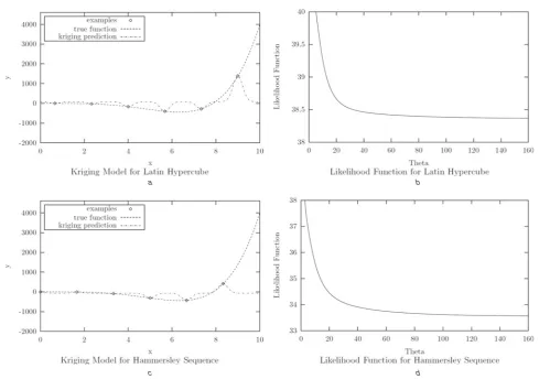
An example of this can be seen inFig. 1, where the Latin hypercube and Hammersley sequence experimental designs have both been used to construct kriging models for the Wilkinson test function[18]

fðxÞ ¼8:9248105x2:18343102x2þ0:998266x3

1:6995x4þ0:2x5 ð3Þ

Each experimental design results in a monotonic likelihood function (note that the negative sign of the likelihood func-tions plotted in the figures has been omitted, so that the like-lihood functions in the figures are now to be minimised), and so, for each kriging model constructed, an extremely

large value of u is used; hence, their inaccuracy. At this point, two potentially attractive features of experimental designs are suggested, and their effect on the behaviour of the likelihood function for constructing kriging models for (3) is examined.

3.3 Potentially attractive features of experimental designs

For ann-dimensional design variable space, the two follow-ing attractive features of experimental designs for the con-struction of kriging models are proposed:

(i) the inclusion of the 2nextreme boundary points of the design variable space; that is, for a problem withndesign variables that vary as xilxixiu, i¼1,. . .,n, the 2n corners of the hypercube that bounds the feasible region in design variable space are included

(ii) for a particular experiment x _{in the experimental} design, the inclusion of n additional experiments a small distance away from x_{, in each of the}_n_orthogonal direc-tions aroundx_.

The first of these features is proposed as kriging models are designed to interpolate points in multidimensional space. Therefore the inclusion of the extreme boundary points in the design variable space in the experimental design means that extrapolation by the kriging model is kept to a minimum. The second of these features is proposed as, because a kriging model interpolates the experiments it is constructed from, the inclusion of such points forces the gradient around the experimentx _{to be highly accurate in} the constructed kriging model.

It should be noted that these features can occur naturally

in some experimental designs (for example, the

Hammersley sequence design will always include one of the boundary points); alternatively, these features can be combined with existing experimental designs, giving a hybrid design that has some of the features of both.

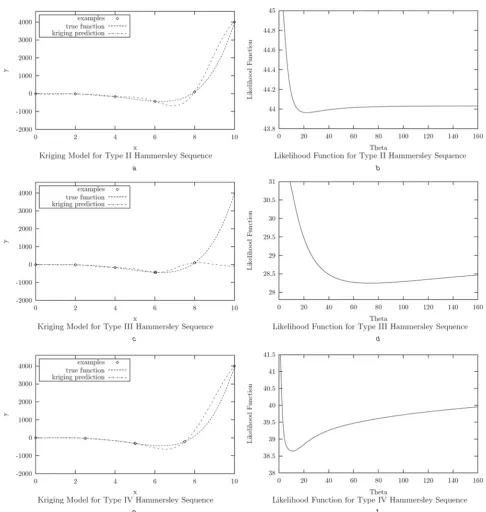
Each of these features will be combined with the Latin hypercube and Hammersley sequence designs, to give two additional variants of each: designs that have boundary points included will be referred to as type II variants, and designs that have the gradient enforced to be correct at a point will be referred to as type III variants (Type I variants will be the experimental design without either feature imposed). In addition, the effect of combining both features simultaneously with an experimental design will be investi-gated; these will be referred to as type IV variants.

The effect of each of these variants on the construction of kriging models for the Wilkinson test function can be seen in Fig. 2. Each variant successfully removes the monotonicity of the likelihood function, resulting in more reasonable values forubeing used to construct the kriging model. Similar results were obtained for the Latin hyper-cube variants. Note that, for fair comparison, the same number of experiments is used in each variant. This means, for example, that a type II Hammersley sequence of size 6 in one dimension actually uses a Hammersley sequence of size 5 (the two boundary points plus the four non-boundary points of a Hammersley sequence of size 5, giving a total of six points).

(4)

3.4 Test functions

Strictly speaking, the true accuracy of a surrogate model can only be determined if the true function, which it is attempt-ing to approximate, is also known and is available for comparison. Almost all electromagnetic optimum design problems are non-analytic, meaning it is impossible to measure the accuracy of any surrogate model constructed. For this reason, the investigation in this paper will be carried out using well-known test functions. In total, three test functions have been selected: one one-dimensional (1D) test function, known as Humps (as used in[19])

fðxÞ ¼6 1

ðx0:3Þ2þ0:01

1

ðx0:9Þ2þ0:04 ð4Þ

one two-dimensional (2D) test function, known as Branin [20]

fðx₁;x₂Þ ¼ ð12x₂þ0:05 sinð4px₂Þ x₁Þ2

þ ðx₂0:5 sinð2px₁ÞÞ2 ð5Þ

and one three-dimensional (3D) test function, known as Hartman3[21]

fðx₁;x₂;x₃Þ ¼ X 3

i¼0

c_iexp X n1

j¼0

A_ijðx_jp_ijÞ2 !

ð6Þ

where the matricesAandpand the vectorcare as defined in [21].

Each of these functions will be evaluated over a mesh of about N¼1000 points (1000 equally spaced points for (4), 3232¼1024 equally spaced points for (5), and

101010¼1000 equally spaced points for (6)). The kriging models are then evaluated over the same meshes for a variety of experimental designs, and compared with the true functions so that their accuracy can be determined.

3.5 Accuracy measures

A variety of methods exist for comparing the surrogate model with the true function to assess its accuracy. Three methods will be used here: the normalised maximum error

NEMAX, the normalised root mean squared error

NRMSE and the Kolmogorov – Smirnov statistic D. NEMAX and NRMSE are defined as

NEMAX¼maxfj_{ffiffiffiffiffiffiffiffiffiffiffiffiffiffiffiffiffiffiffiffiffiffiffiffiffiffiffiffiffiffiffiffiffiffi}yiyîjgi¼1;. . .;N

ð1=NÞPðy_iyÞ2

q ð7Þ

NRMSE¼

ffiffiffiffiffiffiffiffiffiffiffiffiffiffiffiffiffiffiffiffiffiffiffiffiffiffiffiffiffi PN

i¼1ðyiy^iÞ 2 PN

i¼1ðyiÞ2 s

ð8Þ

whereyiis the true value at sitei,y¯iis the value predicted by the kriging model at site i, and y¯ is the true mean of the points at i. Obviously, smaller values of NEMAX and NRMSE indicate greater accuracy. The Kolmogorov – Smirnov statistic D is defined as the maximum distance between the predicted and the true cumulative distribution functions, denotedSN(y) andPN(y), respectively,

D¼ max

1,y,1jSNðyÞ PNðyÞj ð9Þ

with smaller values ofDindicating greater accuracy.

a b

c d

[image:4.595.50.540.22.366.2]

(5)

3.6 Surrogate model accuracy dependence on experimental design

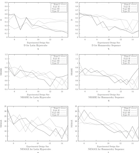
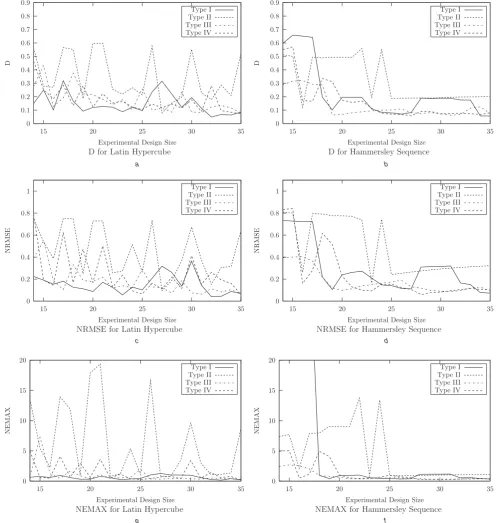
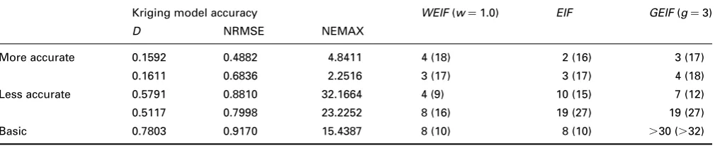
Each of the four variants of the Latin hypercube and the Hammersley sequence was used to construct initial kriging models for each of the three test functions, for varying exper-imental design sizes. The accuracy of the kriging models constructed was then assessed using each of the measures given above. The results are shown inFigs. 3–5.

The results for the 1D Humps problem showed that there is no significant difference in performance between the two main types of experimental design. This is to be expected in one-dimensional problems: for an experimental design size ofn, when the 1D design variable space is divided intonequally sized intervals, the Latin hypercube will place one point at random in each interval, whereas the Hammersley sequence will place one point at the start of each interval. As would

be expected, the trend within each experimental design is that accuracy increases as the experimental design size increases, but this increase is perhaps not as significant as we might expect. For small experimental design sizes, some increase in accuracy resulted from the imposition of the suggested features; however, no general increase in accuracy was found in experimental designs of greater size.

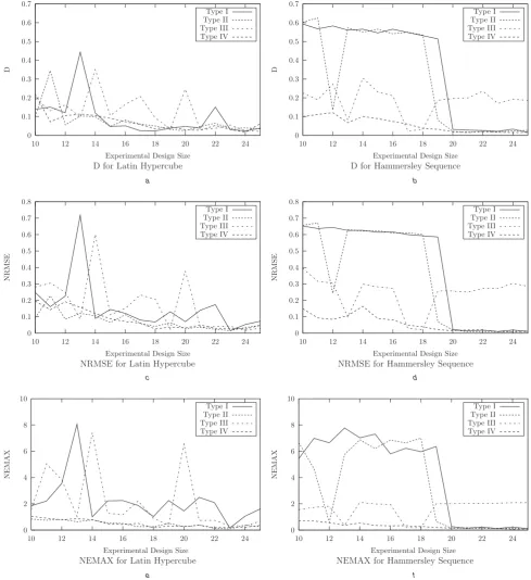
Results for the 2D Branin function showed clearer trends. The simultaneous forcing of the gradient to be correct at a point and inclusion of the boundary points yielded signifi-cant increases in accuracy by all measures for both exper-imental design types, particularly the Hammersley sequence design. The enforcing of a correct gradient at a point gave increases in accuracy when combined alone with the Hammersley sequence design; however, its per-formance, when combined with the Latin hypercube, did not always result in an increase in accuracy.

a b

c d

e f

[image:5.595.56.543.22.535.2]

(6)

Results for the 3D Hartman3 function showed that inclusion of the boundary points in either design in general did not give an increase in accuracy. However, the combination of either or both of the suggested features with the Hammersley sequence design led to an increase in accuracy for smaller design sizes. The forcing of the gra-dient to be correct at a point in the kriging model tended to result in an increase in accuracy, although this gain in accu-racy lessened as the experimental design size grew.

In general, the only feature of experimental designs that con-sistently resulted in an increase in surrogate model accuracy was an increase in the number of experiments used. However, as the task of optimisation is not accurately to approximate an unknown function, but to locate the minimum of it using as few experiments as possible, the merit of these extra

experiments at such an early stage of the optimisation procedure is questionable, given that utility functions exist that search for the minimum of an unknown function while accounting for the uncertainty in its approximation. The following section begins with a review of such utility functions, before continuing to investigate how their performance depends on the accuracy of the kriging model yielded by the experimental design.

4 Utility functions in kriging surrogate models

4.1 False optima and the need for utility functions

The choice of where to sample next in design variable space based solely on the values predicted by a surrogate model brings with it the possibility of being trapped by false

0 0.1 0.2 0.3 0.4 0.5 0.6 0.7 0.8 0.9

6 8 10 12 14

D

Experimental Design Size

Type I Type II Type III Type IV

D for Latin Hypercube

0 0.1 0.2 0.3 0.4 0.5 0.6 0.7 0.8 0.9

6 8 10 12 14

D

D for Hammersley Sequence

0.4 0.5 0.6 0.7 0.8 0.9 1 1.1 1.2

6 8 10 12 14

NRMSE

NRMSE for Latin Hypercube

0.4 0.5 0.6 0.7 0.8 0.9 1 1.1 1.2

6 8 10 12 14

NRMSE

NRMSE for Hammersley Sequence

0 5 10 15 20 25 30 35

6 8 10 12 14

NEMAX

NEMAX for Latin Hypercube

0 5 10 15 20 25 30 35

6 8 10 12 14

NEMAX

NEMAX for Hammersley Sequence

a b

c d

e f

[image:6.595.53.539.25.558.2]

(7)

optima, points that are the optima of the surrogate model, but not of the true objective function. Even in the case of non-pathological examples, premature convergence to false optima can occur when only the minimum of the surrogate model is chosen for evaluation by the optimisation algorithm [6]. Instead, the uncertainty of the predictions made by the surrogate model should also be taken into consideration, so that design vectors that have a high uncertainty in their pre-dicted value are also attractive candidates to the optimisation algorithm for sampling, in addition to design vectors with low uncertainty and attractive objective function values.

Various utility functions, which balance the prediction made by a kriging model with the uncertainty in this predic-tion, have been constructed precisely for this purpose, and are now briefly discussed.

4.2 Expected improvement

Suppose, for a design vectorx, a kriging model predicts a value y¯ and a root mean squared errors. Let yminbe the

minimum objective function value so far sampled. Then, the expected improvement utility function[11]is defined as

EIFðIðxÞÞ ¼

ðy_miny^ÞC yminy^

s

þsc yminy^

s

ifs.0

0 if s¼0

8 > > > > < > > > > :

ð10Þ

whereCis the standard Gaussian density function, andcis the standard Gaussian distribution function. Equation (10) is

0 0.1 0.2 0.3 0.4 0.5 0.6 0.7

10 12 14 16 18 20 22 24

D

a b

c d

e f

0 0.1 0.2 0.3 0.4 0.5 0.6 0.7

10 12 14 16 18 20 22 24

D

0 0.1 0.2 0.3 0.4 0.5 0.6 0.7 0.8

10 12 14 16 18 20 22 24

NRMSE

0 0.1 0.2 0.3 0.4 0.5 0.6 0.7 0.8

10 12 14 16 18 20 22 24

NRMSE

0 2 4 6 8 10

10 12 14 16 18 20 22 24

NEMAX

0 2 4 6 8 10

10 12 14 16 18 20 22 24

NEMAX

[image:7.595.55.545.30.565.2]

(8)

composed of two terms: the first places emphasis on a local search around the current minimum, whereas the second places emphasis on design vectors with high uncertainty in their predicted values. Thus the expected improvement is a fixed compromise between a local search around the current minimum and a global search in the regions of design variable space that are of high uncertainty and are possibly modelled less accurately.

4.3 Generalised expected improvement

The expected improvement can be generalised to give what is known as the generalised expected improvement utility

function[22]

GEIF½IgðxÞ ¼sgX

g

k¼0

ð1Þk g!

k!ðgkÞ!

ugkT_k ð11Þ

where

T_k¼ fðuÞuk1þ ðk1ÞT_k₂ ð12Þ with

T₀ ¼FðuÞ ð13Þ

T1¼ fðuÞ ð14Þ

Higher levels of the integer g mean that higher levels of improvement in the current minimum are being sought,

0 0.1 0.2 0.3 0.4 0.5 0.6 0.7 0.8 0.9

15 20 25 30 35

D

0 0.1 0.2 0.3 0.4 0.5 0.6 0.7 0.8 0.9

15 20 25 30 35

D

a b

0 0.2 0.4 0.6 0.8 1

15 20 25 30 35

NRMSE

0 0.2 0.4 0.6 0.8 1

15 20 25 30 35

NRMSE

c d

0 5 10 15 20

15 20 25 30 35

NEMAX

0 5 10 15 20

15 20 25 30 35

NEMAX

e f

[image:8.595.46.544.31.555.2]

(9)

and so more emphasis is placed on searching in areas with more uncertainty in their predicted values. Levels ofg.2 place more emphasis on searching regions of high uncer-tainty than the expected improvement function, whereas

g¼1 is equivalent to the expected improvement function.

4.4 Weighted expected improvement

The weighted expected improvement utility function uses a weighting parameter w to determine whether emphasis is placed on searching areas of high uncertainty or around the current minimum[23]

WEIFðIðxÞÞ ¼

wðy_miny^ÞC yminy^ s

þ ð1wÞsc yminy^

s

if s.0

0 if s¼0

8 > > > > < > > > > :

ð15Þ

Note that values ofwless than 0.5 place more emphasis on searching regions of high uncertainty in design variable space than the expected improvement function, whereas values greater than 0.5 place more emphasis on searching around the current minimum. The value ofw¼0.5 is equiv-alent to the expected improvement function.

The expected improvement, generalised expected improvement (withg¼3) and weighted expected improve-ment (withw¼1) will each be used to investigate how the consideration of uncertainty in the search for an optimum point is affected by the accuracy of the initial kriging model.

4.5 Utility function performance using experimental designs of varying effectiveness

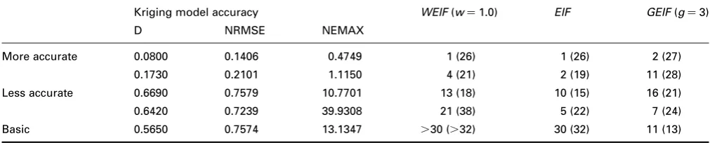
For each test function, four kriging models, two of high accuracy and two of low accuracy, were used with each of the utility functions to locate the optimum to within a certain tolerance. An additional kriging model, constructed using only two design points selected at random, and so naturally of low accuracy, was also used. The results are shown inTables 1–3.

The models are separated in each table according to their accuracy (with the model constructed from just two points labelled as Basic). The number of iterations taken by each utility function to locate the optimum within the required tolerance is given, with the figures in parentheses giving the total number of function evaluations needed, that is the number of iterations taken by the utility function plus the number of experiments used to construct the kriging model. In each case, the stopping criteria used the relative

tolerance, defined as

relative tolerance

¼100

sampled objective function value true minimum

true minimum 0

B B @

1 C C A ð16Þ

A 1% relative tolerance was used for the Humps and Hartman3 test functions, and a 2% relative tolerance was used for the Branin test function.

Two main points can be made regarding the results

(a) Although, in general, fewer iterations may be required when more accurate kriging models are used, this is not always the case.

(b) Even when fewer iterations are required by the utility functions when more accurate kriging models are used, this can come at a cost of a higher total number of objective function evaluations needed.

The first point can be explained as follows: experimental designs may be found that will yield surrogate models which approximate the true function to a high degree of accuracy; however, unless the true function being modelled is actually known and available for comparison, the true accuracy will not be known, and so the kriging model con-structed will have an uncertainty associated with it, no matter how accurate it actually is. It is this uncertainty that the utility function considers when selecting where to sample next. If the true function were available for compari-son, so that the true accuracy of the kriging model could be determined, as in this investigation, then, through the con-struction of a perfectly accurate kriging model, any sub-sequent considerations of uncertainty would become redundant. Therefore the use of utility functions with highly accurate kriging models does not necessarily yield an advantage over the use of utility functions with less accu-rate initial kriging models, as the utility function considers there to be uncertainty present in both models. Nevertheless, the overall trend is that fewer iterations are required by utility functions if they are used with kriging models of higher accuracy.

[image:9.595.49.554.673.776.2]

The second point is more obvious. Although utility func-tions did show an overall trend in locating the optimum of the test functions in fewer iterations, when the kriging model they started with was of higher accuracy, the higher accuracy in the kriging model usually came at the expense of more objective function evaluations being per-formed in the experimental design stage, and this extra cost was not always justified. Each objective function evalu-ation in the experimental design stage is only justified if it

Table 1: Number of Iterations required by WEIF, EIF and GEIF utility functions to locate global minimum within 1% relative tolerance for Humps test function, using kriging models of varying degrees of accuracy

Kriging model accuracy WEIF(w¼1.0) EIF GEIF(g¼3)

D NRMSE NEMAX

More accurate 0.1592 0.4882 4.8411 4 (18) 2 (16) 3 (17)

0.1611 0.6836 2.2516 3 (17) 3 (17) 4 (18)

Less accurate 0.5791 0.8810 32.1664 4 (9) 10 (15) 7 (12)

0.5117 0.7998 23.2252 8 (16) 19 (27) 19 (27)

(10)

means that at least one less iteration will be required by the utility function to locate the optimum.

As the overall aim in single-objective optimisation is to locate the global minimum using as few objective function evaluations as possible, the most attractive experimental design is not the design that yields the most accurate kriging model, but instead the design that leads to the con-struction of a kriging model of such an accuracy that, when the number of additional objective function evaluations needed by the utility function to locate the optimum is added to its size, this number (the total number of objective function evaluations) is minimised. For the three test func-tions given, this was achieved not by use of an experimental design that yielded an accurate model, but instead by use of designs that yielded models of lower accuracy. In fact, for two of the three test functions, the lowest total number of objective function iterations required to locate the optimum to the required tolerance was achieved with a trivial experimental design of just two random points. When the overall aim is to locate the optimum of a function using a surrogate model in as few iterations as possible, it would appear that it is advantageous to start the iterative search early with a relatively inaccurate model.

5 Conclusions

Surrogate-assisted optimisation can be viewed as consisting of two stages: construction of the initial surrogate model through off-line learning, followed by an iterative optimis-ation search with on-line learning. Typically, an experimen-tal design is used to construct the initial kriging model, with the aim of yielding the most accurate surrogate model poss-ible, and utility functions with in-built uncertainty consider-ations are then used to search for the optimum.

The performances of several utility functions were inves-tigated on three test functions, using experimental designs that yielded kriging models of high accuracy, and they were compared with the performances when experimental designs were used that yielded kriging models of lower accuracy. When the aim is to reduce the overall number

of objective function evaluations required to locate the optimum (which is normally the case in practical design optimisation), it was found that no advantage is necessarily achieved by the use of experimental designs that yield more accurate surrogate models, and that a saving in total iter-ations can even sometimes be made if the utility function is allowed to build up the model entirely by itself as it searches for the optimum through on-line learning. For scenarios where objective functions are expensive to compute, such as in electromagnetic design, such a reduction in objective function evaluations is highly desirable.

6 References

1 Canova, A., Freschi, F., and Repetto, M.: ‘Hybrid method coupling AIS and zeroth order deterministic search’, COMPEL Int. J. Comput. Math. Electr. Electron. Eng., 2005, 24, (3), pp. 784 – 795

2 Di Barba, P., Farina, M., and Savini, A.: ‘Multiobjective design optimization of real-life devices in electrical engineering: a cost-effective approach’. (Lecture Notes in Computer Science, (Springer, 2001), pp. 560 – 573

3 Aslett, R., Buck, R.J., Duvall, S.G., Sacks, J., and Welch, W.J.: ‘Circuit optimization via sequential computer experiments: design of an output buffer’,Appl. Stat., 1998,47, pp. 31 – 48

4 Queipo, N.E., Haftka, R.T., Shyy, W., Goel, T., Vaidyanathan, R., and Tucker, P.K.: ‘Surrogate-based analysis and optimization’, Progr. Aerosp. Sci., 2005,41, pp. 1 – 28

5 Lebensztajn, L., Marretto, C.A.R., Costa, M.C., and Coulomb, J.-L.: ‘Kriging: a useful tool for electromagnetic devices optimization’,

IEEE Trans. Magn., 2004,40, (2), pp. 1196 – 1199

6 Jones, D.R.: ‘A taxonomy of global optimization methods based on response surfaces’,J. Glob. Optim., 1998,13, pp. 455 – 492 7 Sykulski, J.K., Al-Khoury, A.H., and Goddard, K.F.: ‘Minimal

function calls approach with on-line learning and dynamic weighting for computationally intensive design optimization’,IEEE Trans. Magn., 2001,37, (5), pp. 3423 – 3426

8 Haykin, S.: ‘Neural networks: a comprehensive foundation’ (Pearson, 1999)

9 Coulomb, J-L., Kobetski, A., Costa, M.C., Marechal, Y., and Jonsson, U.: ‘Comparison of radial basis function approximation techniques’,

COMPEL Int. J. Comput. Math. Electr. Electron. Eng., 2003,22, (3), pp. 616 – 629

[image:10.595.42.548.55.157.2]

10 Farina, M., and Sykulski, J.K.: ‘Comparitive study of evolution strategies combined with approximation techniques for practical

Table 2: Number of iterations required by WEIF, EIF and GEIF utility functions to locate global minimum within 2% relative tolerance for Branin test function, using kriging models of varying degrees of accuracy

D NRMSE NEMAX

More accurate 0.0684 0.2072 3.4690 6 (23) 27 (44) 18 (35)

0.1133 0.1176 1.6552 .30 (.43) 9 (22) 17 (30)

Less accurate 0.6113 0.6578 3.9200 15 (27) 14 (26) 27 (39)

0.6328 0.6815 5.6191 13 (21) 21 (29) 30 (38)

Basic 0.5596 0.6885 27.4274 30 (32) 17 (19) .30 (.32)

Table 3: Number of iterations required by WEIF, EIF and GEIF utility functions to locate global minimum within 1% relative tolerance for Hartman3 test function, using kriging models of varying degrees of accuracy

D NRMSE NEMAX

More accurate 0.0800 0.1406 0.4749 1 (26) 1 (26) 2 (27)

0.1730 0.2101 1.1150 4 (21) 2 (19) 11 (28)

Less accurate 0.6690 0.7579 10.7701 13 (18) 10 (15) 16 (21)

0.6420 0.7239 39.9308 21 (38) 5 (22) 7 (24)

[image:10.595.42.548.215.317.2]

(11)

electromagnetic optimization problems’,IEEE Trans. Magn., 2001, 37, (5), pp. 3216 – 3220

11 Jones, D.R., Schonlau, M., and Welch, W.J.: ‘Efficient global optimization of expensive black-box functions’, J. Glob. Optim., 1998,13, pp. 455 – 492

12 Siah, E.S., Sasena, M., Volakis, J.L., Papalambros, P.Y., and Wiese, R.W.: ‘Fast parameter optimization of large-scale electromagnetic objects using DIRECT with kriging metamodeling’, IEEE Trans. Microw. Theory Tech., 2004,52, (1), pp. 276 – 285

13 Montgomery, D.: ‘Design and analysis of experiments’ (John Wiley and Sons, 2001)

14 Kleijnen, J.P.C., Sanchez, S.M., Lucas, T.W., and Cioppa, T.M.: ‘A user’s guide to the brave new world of designing simulation experiments’, INFORMS J. Comput., 2005, 17, (3), pp. 263 – 289

15 Liu, L., and Wakeland, W.: ‘Does more uniformly distributed sampling generally lead to more accurate prediction in computer experiments?’. Proc. 2005 Winter Simulation Conf. 2005, Kuhl, M.E., Steiger, N.M., Armstrong, F.B., and Joines, J.A. (Eds.), pp. 2561 – 2571

16 McKay, M.D., Conover, W.J., and Beckman, R.J.: ‘A comparison of three methods for selecting values of input variables in the

analysis of output from a computer code’,Technometrics, 1979,21, pp. 239–245

17 Kalagnanam, J.R., and Diwekar, U.M.: ‘An efficient sampling technique for off-line quality control’,Technometrics, 1997,39, (3), pp. 308 – 319

18 Wilkinson, J.H.: ‘Rounding errors in algebraic processes’ (Prentice-Hall, Englewood Cliffs, NJ, 1963)

19 ‘Matlab, computation High-performance numeric guide visualization software. Reference Guide’ (The Math Works Inc., Natick, MA, 2004)

20 Dixon, L.C.W., and Szego, G.P.: ‘The global optimisation problem: an introduction’ in Dixon, L.C.W., and Szego, G.P. (Eds.): ‘Towards global optimisation’ (North-Holland, Amsterdam, 1978), Vol. 20, pp. 1 – 15

21 Hartman, J.K. Tech. Rept. NP55HH72051A, Naval Postgraduate School, Monterey, CA, 1972

22 Schonlau, M., Welch, W.J., and Jones, D.R.: ‘Global versus local search in constrained optimization of computer models’, IMS Lecture Notes, 1998,34, pp. 11 – 25