Incomplete split plots in variety trials based on a designs

Paper in BIULETYN OCENY ODMIAN. 2003. Vol 31, p 7-16

KRISTIAN KRISTENSEN

Biometry Research Unit

Department of Agricultural Systems Danish Institute of Agricultural Sciences

Incomplete split-plots in variety trials - based on

α

-designs

Summary

Incomplete split-plots based on α-designs are proposed as alternative to traditional split-plot designs. The purpose of the incomplete split-plot designs is to increase the efficiency of the treatment (whole plot factor) comparisons especially for specific varieties. The designs are constructed using 4 different methods, but in all methods the units for the treatments are the incomplete blocks (instead of whole plots with all varieties in traditional split-plots). The designs are compared with each other and with traditional split-plot and randomised complete block designs using generated data with known covariance structure and using data from 5 uniformity trials. The comparisons showed that these designs in almost all cases were more efficient than the traditional designs and that they were never considerably less efficient that these. Designs where the incomplete blocks are grouped so that each group contain all treatments (one incomplete block with each treatment) were more efficient that when the incomplete blocks were randomised independently.

Keywords

α-designs, uniformity trials, efficiency of designs, variety trials.

Introduction

In order to evaluate new varieties it is often relevant to examine the varieties under different circumstances, such as with and without chemical control of fungal diseases or at low and high nitrogen input level. In such situations the split-plot designs are often used because it is then very easy to apply the circumstances (hereafter called treatments) under which the varieties has to be examined. The split-plot is also very efficient for comparing a low number

of varieties at each of the different treatments. However, when many varieties are to be compared a simple split-plot is inefficient and some types of incomplete blocks are then often used within each whole-plot. When using split-plots the efficiency of comparing the varieties response to the different treatments is very low, partly because only few degrees of freedom are present in the whole plot stratum and partly because the random variation between whole plots usually are large. During the last years there has been an emerging interest to compare the varieties sensibility to different treatments. In that case the split-plot is inefficient. This could of course be solved by randomising the individual combinations of treatments and varieties, but from a practical point of view this would be difficult to manage and in most situations would also require a larger part of the area to be used as guard plots which will increase the area to use and could subsequently increase the random variation. The present paper describes some possible alternatives to split plot. They can be regarded as a

compromise between the traditional split-plot and the randomised complete block designs.

Designs

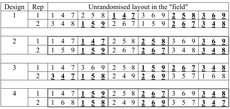
The suggested designs are based on α-designs (Patterson and Williams, 1976). The designs are constructed in four different ways (table 1).

Table 1 The layout of the four designs exemplified by a trial with 2 replicates, 9

varieties and 2 treatments based on an alpha design with r=2 (design 1 and 2) or r=4

(design 3 and 4), v=9, s=3 and k=3. In design 2 and 4 the blocks are collected in

groups - one with each treatment. In design 1 and 3 the blocks are randomised independently. (The groups are surrounded with double lined frames and blocks separated by single lines). Varieties are given by figures and the two treatments are

given by ±bould and ±underlining.

Design Rep Unrandomised layout in the "field"

1 1 1 4 7 2 5 8 1 4 7 3 6 9 2 5 8 3 6 9

2 3 4 8 1 5 9 2 6 7 1 5 9 2 6 7 3 4 8

2 1 1 4 7 1 4 7 2 5 8 2 5 8 3 6 9 3 6 9

2 1 5 9 1 5 9 2 6 7 2 6 7 3 4 8 3 4 8

3 1 1 4 7 3 6 9 2 5 8 1 5 9 2 6 7 3 4 8

2 3 4 7 1 5 8 2 4 9 2 6 9 3 5 7 1 6 8

4 1 1 4 7 1 5 9 2 5 8 2 6 7 3 6 9 3 4 8

2 1 6 8 1 5 8 2 4 9 2 6 9 3 5 7 3 4 7

In the first two methods the blocks of a traditional α-design with r replicates is copied as many times as the number of treatments in the trial. So if two treatments are planned each replicate consist of two identical sets of blocks. In general each replicate will contain ts

second method the blocks are randomised in two steps: 1) the s groups of t identical blocks are randomised within each replicate, 2) the t blocks (with treatments 1, 2,…, t) are

randomised within each group of identical blocks.

In the last two methods the blocks of a traditional α-designs with tr replicates are used. The blocks in r of the replicates are assigned to treatment 1, the blocks in another set of r

replicates are assigned to treatment 2 and so on until the last r replicates are assigned to treatment t. The original tr replicates of the α-design are then collected in order to form r

complete replicates (each containing all combinations of varieties and treatments). In the third method the ts blocks are randomised independently within each of these replicates. In the fourth method the blocks are collected in s groups so that each group contain one block with each of the t treatments; then the s groups are randomised within each replicate and finally the

t blocks (with treatments 1, 2,…, t) are randomised within each group of blocks.

The way of construction and randomisations suggest two different models to be used for the analysis of such designs. These two models are shown below - together with models for traditional split plot and randomised complete block designs:

( ) Split-plot

( ) Randomised complete block

( ) Design 1 and 3

( ) Design 2 and 4

where

rtv v t vt r rt rtv

rtv v t vt r rtv

rbtv v t vt r rb rbtv

rgbtv v t vt r rg rgb rgbtv

Y A B E

Y A E

Y A D E

Y A C D E

Y

µ δ τ δτ

µ δ τ δτ

µ δ τ δτ

µ δ τ δτ

= + + + + + +

= + + + + +

= + + + + + +

= + + + + + + +

, or is the yield of variety with treatment (in block of group ) in replicate , , ,( , ) and ( , , ) is the the effect of replicate, whole plot, group of b

rtv rbtv rgbtv

r rt rg rb rgb rtv rbtv rgbtv

Y Y v t b g r

A B C D D E E E

t

locks, blocks and plots, respectively is the effect of variety

is the effekt of treatment

( ) is the interaction effect of variety with treatment , and ( ) are systematic effects

v t vt v vt v t v t A δ τ δτ

δ τ δτ

, , ,( , ) and ( , , ) are regarded as random effects, although A and may be treated as fixed effects

The random effects are asumed to be iid normally distributed each with

r rt rg rb rgb rtv rbtv rgbtv r

rg

B C D D E E E

C

2 2 2 2 2

mean value 0 and variances σ σ σ σ_A, _B, _C, _D and σ_E, respectively

Efficiency of the designs

fields for each type of pair wise comparison and design. The trials used for evaluation had 80 varieties, which were to be compared at 2 different treatments. The trials were laid out with 2 replicates and the α-designs used had a block size of 8 plots. The efficiency factor of the α -designs was 0.8058 and 0.8642 for -designs based on 2 and 4 replicates, respectively.

Using generated data

The generated data were assumed to consist of 4 columns with 80 plots in each column. Each replicate were assumed to consist of 2 columns. The 80 plots in each column were subdivided in 10 incomplete blocks of 8 plots each. Pairs of blocks were formed by the 2 blocks located side-by-side in column 1 and 2 (in replicate 1) or column 3 and 4 (in replicate 2). I the split-plot each column within replicates formed a whole split-plot. Each split-plot was assumed to be 10 m by 1 m, so that the total area was 80 m by 40 m. The data was generated using the following three covariance structures:

2

/ 20 2

/ 200 2

2 ii

10 0 Independent observations 10 9 Quickly decreasing covariance 10 9 Slowly decreasing covariance where

is the variance on point is the covariance between

ij

ij

ii ij

d

ii ij

d

ii ij

ij

e e

i

σ σ

σ σ

σ σ

σ σ

−

−

= =

= =

= =

point and is the distance between point and

ij

i j

d i j

Based on these, the variance components were calculated for each design using the theory of regionalized variables as described by Journel and Huijbregts (1978) and as used by

Kristensen and Ersbøll (1992). Finally the variance components were adjusted by a factor, so that the sum of variance components was fixed to 10. The factors were 1.52 and 8.63 for the quick and slow decreasing covariance, respectively. The variance components are shown in the top part of table 8, except the variance component for replicate, which was 0.85 and 1.24 for fields with quick and slow decreasing covariance, respectively.

Using uniformity trials

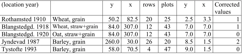
Data from five different uniformity trials was investigated. The trials were all grown with cereals. An overview of the trials is given in table 2. The first uniformity trial was carried out at Rothamsted in 1910 (Mercer & Hall, 1911) and had almost quadratic plots. The next two trials were from 1918 and 1920, respectively - both from the same field at the Danish experimental station Blangstedgaard. Those two trials have been analysed previously by Dorph-Petersen (1949). The plots were rather large and quadratic. The fourth and the fifth trial were more recent uniformity trials at two Danish experimental stations, Jyndevad and Tystofte. These trials have been described by Heidmann (1988 and 1989) and by Kristensen and Ersbøll (1995). In the more resent trials the plots were rectangular with a width of 1.5 m and a length of 8.5-9.0 m.

Table 2 Crop, recorded variable and dimension of uniformity trials

(location year) y x rows plots y x Corrected values Rothamsted 1910 Wheat, grain 50.2 82.5 20 25 2.5 3.3 1 Blangstedgd. 1918 Wheat, straw+grain 84.0 307.0 12 43 7.0 7.0 1 Blangstedgd. 1920 Oat, straw+grain 84.0 307.0 12 43 7.0 7.0 0 Jyndevad 1987 Barley, grain 260.0 30.0 26 20 8.5 1.5 2 Tystofte 1993 Barley, grain 58.0 70.5 4 47 9.0 1.5 0

As all uniformity trials were used for evaluating the same designs only a part (the top left part) of the uniformity trials were selected for the study. The selected part of the trials is shown in table 3. (Note that for Tystofte only 1 replicate could be accommodated).

Table 3 Dimension, mean and standard deviation of the part of the uniformity trials in the calculations

Field size, m Number of Uniformity trial

(location and year) y x rows plots Mean,

hkg ha-1 hkg haStd. , -1 Rothamsted 1910 50 52.8 20 16 40.4 4.7 Blangstedgd. 1918 56 280 8 40 51.0 7.2 Blangstedgd. 1920 56 280 8 40 42.0 2.9 Jyndevad 1987 200 24 20 16 32.8 4.4

Tystofte 1993 58 60 4 40 33.5 5.4

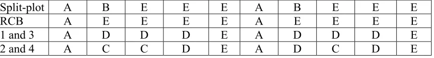
The layout of replicates, groups (pairs) of blocks and blocks were done in two different ways - depending on the size of the uniformity trials. The two methods are shown in table 4 and 5.

Table 4 Layout of replicates, blocks, groups (pairs) of blocks and whole plots for the designs to be compared using the uniformity trials at Blangstedgaard and Tystofte. The figures in the body of the table are block numbers. Each block had 8 plots in 1 column. The replicates, whole plots and the top/left coordinates of the blocks (in plot numbers) are shown in the row and column headings.

Rep 1 2

Whole plot 1 2 1 2

top/left 1 2 3 4 5 6 7 8

1 1 1 6 6 1 1 6 6

9 2 2 7 7 2 2 7 7

17 3 3 8 8 3 3 8 8

25 4 4 9 9 4 4 9 9

33 5 5 10 10 5 5 10 10

column. The replicates, whole plots and the top/left coordinates of the blocks (in plot numbers) are shown in the row and column headings.

Rep 1 2

Whole

plot top/left 1 2 3 4 5 6 7 8 9 10 11 12 13 14 15 16 17 18 19 20

1 1 1 2 3 4 5 6 7 8 9 10 1 2 3 4 5 6 7 8 9 10

2 9 1 2 3 4 5 6 7 8 9 10 1 2 3 4 5 6 7 8 9 10

For each of the uniformity trials a random effect model were set up in order to estimate a set of variance components to be used for calculating the standard deviations on the pair wise comparisons

The models were:

( ) ( ) ( ) ( ) ( ) ( ) ( ) ( ) ( ) ( ) ( ) ( ) ( ) ' ' ' ' ' ' ' ' ' where

is the recorded yield in plot is the overal mean

is the effect of replicate applied to plot is the effect

i i i i i i i i i i

i

i i

i r w r g w r b g w r i

i

r

w r

Y A B C D E

Y i

A r i

B µ µ = + + + + + ( ) ( ) ( ) ( ) ( ) ( ) ( ) ' '

of wholeplot within replicate applied to plot

is the effect of group of blocks within wholeplot of replicate applied to plot is the effect of block with

i i i

i i i i

g w r

b g w r

w r i

C g w r i

D b

( ) ( ) ( ) ( ) ( ) ( ) ( ) ( ) ( ) ( )

' i

' ' ' ' '

in group in wholeplot of replicate applied to plot E is the residual effect of plot , i.e. the effect of plots within blocks

, , , and is as

i i i i i i i i i i

r w r g w r b g w r i

g w r i

i

A B C D E

2 2 2 2 2

sumed to be iid normally distributed with mean value 0 and variances ,θ θ θ θ_{A B}, _C, _D andθ_E, respectively

Based on these variance components the variance components for the relevant effects in the individual designs were estimated by adding the relevant θi2 values. Table 6 show for each design how the variance components for replicates (A), whole plots (B), groups of blocks (C), Blocks (D) and plots (E) are estimated from the variance components of the uniformity trials. E.g. the residual variance for the randomised complete block design (RCB) is calculated as the sum: θB2+θC2+θD2+θE2. Then average variance for all differences of treatment main effects, variety main effects, treatment differences within each variety and variety differences within each treatment was calculated and an approximate average degree of freedom was calculated for the same differences. Based on these the "average" Lsd value for each comparison was finally calculated.

Table 6 List of how the variance components estimated from the uniformity trials enters into the variance components of the different designs

Blangstedgaard and Tystofte Rothamsted and Jyndevad Design

Split-plot A B E E E A B E E E RCB A E E E E A E E E E

1 and 3 A D D D E A D D D E

2 and 4 A C C D E A D C D E

Results

The variance components for each uniformity trials are shown in table 7. The variability varies greatly from field to field being smallest at Blangstedgaard in 1920 and largest in the same field in 1918. Also the distribution of the variability on the different components differs greatly from trial to trial. At Rothamsted 1910 almost all the variability was found in the component for plots indicating that the correlation between neighbouring plots was close to zero at this location. On the other extreme, at Tystofte 1993, only 20% of the total variation was between plots within blocks, which indicates that the correlations between plots in the same block (of 8 plots) was high.

Table 7 Variance components estimated from the uniformity trials

Variance components Field θA2 θB2 θC2 θD2 θE2

Total

Rothamsted 1910 0 0.98 0.03 0 21.11 22.12 Blangstedgaard 1918 20.46 1.27 13.85 5.84 21.61 63.03 Blangstedgaard 1920 0 0.78 0 4.32 3.64 8.74 Jyndevad 1987 0.08 2.47 2.79 0.36 14.03 19.73 Tystofte 1993 - 3.81 0 21.76 6.35 31.92

Based on these field components, the variance components for calculating the efficiency of the different designs was formed (bottom part of table 8). The variance components for the generated fields are shown in the top part of table 8.

Table 8 Estimates of variance components that are of importance for comparing treatments and varieties for each design

Design Split-plot RCB 1 and 3 2 and 4 Field σB2 σE2 σE2 σD2 σE2 σC2 σD2 σE2

Generated:σij=0 0.00 10.00 10.00 0.00 10.00 0.00 0.00 10.00

Generated:σij=9e-d/20 0.30 8.85 9.15 8.41 0.75 7.07 1.33 0.75

Generated:σij=9e-d/200 0.45 8.31 8.76 8.26 0.50 7.16 1.09 0.50

Rothamsted 1910 0.98 21.14 22.12 1.01 21.11 0.03 0.98 21.11 Blangstedgaard 1918 1.27 41.30 42.57 20.96 21.61 15.12 5.84 21.61 Blangstedgaard 1920 0.78 7.96 8.74 5.10 3.64 0.78 4.32 3.64 Jyndevad 1987 2.47 17.18 19.65 5.62 14.03 2.79 2.84 14.03 Tystofte 1993 3.81 28.11 31.92 25.57 6.35 3.81 21.76 6.35

designs, design 2 and 4 usually showed the smallest Lsd-values. Only in the generated fields with independent observations and in the Rothamsted field had design 1 and 3 smaller Lsd-values than design 2 and 4. In all fields all the alternative designs were clearly better than the split-plot design. For several fields, the alternative designs decreased the Lsd-value by a factor 10 or more - when compared to the split-plot.

Table 9 Estimated average Lsd.95-values for comparing differences between

treatment main effects in each design

Generated fields Uniformity fields Design

σij= 0

σij= 9e-d/20

σij= 9e-d/200

Roth.

1910 Blgd. 1918 Blgd. 1920 Jynd. 1987 Tyst. 1993

DF, Used (and range)

Split-plt. 4.49 8.14 9.45 14.18 16.99 11.92 20.83 25.93 1 (1-1)

RCB 0.71 0.47 0.46 1.04 1.44 0.65 0.98 1.25 159(159-159) 1 (r Indp.) 0.74 1.91 1.89 1.25 3.19 1.55 1.78 3.37 22 (26-32)

2 (r Grp.) 0.76 0.81 0.73 1.29 1.98 1.49 1.45 3.22 14 (11-32)

3 (rt Indp) 0.74 1.91 1.89 1.25 3.19 1.55 1.78 3.37 22 (14-31)

4 (rt Grp) 0.76 0.81 0.73 1.29 1.98 1.49 1.45 3.22 14 ( 5-31)

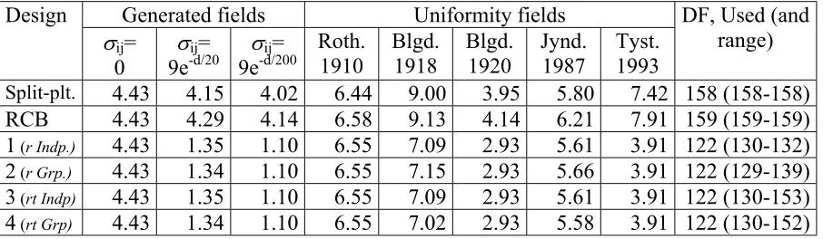
For the comparison of variety main effects (table 10) all the alternative designs gave a smaller Lsd-value than both the split plot and the randomised compete block design, except in the generated fields with independent observations and the Rothamsted field (were the difference is zero or very small). The reason for these low Lsd-values must be due to the use of

incomplete block designs. The reduction was most pronounced in the Tystofte field where the Lsd-value was reduced to approximately 50%. For the generated fields with decreasing covariance the reductions were even higher.

Table 10 Estimated average Lsd.95-values for comparing differences between variety

main effects in each design

Generated fields Uniformity fields Design

σij= 0

σij= 9e-d/20

σij= 9e-d/200

Roth.

1910 Blgd. 1918 Blgd. 1920 Jynd. 1987 Tyst. 1993

DF, Used (and range)

Split-plt. 4.43 4.15 4.02 6.44 9.00 3.95 5.80 7.42 158 (158-158)

RCB 4.43 4.29 4.14 6.58 9.13 4.14 6.21 7.91 159 (159-159) 1 (r Indp.) 4.43 1.35 1.10 6.55 7.09 2.93 5.61 3.91 122 (130-132)

2 (r Grp.) 4.43 1.34 1.10 6.55 7.15 2.93 5.66 3.91 122 (129-139)

3 (rt Indp) 4.43 1.35 1.10 6.55 7.09 2.93 5.61 3.91 122 (130-153)

4 (rt Grp) 4.43 1.34 1.10 6.55 7.02 2.93 5.58 3.91 122 (130-152)

Table 11 Estimated average Lsd.95-values for comparing differences between

treatment effects for each variety in each design

Generated fields Uniformity fields Design

σij= 0

σij= 9e-d/20

σij= 9e-d/200

Roth. 1910

Blgd. 1918

Blgd. 1920

Jynd. 1987

Tyst. 1993

DF, Used (and range)

RCB 6.26 5.99 5.86 9.31 12.92 5.85 8.78 11.19 159 (159-159) 1 (r Indp.) 6.27 2.63 2.38 9.28 10.42 4.37 8.06 6.36 122 (141-151)

2 (r Grp.) 6.27 2.03 1.67 9.28 9.85 4.33 7.85 6.24 122 (137-153)

3 (rt Indp) 6.27 2.63 2.38 9.28 10.42 4.37 8.06 6.36 122 (152-156)

4 (rt Grp) 6.27 2.03 1.68 9.28 10.03 4.34 7.96 6.24 122 (143-154)

The Lsd-values for comparing two treatments for a specific variety (table 11) did not vary as much as that for the treatment main effects. The largest differences were found for the trials based on generated data with non-zero covariance. Here the Lsd-values were reduced by 56%-72% when compared to the split-plot. For the uniformity fields the reduction was greatest for the field at Tystofte and smallest for the field at Rothamsted. For the best alternative designs (design 2 and 4) the reduction varied between 1% and 45% when compared to the split-plot.

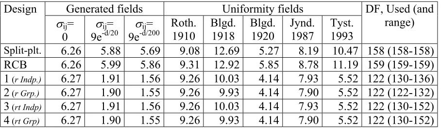
An almost similar picture was seen for the comparison of two varieties at a given treatment (table 12). However, for fields at Rothamsted and the generated field with independent observations the split-plot had a slightly smaller (0.2%-2%) Lsd-value than the alternative designs. For the uniformity fields the reduction varied between -2% and 47% with the largest reduction at Tystofte.

Table 12 Estimated average Lsd.95-values for comparing differences between variety

effects for each treatment in each design

Generated fields Uniformity fields Design

σij= 0

σij= 9e-d/20

σij= 9e-d/200

Roth. 1910

Blgd. 1918

Blgd. 1920

Jynd. 1987

Tyst. 1993

DF, Used (and range)

Split-plt. 6.26 5.88 5.69 9.08 12.69 5.27 8.19 10.47 158 (158-158)

RCB 6.26 5.99 5.86 9.31 12.92 5.85 8.78 11.19 159 (159-159) 1 (r Indp.) 6.27 1.91 1.56 9.26 10.03 4.14 7.93 5.52 122 (130-136)

2 (r Grp.) 6.27 1.90 1.55 9.26 9.93 4.14 7.90 5.52 122 (122-132)

3 (rt Indp) 6.27 1.91 1.56 9.26 10.03 4.14 7.93 5.52 122 (130-152)

4 (rt Grp) 6.27 1.90 1.55 9.26 9.93 4.14 7.90 5.52 122 (130-152)

Discussion

The alternative designs prevent the user from calculating the intra-block variety estimates because the block effects must be random in order to estimate the random variation to be used for testing the treatment effects. This may be regarded as a disadvantage in cases where harvesting - or other processes has to be interrupted within a whole replicate. However this would also be a problem with the traditional split-plot. In design 2 and 4 it is possible to treat the pairs of blocks as fixed effects and thus interrupt a handling process at the border between two groups of blocks

small increase could be expected in cases where the variance component for groups of blocks are zero (or close to zero). In cases where the variation between groups of blocks is expected to be considerable larger than the variation between blocks within groups it should be

beneficial to group the blocks.

When grouping of blocks is to be used it seems most logical to base the design on t (t is the number of treatments) identical α-designs each with the required number of replicates as this excludes any partial confounding between varieties and treatments.

The alternative designs may require more guard areas between treatments than the split-plot designs. The larger guard areas may decrease the benefit from using these, partly because more land is needed and partly because the increased area for the trial may also increase the random variation.

The alternative designs are more difficult to handle in the field because they require the treatments to be applied on more (and smaller) pieces of lands. A compromise between the increase in treatment (and variety) comparisons and the increased workload may be obtained by choosing a suitable size of the incomplete blocks. Large block sizes will decrease the additional workload as the number of blocks - and thus the number of different pieces of land to be treated - will decrease. However, too large blocks will have a negative effect on the efficiency of the comparisons as the residual variation is expected to increase. In addition large block sizes will decrease the number of degrees of freedom for testing the treatment effects.

Conclusion

The efficiency of treatment and variety comparisons in traditional split-plot designs can be increased by an alternative layout based on α-designs. The efficiency of the treatment main effect comparisons was increased very much under all examined circumstances. The

efficiency of the other comparisons (treatment comparisons for specific varieties, variety main effect comparisons and variety comparisons at specific treatments) was also increased in most cases and was never considerably less efficient than when traditional split-plot designs were used.

Designs where the incomplete blocks are grouped and randomised in two steps were usually more efficient (and newer less efficient) than designs were the incomplete blocks were randomised independently.

References

Dorph-Petersen, K. 1949. Parcelfordeling i markforsøg. Tidsskrift for Planteavl. 52, 111-175

Heidmann, T. 1988. Startkarakterisering af arealer til systemforskning: I Forsøgsarealer, måleprogram og metoder. Tidsskrift for Planteavls Specialserie. S 1958, 89 pp.

Heidmann, T. 1989. Startkarakterisering af arealer til systemforskning: IV Resultater fra arealet ved Jyndevad. Tidsskrift for Planteavls Specialserie. S 2021, 163 pp.

Kristensen, K. and Ersbøll, A. K. 1992. The Use of Geostatistical Methods in planning variety trials. Forth Working Seminar on Statistical methods in Variety Testing. Biuletyn Oceny Odmian (Cultivar testing Bulletin). 24-25, 139-157.

Kristiensen, K. and Ersbøll, A.K. 1995. The use of Geostatistical methods in variety trials, where some varieties are unreplicated. Biuletyn Oceny Odmain (Cultivar Testing Bulletin), 26-27, 113-122.

Mercer, W. B. and Hall, A. D. 1911. The experimental error of field trials. Journal of Agricultural Science (Cambridge). 4, 107-132.