Elastostatic interaction analysis of frames resting on homogeneous elastic half space

(1)

Elastostatic Interaction Analysis of Frames

Resting on Homogeneous Elastic Half-space

By

Reza Izadnegandar

Submitted in fulfillment of the requirements

for the Degree of Master of Engineering Science

University of Tasmania

(2)

UNIVERSITY OF TASMANIA

C;_3.) c I ck—d-

School of Engineering

Elastostatic

Interaction Analysis

of Frames Resting on

Homogeneous Elastic Half-space

Master of Engineering Science Thesis

(3)

ORIGINALITY

This thesis contains no material which has been accepted for a degree or diploma by the University of Tasmania or any other institution, except by way of background information and duly acknowledged in the thesis, and to the best of the candidate's knowledge and belief no material previously published or written by another person except where due knowledgment is made in the text of the thesis.

Signed:

(Reza Izadnegandar)

AUTHORITY OF ACCESS

(4)

ABSTRACT

The structural response of a building to applied loads depends on the behaviour of the soil supporting the structure. Structures may undergo various support deflections dependant on their support conditions. Such deflections are associated with soil deformation: the short-term deflections are known as the elastic component and, the long-term deflections are known as the permanent plastic component. Differential support displacements cause structural interaction between supports.

To analyse such interaction, there are different approaches; it can be analytical or numerical, static or dynamic and deterministic or probabilistic, with the rigour in the analysis being commensurate to the degree of displacement likely to be experienced. Mathematical rigour, however, may or may not be justified if inadequate knowledge of parameters exists. In the context of the natural variability of constituent parameters, a closer examination of the soil parameters associated with this interaction, particularly for plane frame structures, is warranted.

The behaviour of soil media at a structure's supports during structural analysis has been the focus of much investigation and research over the last century. Efforts have been made to describe such interaction and many computer packages have been developed to incorporate different soil models with the structural studies. Unfortunately the models are usually too complex or require too much input data for easy use by professional engineers.

(5)

A displacement-type analytical-numerical technique of elastic solution is used to evaluate support interaction. In this approach, the behaviour of soil is modelled by means of homogenous, elastic half-space, whilst in the analysis of the structure, a Direct Stiffness Method is applied.

The Boussinesq and Cerruti force-displacement solutions are used for isotropic behaviour, whilst the Gerrard-Wardle and Gerrard-Harrison models are used for cross-anisotropic behaviour. The flexibility matrix of the elastic half-space, related to the interaction forces is developed. The author has prepared an integrated software program to perform the analysis on a desktop PC.

(6)

NOTATIONS

Flexibility coefficient with superscripts a and b denoting the points of the displacement considered and of the load applied, and where the subscripts i and j designate the directions associated with the displacement and the load, respectively.

Coefficients' positions in an off-diagonal block in a soil flexibility matrix associated with two distinct points

Coefficients' positions in a diagonal block in a soil flexibility matrix associated with two coincident points

Local Cartesian coordinates

u, v, w Displacements in x, y and z directions in subscripts presenting the location of the point considered

X, Y, Z Global Cartesian coordinates

r, 0, z Cylindrical coordinates (radial, tangential and vertical directions)

a, b,c,d, f Components of elasticity tensor for a cross-anisotropic material

g4, hip if •••

ill, ..., S9,

Constants and integration coefficients in Chapters 2 and 3

/200, c/a)°, _s

'200' /702 1722 220

c'220' s *1 220 /420 c'420' s'420' 1422 L000 „. L000 „.L000 , L002, L020,

c L020 s L020 L022 LI 20 '

A₂₂₀ 5M ₂₂₀ _M₂₂₂ _M₄₂₀ _r_M₄₂₀

s M420 P020 S020 / S022 Sl2O S122

Ev, Eh, Young's moduli, shear modulus, and Poisson's ratios in a

F„, cross-anisotropic soil material with symmetry about a vertical axis in vh, v", Voi its elastic properties

E, G, v Young's and shear moduli and Poisson's ratio for an isotropic material

E, G., vs Young's and shear moduli and Poisson's ratio for an isotropic soil Pz, go My Concentrated vertical and horizontal forces and a horizontal moment

Vertical distributed load

(7)

Tension field in a fictitious elastic membrane in two-parameter soil model

D. D_rFlexural rigidity of a foundation plate of general shape, and a circle

E₁₃₁_'_G₃_{. P}_{Young's and shear moduli and Poisson's ratio for a plate}

Radius of circular loading area 0

Modulus of sub-grade reaction in Winkler model

k, K Transform parameters ( K = k ro Chapter 1)

fa(r), fb(r),}

Functions of r corresponding to load stress distributions

f(r)

a, fi,co,y, I

Derived elastic quantities reflecting nature of anisotropy

H 0(k), H1 (k) ilankel transforms of order zero and one

A _Cr1(T)

I crA (IF), tro.A. 9 4.-rA ,

LcrA (1// ), LcrA ,

M crAen, sM CrA ,

S (V) cSN, crA

Integrals involved in the general solutions for displacements, strains and stresses

1, A, I Length, cross-sectional area, the moment of inertia about the z-axis for structure element

[K] Structure stiffness matrix

[Ks] Soil stiffness matrix

[Ksys] System stiffness matrix

kab Element stiffness coefficient

[kabi(e) Stiffness matrix (3x3) for element (e) associated with forces at node a due to displacements of node b

[k 't Local Element stiffness matrix [kt Global element stiffness matrix {Fle Element nodal force vector

(8)

{A} Nodal displacements vector

[TL

Element transformation matrix

[Tier Transpose of element transformation matrix.

{P} Nodal external forces vector {P}° Total fixed end forces vector {R._{,} Reaction forces vector}

{R} Nodal elastic restraint forces vector {Ft Total local element end forces vector

{F}e Vector of local fixed end forces due to the loads applied to an element {F°1 Vector of global fixed end forces due to the loads applied to an

element

(9)

2.3.2 Homogeneous Isotropic Elastic Half-space 26 2.3.2.1 Further Solution Associated with Isotropic Elastic Half-space 29 2.4 CROSS-ANISOTROPIC ELASTIC HALF-SPACE MODELS 32 2.4.1 Points of Load Application and Displacement Distinct 35 2.4.1.1 Displacements due to a Vertical Point Load 36 2.4.1.2 Displacements due to a Horizontal Point Load 37 2.4.1.3 Displacements due to a Moment Load about Horizontal Axis

37 2.4.2 Points of Load Application and Displacement Coincident 38

2.4.2.1 Displacements due to a Vertical Uniform Load .39 2.4.2.2 Displacements due to a Horizontal Uniform Load 40 2.4.2.3 Displacements due to a Vertical Linear Load 40 2.5 NON-HOMOGENEOUS ISOTROPIC ELASTIC HALF-SPACE

(10)

2.6 METHODS OF OBTAINING SOIL PARAMETERS 44 2.7 CONCLUDING REMARKS TO CHAPTER 49

CHAPTER 3 METHOD OF SOLUTION

50

3.1 INTRODUCTION 50

3.2 STRUCTURE-SOIL SYSTEM 50 3.3 DIRECT STIFFNESS MATRIX METHOD 53 3.4 SUPERSTRUCTURE CONTRIBUTION IN ANALYSIS 54 3.4.1 Assumptions in Superstructure analysis 55 3.5 SOIL CONTRIBUTION IN ANALYSIS 55

3.5.1 Assumptions in Soil Consideration 56

3.5.2 Development of Soil Stiffness Matrix 56 3.5.3 Flexibility Coefficients Associated with Two Distinct Points on a

Homogeneous Isotropic Elastic Half-space 58

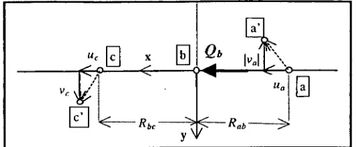
3.5.3.1 Flexibility Coefficients Associated with Horizontal Force Qb 59 3.5.3.2 Flexibility Coefficients Associated with Vertical Force Pb 61 3.5.3.3 Flexibility Coefficients Associated with Moment _Mb about

Horizontal Axis z 63

3.5.4 Flexibility Coefficients Associated with Two Coincident Points on a

Homogeneous Isotropic Elastic Half-space 64

3.5.4.1 Flexibility Coefficients Associated with Horizontal Force Qb 65 3.5.4.2 Flexibility Coefficients Associated with Vertical Force Pb 66 3.5.4.3 Flexibility Coefficients Associated with Moment _Mb about

Horizontal Axis Z 67

3.5.5 Flexibility Coefficients Associated with Two Distinct Points on a

Homogeneous Cross-anisotropic Elastic Half-space 70 3.5.5.1 Flexibility Coefficients Associated with the Displacements due

to Horizontal Load Qb .71

3.5.5.2 Flexibility Coefficients Associated with the Displacements due

to Vertical Load Pb 72

3.5.5.3 Flexibility Coefficients Associated with the Displacements due to Moment _Mb about Horizontal Axis z 73

3.5.6 Flexibility Coefficients Associated with Two Coincident Points on a Homogeneous Cross-anisotropic Elastic Half-space 74 3.5.6.1 Flexibility Coefficients Associated with the Displacements due

to Horizontal Force Qb 75

3.5.6.2 Flexibility Coefficients Associated with the Displacements due

to Vertical Force Pb 76

3.5.6.3 Flexibility Coefficients Associated the Displacements due to

Moment Mb about Horizontal Axis Z 78 3.6 CONCLUDING REMARKS TO CHAPTER 80

CHAPTER 4 SOFTWARE DEVELOPMENT

81

4.1 INTRODUCTION 81

4.2 MODULE "DATAENTR" 89

(11)

4.5 CONCLUDING REMARKS TO CHAPTER 87

CHAPTER 5

EXAMPLES OF ANALYSIS APPLICATIONS 88

5.1 INTRODUCTION 88

5.2 HINGE-SUPPORTED FRAME AND SOIL MODEL APPLIED 88 5.3 EXAMPLES STUDIED IN THIS PROJECT 90

5.3.1 Nomenclature Applicable to Examples, Charts, Graphs and Tables 92 5.3.2 Examples of Analysis of Frame Founded on Isotropic Soil 99 5.3.3 Set One Examples for Cross-anisotropic Soil 106 5.3.4 Set Two Examples, Simulated Cases of Cross-anisotropic Soil 113

5.4 STRUCTURE FOUNDED ON AN INFINITELY RIGID SOIL 117 5.5 STRUCTURE FOUNDED ON WINKLER SOIL 117 5.6 VERIFICATION OF RESULTS OF ANALYSIS 120 5.7 JUSTIFICATION OF THE TYPE OF FRAME AND LOADS

USED IN THE ANALYSES 121 5.8 CONCLUDING REMARKS TO CHAPTER 128

CHAPTER 6

DISCUSSION OF RESULTS 129

6.1 INTRODUCTION 129

6.2 OBSERVATIONS AND DISCUSSIONS ON RESULTS OF ANALYSING FRAME ON ISOTROPIC ELASTIC

HALF-SPACE 129

6.2.1 Case One of an Isotropic Soil 130

6.2.2 Case Two of an Isotropic Soil 134

6.2.3 Comparison of Cases One and Two of the Isotropic Soil 135

6.3 OBSERVATIONS AND DISCUSSIONS ON RESULTS OF ANALYSING FRAME ON CROSS-ANISOTROPIC ELASTIC

HALF-SPACE 136

6.4 FINDINGS AND DISCUSSION ON RESULTS OF ANALYSIS: WINKLER MODEL AS COMPARED WITH ISOTROPIC

ELASTIC HALF-SPACE 145 6.5 SENSITIVITY ANALYSIS 147 6.6 CONCLUDING REMARKS TO CHAPTER 148

CHAPTER 7

SUMMARY AND CONCLUSIONS 150

7.1 SUMMARY 150

7.2 CONCLUSIONS 151

7.3 FUTURE WORK 153

REFERENCES R-1

APPENDICES

APPENDIX Al 1-1

Al VERTICAL DISPLACEMENTS UNDER A LOAD

(12)

APPENDIX A2 2-1

A2.1 HOMOGENEOUS ELASTIC HALF-SPACE 2-1

A2.1.1 Isotropic Elastic Half-Space 2-1

A2.1.2 Cross-anisotropic Elastic Half-Space 2-2

A2.1.2.1 Dirac Delta Function 2-3

A2.1 .2.2 Constants and Coefficients Associated with Numerical

Integration Method 2-4

A2.2 METHODS OF OBTAINING SOIL PARAMETERS 2-10

A2.2.1 Determination of Elastic Parameters of an Isotropic Soil 2-11 A2.2.2 In situ Determination of CBR and Elastic Parameters 2-11 A2.2.3 Laboratory Determination of CBR and Soil Elastic Parameters 2-13 A2.2.4 Adoption of Presumptive CBR Values 2-16

APPENDIX A3

A3 DEVELOPMENT OF STRUCTURE STIFFNESS MATRICES &

DIRECT STIFFNESS METHOD 3-1

APPENDIX A4

USER MANUAL FOR SASIAP ANALYSIS PACKAGE 4-1

A4.1 Introduction 4-1

A4.2 Data Menu 4-2

A4.3 Edit menu 4-5

A4.4 Load Menu 4-8

A4.5 Computer Program Listings 4-12

Program GENFORMS 4-12

Unit GLOBALS 4-14

Program DATAENTR 4-21

Program ANALYSIS 4-44

Unit BUILD 4-64

Unit SOILMODE 4-80

APPENDIX A5 5-1

A5.1 Tables associated with Graphs 5.1 - 5.18 5-1

A5.2 Tables associated with Graphs 5.19 - 5.36 5-7

(13)

LISTING OF FIGURES

Figure 1.1 Flow chart illustrating the thesis layout 1 Figure 1.2 Classification of soil models and methods of stress consideration and

calculation 7

Figure 1.3 Illustration of sign convention for a beam and a plate foundation resting on

Winkler model 11

Figure 1.4 Illustration of soil deformations: (a) under external load for to Winkler model, and (b) the observed deflections on site in the real situation 11 Figure 2.1 Illustration of Boussinesq's approach over a semi-infinite soil mass bearing a

normal load 27

Figure 2.2 Illustration of Cerruti's case over a semi-infinite soil mass bearing a normal

load 28

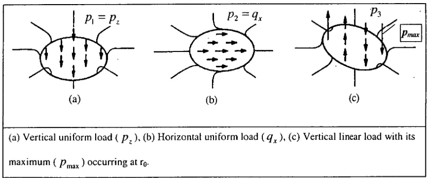
Figure 2.3 Cylindrical coordinates and an infinitesimal circular loaded area (radius r0) 35 Figure 2.4 Illustration of load cases considered by Gerrard and Wardle (1973) 35 Figure 2.5 Stress resolution for the load cases considered in this study (Gerrard and

Harrison 1970a) 38

Figure 2.6 Variation of shear modulus in an inhomogeneous soil idealised by Gibson

(1967) 42

Figure 3.1 Coordinate systems, superstructure, soil medium and the interaction 52 Figure 3.2 Illustration of soil and superstructure nodal reactions at the interface 55 Figure 3.3 Illustration of different sub-matrix groups in soil flexibility between two

points 56

Figure 3.4 Orientation of direction vector for point P (i, j, k) 57 Figure 3.5 Flexibility coefficients associated with the horizontal and vertical degrees of

freedom at point b due to horizontal force Qa at point a 57

Figure 3.6 Illustration of flexibility coefficients in soil flexibility matrix [f]ab 58 Figure 3.7 Profile of the surface displacement components due to horizontal surface force

Qb 60

Figure 3.8 Equivalent situations in flexibility coefficients due to symmetry in the soil

flexibility matrix 60

Figure 3.9 Resolution of moment Ma into a vertical couple acting on the surface of the

medium 60

Figure 3.10 Profile of the surface horizontal and vertical displacements due to vertical

force ( Pb ) 61

Figure 3.11 Rotations 0a and 0, due to the vertical point load Pb 62

Figure 3.12 Replacement of moment _Mb with a couple, and the vertical displacement 63

Figure 3.13 Total zero vertical displacement due to horizontal load Qb 65 Figure 3.14 Load distribution over a circle on the soil replacing moment Mb 69

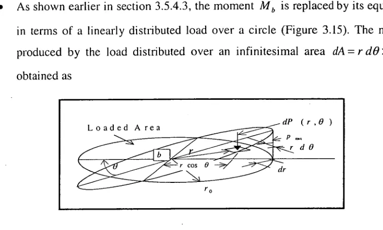
Figure 3.15 Load distribution over a circle on the soil replacing moment Mb 78

Figure 4.1 Overview of SASIAP analysis package 82

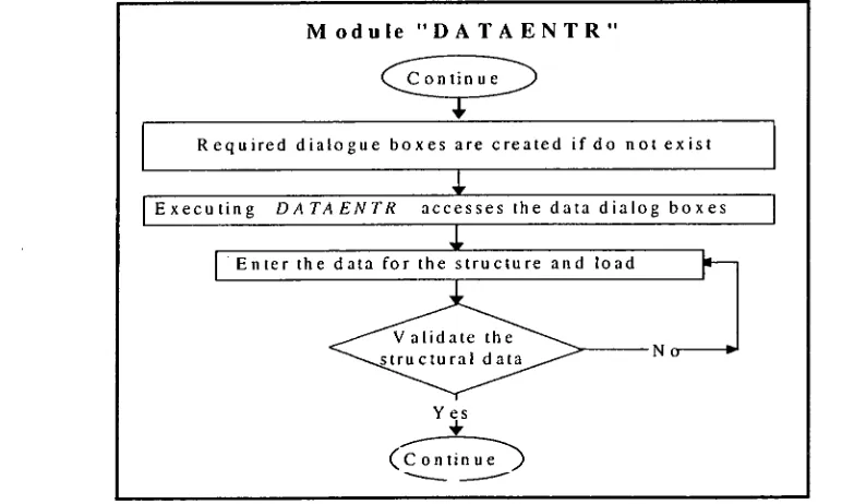
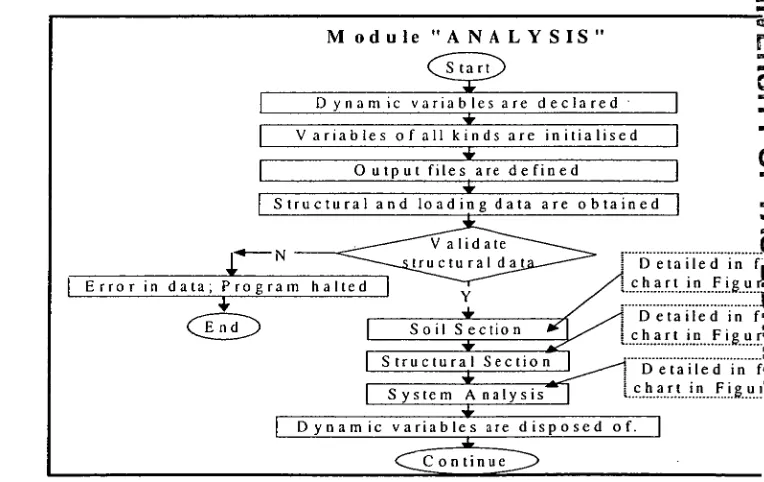
Figure 4.2 Flow chart for module "DATAENTR" 83 Figure 4.3 Flow chart for module "ANALYSIS" 84 Figure 4.4 Flow chart for soil section in the soil-structure analysis 85 Figure 4.5 Flow chart for structure consideration in analysis procedure 86

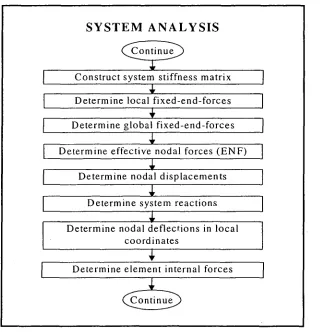
Figure 4.6 Flow chart for the system analysis 86

Figure 5.1 Illustration of a single plane frame considered for two cases: (a) No interactive

support, and (b) With interactive support 89

(14)

Figure 5.5 Nomination of symbols to element end-node moments associated with plane

frame resulting from structural analysis 93

Figure 5.6 Nomination of symbols to nodal displacements associated with analysis 94 Figure 6.1 Illustration of parameters hierarchy in system analysis 148

Figure A1.1 Parameters used for a distributed load over a circle 1-1 Figure A1.2 Surface vertical displacement due to a uniformly loaded rectangular area on

elastic half space (Cheung and Zienkiewicz 1965) 1-2 Figure A2.1 Illustration of the Mindlin's case in x-z plane within the medium 2-1 Figure A2.2 Stress definitions in triaxial test 2-15 Figure A3.1 Element free-body diagram in local coordinates 3-1 Figure A3.2 Stiffness matrix for a structure with two members and three nodes 3-3 Figure A3.3 Orientation of displacements and forces in both coordinate systems 3-3 Figure A3.4 Orientation of fixed-end forces in the local coordinates 3-5 Figure A4.1 Illustrates the introduction of DataEntr program 4-2 Figure A4.2 A blank text associated with a default title 4-3 Figure A4.3 The Data menu bar and its pull-down items 4-3 Figure A4.4 Accessing and opening an existing structure data file 4-3 Figure A4.5 Illustration of window Save As to save a file under a name other than the

original 4-3

Figure A4.6 Illustrates the root and current directories for any new location of a directory 4-4

Figure A4.7 DOS shell access within the program 4-4

Figure A4.8 Illustrates the items on the Edit data pull-down menu 4-5 Figure A4.9 Window associated with the title of a structure 4-5 Figure A4.10 Selection of a data file associated with Geometry of Structure nodes 4-6 Figure A4.11 Geometry details of a structure node entered or edited 4-6 Figure A4.12 Window to access a file of material properties 4-6 Figure A4.13 Illustration of material properties data window 4-6

Figure A4.14 Allocating a cross section data file 4-7

Figure A4.15 Cross-section properties associated with structure members 4-7

Figure A4.16 Allocating a member data file 4-7

Figure A4.17 Data associated with members of a structure 4-7

Figure A4.18 Allocating a file for Restraint data 4-8

Figure A4.19 Information associated with node restraints 4-8

Figure A4.20 Load pull-down menu 4-8

Figure A4.21 Allocating Prescribed Load file 4-9

Figure A4.22 Details of prescribed displacement loads applicable to structure nodes 4-9

Figure A4.23 Allocating Node load file 4-9

Figure A4.24 Details of Node loads applicable to structure 4-9 Figure A4.25 Allocating file associated with member concentrated load 4-10

Figure A4.26 Details of member concentrated load 4-10

(15)

LISTING OF TABLES

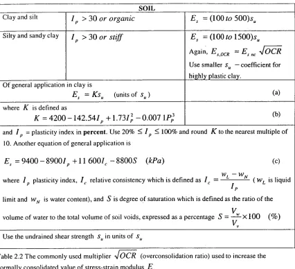
Table 2.1 Equations defining stress-strain modulus Es by several test methods 45

Table 2.2 The most commonly used multiplier VOCR (overconsolidation ratio) used

to increase the normally consolidated value of stress-strain modulus Es,n, 46

Table 2.3 Values and some value ranges for Poisson's ratio ki for selected materials 46

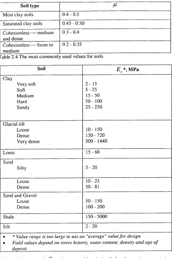
Table 2.4 The most commonly used values for soils 47

Table 2.5 A range of Es values (possibly obtained) for the static stress-strain modulus

Es for selected soils 47

Table 5.1 Table of soil elastic properties considered in this research 95 Table 5.1a Isotropic elastic soil constants (Gerrard 1967) 96 Table 5. lb Table of properties for cross-anisotropic soil Gerrard (1967) 97 Table 5.1c Listing of elastic properties for Isotropic and Cross-anisotropic soil sub-cases

32-36 (Wardle 1977) 98

Table 5.1d Listing of elastic properties for Isotropic soil sub-cases 37, 39, 40 and its

equivalent of Winkler spring 98

Table 5.2 Output data for element bending moment M21 from structure analysis when

soil modulus of elasticity (Young's modulus ) varies between 5 and 150

MPa for three different interaction cases 99

Table 5.3 Element end moments 117

Table 5.4. Nodal displacements in x and y directions are in meters, and rotation in z

direction is in radian 117

Table 5.5 Support reactions in x and y directions are in kN, and for z direction is in

kN.m 117

Table 5 6 Bending moment M 21 for different Winkler springs and corresponding

Isotropic values 118

Table 5.7 Bending moment M32 for different Winkler springs and corresponding

Table 5.8 Bending moment M34 for different Winkler springs and corresponding

Table 5.9 Nodal displacement A different Winkler springs and corresponding

Table 5.10 Nodal displacement A y, for different Winkler springs and corresponding

Table 5.11 Nodal rotation 0,1 for different Winkler springs and corresponding Isotropic

values 119

Table 5.12 Nodal displacement A3 for different Winkler springs and corresponding

Table 5.13 Nodal displacement A 3 for different Winkler springs and corresponding

Table 5.14 Nodal rotation 0,3 for different Winkler springs and corresponding Isotropic

values 120

Table 5.15 Nodal reactions from interaction analysis (Isotropic El, = 50 MPa,

v = 0.25 ) 122

Table 5.16 Members end moments (kN.m) from interaction analysis (Isotropic

(16)

Table 5.17 Nodal displacements (m ) Angle of rotation (rad) from interaction analysis

(Isotropic E,.= 50 MPa, V =0.25) 122

Table 5.18 Verification of displacements for sample: 7-1Iso D 123 Table 5.19 Verification of displacements for sample: 7-1Iso P 124 Table 5.20 Verification of displacements for sample: 7-1Iso S 125

Table 5.21 Bending moment ( M21) vs Isotropic soil modulus of elasticity EH for V =

0.25 127

Table 5.22 Bending moment ( M32 ) vs Isotropic soil modulus of elasticity EH for V =

0.25 127

Table 5.23 Bending moment ( M34) vs Isotropic soil modulus of elasticity EH for V =

0.25 127

Table 6.1 Variation of bending moments M21, M32, M34 for Es =20 MPa, and

corresponding items (V0.25 - v043) in percentage 131 Table 6.2 Variation of bending moments M,1 , M32, M34 for Es =50 MPa, and

corresponding items (Tables 6.2 - Table 6.1) in percentage 131

Table 6.3 Variation of bending moments M21, M32, M34 for Es =70 MPa, and

Table 6.4 Variation of nodal displacements/rotation 6,„1, Ay!, (13,1 for Es =20 MPa, and

corresponding items (v0.25 - V0.43 ) in percentage 132 Table 6.5 Variation of nodal displacements/rotation Axi,i, 13,[ for Es =50 MPa, and

Table 6.6 Variation of nodal displacements/rotation Axi, Ayi, cla,1 for Es =70 MPa, and

Table 6.7 Variation of nodal displacements/rotation 6,0, Ay3, cI)z3 for Es =20 MJ'a, and

corresponding items (v0.25 - v043) in percentage 133 Table 6.8 Variation of nodal displacements/rotation Ax3, Ay3, C13,3 for Es =50 MPa, and

Table 6.9 Variation of nodal displacements/rotation Ax3, Ay3, Ci3x3 for Es =70 NIPa, and corresponding items (Tables 6.9 - Table 6.7) in percentage 133

Table 6.10 Variation of bending moments M21 , M32, M34 for- Ev-26 MPa and Ev=35 MPa in a soft to medium soil, corresponding (Ev35 - Ev26) in

percentage 138

Table 6.11 Variation of bending moments M21 , M32, M34 for Ev=75 MPa and Ev=84 MPa in a medium to hard soil, corresponding (Table 6.11 - Table

6.10) in percentage 138 Table 6.12 Nodal displacements/rotation kb cIolz, for Es=26 MPa, and 35 MPa in a

soft to medium soil, corresponding (Ev35 - Ev26) in percentage 139 Table 6.13 Nodal displacements/rotation A„,, i,crozi for Es=75 MPa, and 841VIPa in a

medium to hard soil, corresponding (Table 6.13 - Table 6.12) in percentage 139 Table 6.14 Nodal displacements/rotation Ax3, Ay,3, 413,3 for Es=26 MPa, and 35 MPa in a

soft to medium soil, corresponding (Ev35 - Ev26) in percentage 140 Table 6.15 Nodal displacements/rotation 6,,3, Ay3, (1)z3 for Es=75 MPa, and 84 MPa in a

medium to hard soil, corresponding (Table 6.15 - Table 6.14) in percentage 140

Table 6.16 Variation of bending moments M21 , M32, M34 versus soil shear modulus

of elasticity Fv 142

Table 6.17 Variation of nodal displacements/rotation Axi, Ayl, cI3z, versus soil shear

modulus of elasticity Fv 142

Table 6.18 Variation of nodal displacements/rotation 6,„3, Ay3, (I3z3 versus soil shear

(17)

Table A2.1 Presumptive values of CBR for different types of soil (Austroads, Pavement

and Design 1992) 2-16

Table A5.1 Bending moment M21 vs Isotropic soil modulus of elasticity EH for v=0.25 5-1 Table A.5.2 Bending moment M32 VS Isotropic soil modulus of elasticity EH for v=0.25 5-1 Table A5.3 Bending moment M34 vs Isotropic soil modulus of elasticity EH for v=0.25 5-1 Table A5.4. Nodal displacement (Axi ) vs soil modulus of elasticity (E H) Isotropic v = 0.25 5-2 Table A5.5 Nodal displacement (Ayi ) vs soil modulus of elasticity (E H) Isotropic v = 0.25 5-2 Table A5.6 Nodal rotation (0, 1 ) vs soil modulus of elasticity (EH) Isotropic v= 0.25 5-2 Table A5.7. Nodal displacement (A,3 ) vs soil modulus of elasticity (E H) Isotropic v -= 0.25 5-3 Table A5.8 Nodal displacement (Ay3) vs soil modulus of elasticity (E H) Isotropic v = 0.25 5-3 Table A5.9 Nodal rotation (0,3) vs soil modulus of elasticity (E H) Isotropic v = 0.25 5-3 Table A5.10 Bending moment (M 21 ) vs soil modulus of elasticity (E H) Isotropic v = 0.43 5-4 Table A5.1 I Bending moment (M 32) vs soil modulus of elasticity (E H) Isotropic v = 0.43 5-4 Table A5.12 Bending moment (M 34) vs soil modulus of elasticity (E H) Isotropic v = 0.43 5-4 Table A5.13 Nodal displacement (A, 1 ) vs soil modulus of elasticity (E H) Isotropic v = 0.43 5-5 Table A5.14 Nodal displacement (Ay ) vs soil modulus of elasticity (EH) Isotropic v = 0.43 5-5 Table A5.15 Nodal rotation (0, 1 ) vs soil modulus of elasticity (E H) Isotropic v= 0.43 5-5 Table A5.16 Nodal displacement (A,(3 ) vs soil modulus of elasticity (E H) Isotropic v = 0.43 5-6 Table A5.17 Nodal displacement (4, 3) vs soil modulus of elasticity (E H) Isotropic v = 0.43 5-6 Table A.5.18 Nodal rotation (0,3) vs soil modulus of elasticity (E H) Isotropic v = 0.43 5-6 Table A5.19 Bending moment (M 21 ) vs soil modulus of elasticity of cross-anisotropic soil

Ev 5-7

Table A5.20 Bending moment (M 32) vs soil modulus of elasticity of cross-anisotropic soil

Ev 5-7

Table A5.21 Bending moment (M34) vs soil modulus of elasticity of cross-anisotropic soil

Ev 5-7

Table A5.22 Nodal displacement (A xi ) vs soil modulus of elasticity of cross-anisotropic

soil Ev 5-8

Table A5.23 Nodal displacement (Ayi ) vs soil modulus of elasticity of cross-anisotropic

soil Ev 5-8

Table A5.24 Nodal rotation (0, 1 ) vs soil modulus of elasticity of cross-anisotropic soil Ev 5-8 Table A5.25 Nodal displacement (A, 3) vs soil modulus of elasticity of cross-anisotropic

soil Ev 5-9

Table A5.26 Nodal displacement (A y3) vs soil modulus of elasticity of cross-anisotropic

soil Ev 5-9

Table A5.27 Nodal rotation (:13 z3) vs soil modulus of elasticity of cross-anisotropic soil Ev 5-9 Table A5.28 Bending moment (M21 ) vs soil modulus of elasticity of cross-anisotropic soil

Ev 5-10

Table A5.31 Nodal displacement (A, 1 ) vs soil modulus of elasticity of cross-anisotropic

soil Ev 5-11

Table A5.32 Nodal displacement (A y1 ) vs soil modulus of elasticity of cross-anisotropic

soil Ev 5-11

Table A5.33 Nodal rotation (4:13, 1 ) vs soil modulus of elasticity of cross-anisotropic soil Ev 5-11 Table A5.34 Nodal displacement (A x3) vs soil modulus of elasticity of cross-anisotropic

soil Ev 5-12

Table A5.35 Nodal displacement (A y3 ) vs soil modulus of elasticity of cross-anisotropic

soil Ev 5-12

Table A5.36 Nodal rotation (313,3) vs soil modulus of elasticity of cross-anisotropic soil Ev 5-12 Table A5.37 Bending moment (M21 ) vs soil modulus of elasticity of cross-anisotropic soil

Fv 5-13

(18)

Table A5.40 Nodal displacement (A,(1) vs soil modulus of elasticity of cross-anisotropic

soil Fv 5-14

Table A5.41 Nodal displacement (Ayi) vs soil modulus of elasticity of cross-anisotropic

soil FN./ 5-14

Table A5.42 Nodal rotation (cDzI) vs soil modulus of elasticity of cross-anisotropic soil Fv 5-14 Table A5.43 Nodal displacement (Ax3) vs soil modulus of elasticity of cross-anisotropic

soil Fv 5-15

Table A5.44 Nodal displacement (6,0) vs soil modulus of elasticity of cross-anisotropic

soil Fv 5-15

(19)

LISTING OF GRAPHS

Graph 5.1 Bending moment (M21) vs soil modulus of elasticity (EH) Isotropic v = 0.25 100

Graph 5.3 Bending moment (M34) vs soil modulus of elasticity (E11) Isotropic v = 0.25 100

Graph 5.4 Nodal displacement (Ad) vs soil modulus of elasticity (EH) Isotropic v = 0.25 101

Graph 5.5 Nodal displacement (Ad ) vs soil modulus of elasticity (EH) Isotropic v = 0.25 101

Graph 5.6 Nodal rotation (43,1) vs soil modulus of elasticity (EH) Isotropic v = 0.25 101

Graph 5.7 Nodal displacement (Ax3) vs soil modulus of elasticity (EH) Isotropic v = 0.25 102

Graph 5.8 Nodal displacement (Ay3) vs soil modulus of elasticity (EH) Isotropic v = 0.25 102

Graph 5.1 I Bending moment (M32) vs soil modulus of elasticity (EH) Isotropic v = 0.43 103

Graph 5.13 Nodal displacement (Ad) vs soil modulus of elasticity (EH) Isotropic v = 0.43 104

Graph 5.14 Nodal displacement (A) ) vs soil modulus of elasticity (EH) Isotropic v = 0.43 104

Graph 5.16 Nodal displacement (A,3) vs soil modulus of elasticity (EH) Isotropic v = 0.43 105

Graph 5.17 Nodal displacement (Ay3) vs soil modulus of elasticity (EH) Isotropic v = 0.43 105

Graph 5.18 Nodal rotation (0,3) vs soil modulus of elasticity (EH) Isotropic v =0.43 105

Graph 5.19 Bending moment (M21) vs soil modulus of elasticity of cross-anisotropic soil

Ev 107

Graph 5.22 Nodal displacement (Ax1) vs soil modulus of elasticity of cross-anisotropic soil

Ev 108

Graph 5.23 Nodal displacement (Ay1) vs soil modulus of elasticity of cross-anisotropic soil

Ev 108

Graph 5.24 Nodal rotation (elpd) vs soil modulus of elasticity of cross-anisotropic soil Ev 108

Graph 5.25 Nodal displacement (A,3) vs soil modulus of elasticity of cross-anisotropic soil

Ev 109

Graph 5.27 Nodal rotation (0,3) vs soil modulus of elasticity of cross-anisotropic soil Ev 109

Ev 110

Graph 5.31 Nodal displacement (Ad) vs soil modulus of elasticity of cross-anisotropic soil

Ev 111

Graph 5.34 Nodal displacement (A,3) vs soil modulus of elasticity of cross-anisotropic soil

Ev 112

(20)

Graph 5.38 Bending moment (M32) VS soil modulus of elasticity of cross-anisotropic soil

Fv 114

Graph 5.40 Nodal displacement (A„,) vs soil modulus of elasticity of cross-anisotropic soil

Fv 115

Nodal rotation (49,1) vs soil modulus of elasticity of cross-anisotropic soil Fv 115 Nodal displacement (6,0) vs soil modulus of elasticity of cross-anisotropic soil

Fv 116

Nodal displacement (Ay3) VS soil modulus of elasticity of cross-anisotropic soil

Fv 116

Nodal rotation (0,3) vs soil modulus of elasticity of cross-anisotropic soil Fv 116

Verification of results for bending moment ( M21 ) VS soil modulus of elasticity

(EH) Isotropic V = 0.25 126

Verification of results for bending moment ( M₃₂) VS SOH modulus of elasticity

126

Verification of results for bending moment ( M 34 ) VS Soil modulus of elasticity

(EH) Isotropic V = 0.25 126

Correlation of static cone penetrometer and CBR (Pavement Design 1992) 2-12 Correlation of dynamic cone penetrometer and CBR (Pavement Design 1992) 2-13 Variation in stiffness parameters used in equation (2.79) with load repetitions

(Barret and Smith (1976) ) 2-15

Graph 5.42 Graph 5.43

Graph 5.44

Graph 5.45 Graph 5.46

Graph 5.47

Graph 5.48

Graph A2.1 Graph A2.2 Graph A2.3

(21)

CHAPTER

ONE

INTRODUCTION

(22)

ELASTOSTATIC INTERACTION ANALYSIS OF FRAMES RESTING ON HOMOGENOUS ELASTIC HALF-SPACE

Chapter 1 Introduction

Chapter 2 Soil Idealisation

Chapter 3 Method of Solution

Chapter 4 Software Development

Chapter 5

Examples of Analysis Applications Chapter 6

Discussion of Results Chapter 7

Summary and Conclusions

CHAPTER 1 INTRODUCTION

1.1. THESIS OUTLINE

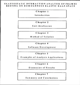
[image:22.559.158.435.414.709.2]

The study described in this thesis focuses on the analysis of the interaction of elastostatic linear plane frame structures and their supporting media modeled as homogeneous elastic half-space with isotropic and cross-anisotropic properties. In the isotropic soil idealisation, Boussinesq's solutions (1885) are utilised for the application of vertical point load to the surface of elastic half-space, and Cerruti's solutions (1882) are used for the horizontal loads. The analysis is enhanced by a well-known force-displacement analytical method, termed the Direct Stiffness Method (DSM). For the case of cross-anisotropic media, the solutions of Gerrard and Harrison (1970a) and Gerrard and Wardle (1973) have been implemented to express the force-displacement relationship. These models are described in detail in the next chapter. Figure 1.1 shows a flow chart of the thesis chapters and their organisation.

(23)

Chapter 1, is an introductory section, which establishes the context of soil-structure interaction. The importance of the soil characteristics in the analysis is described and a summary of past work is outlined in a literature review. Different soil models are reviewed, and their important parameters are identified. The chapter concludes with a description of possible benefits that may result from the project.

Chapter 2 outlines the general idealisation of the superstructure and soil models in use (sections 2.3.2 and 2.4). The soil is represented by a half-space medium with isotropic and cross-anisotropic properties.

Chapter 3 establishes the descriptive matrices for the soil and the superstructure using the proposed analytical/ numerical models.

Chapter 4 describes the different processes and procedures that were developed and used in each step via their corresponding flow charts. These were constituted into an integrated computer package (SASIAP) that facilitates the analysis of soil-structure interaction for different applications. The package enables the user to extend the application of the models that were utilised for a plane frame analysis, to the third dimension for analysing the interaction caused by the neighbouring frames. The total assemble then constitutes a space frame.

Chapter 5 presents a number of soil-structure examples using different soil models. In these examples, superstructures with different support conditions are considered, and typical results obtained are tabulated for discussion in chapter 6.

In chapter 6 a discussion of the model output is carried out, and some conclusions are presented on the effects of the various parameters on model output.

(24)

1.2. STATE OF THE ART: SOIL-STRUCTURE INTERACTION

In the early years of investigating soil-structure interaction, the analyses of the structure and that of the soil were undertaken independently. In such an approach, the structural responses within a building were calculated on the assumption that the footings of the structure were rigid. The resulting reaction forces at the supports were then used by soil mechanics specialists to calculate foundation settlements based on a completely flexible structure. However, with more research in this field, new methods of analyses were developed that form the basis of a more rational approach to foundation design that integrates soil and structure (Lee & Harrison 1970; Goschy

1978; Desai et al. 1982; Masih 1985, 1993).

At present, it is widely recognised that the response of a structure is strongly dependent upon the behaviour of the soil underneath. Due to different soil support conditions, the structure can undergo various deflections in response to its external loads. These deflections are associated with soil deformation, which has two components: the short term elastic component, and the long term (or permanent) plastic (consolidation) component. This research focuses on the elastic solutions for the soil deformation.

To consider the nature of loads applied to the soil, there are two major types: static and dynamic. The response of the soil structure and the interaction of the soil and the structure vary greatly with load type. A study of all load types is beyond the scope of this thesis and only static loads are considered.

(25)

elasticity. Numerous refinements are possible depending upon the soil type, which can be classified as an environment with elastic, elasto-plastic, visco-elastic or even critical state material with time-dependent properties.

The degree of cohesion and density of soil determines the responses of the supporting medium with respect to the interaction (Masih 1985). Existence of water and its quantity are other important issues that designers are required to be aware of as all engineers recognise that the presence of water can greatly alter the performance or response characteristics of the soil.

1.3. SIGNIFICANCE OF SOIL CONSIDERATION

The analysis of the interaction between a structure's foundation and the supporting soil medium is of great importance to structural and geotechnical engineering. Theoretical results can provide information that can be used in both foundation and structural design. The quality of soil is important in structural design as it affects the size of the members as well as the foundation of the structure, and hence influences the economy of the structure.

The amount of research work carried out in the past, and the broad present interest in this field testify to the significance of soil characteristics in soil-structure interaction analysis. This interest has also motivated the extension of. investigations into different aspects of the soil-structure interaction.

One aspect of soil characteristics is its behaviour due to external dynamic loads. Seed et al. (1975) studied dynamic soil-structure interaction with respect to the seismic design of nuclear power plants and pump stations. These researchers emphasised the significance of soil in prediction performance and the requirement for some design procedures to increase the validity of analysis techniques. Furthermore, they concluded that uncertainties in determining soil properties give rise to difficulties in accurately evaluating the characteristics of ground movements.

(26)

foundations. They pointed out that the static response between the footings is different from that of the dynamic case. The result of the interaction in the static case may fall in an expected range. However, in the dynamic case the material properties of soil, when included in the analysis, require some alteration to accurately predict field performance.

Dieterman and Metrikine (1996) studied the dynamic properties of isotropic elastic half-space medium. Later, Metrikine and Dieterman (1997) proposed equivalent vertical stiffness for such a medium interacting with a beam taking into account the shear stress acting in the beam.

More recently, Gazetas and Mylonakis (1998) considered a variety of soil models to evaluate the soil-structure interaction. Furthermore, in the study by Stewart et al. (1999a), the analytical procedures and system identification techniques for evaluating the inertial soil-structure interaction effects on a seismic structural response were discussed. A collective examination of the empirical and predicted results from a number of sites revealed a pronounced influence of structure-to-soil stiffness ratio on inertial interaction, as well as secondary influences from the structure aspect ratio and the foundation embedment, type, shape and flexibility (Stewart et al. 1999b).

To express the significance of the "static" interaction of soil and structure, Meyerhof (1947), Francis (1954) and Chamecki (1956) developed interaction analyses for multi-storey multi-bay structures on isolated frames. These analyses were superseded by Lee's method (Lee 1969), which required only minor amendments to those previous analysis procedures. This method was named "the fictitious member technique", where the supporting soil was replaced by a small structural member at each column base where its axial stiffness was considered equal to the relevant stiffness of the footing-supporting soil at each column. Lee (1975) emphasised the analysis of structure based on the above technique, and considered the interaction for the major types of foundations, namely, isolated footings, piles and rafts.

(27)

effect of differential displacements of column bases and the internal forces was presented, and he investigated the important factors that control the magnitude of the interaction. In his findings, several factors such as the combination of relative stiffness at which reduction in differential displacement occurs, increase in column stiffness, the number of storeys and the thickness of the beam foundation, can possible decide when full interaction effects are of little significance and a complete analysis can be avoided.

For an economical design of a structure, it is important to consider the soil as part of the medium that is exposed to the external loads. In such a design, it is essential to study the loads transmitted to the soil and the resulting stress distributions within the soil itself. The study of the physical state of foundation materials, and overall foundation plan and design, are important in avoiding any excess settlement or soil failure. A complete interaction analysis should involve the following:

a) The distribution and intensity of pressure between the footing and the foundation medium (contact pressure)

b) The intensity of normal and shearing stresses at various points within the mass of the medium

c) Any possible mechanism of soil failure underneath the foundation after considering the soil's physical characteristics as found by initial soil tests.

Over the years, various computer packages have been developed that idealise soil using finite elements and employ various assumptions. Some methods need more input data for their parameters than other approaches. In the later sections of this chapter, a review of the process of development of soil models and methods is presented.

1.4. LITERATURE REVIEW

(28)

PLASTIC

VISCOUS ! ; MULTIPIIASE • STATISTICAL ! ; HALF-SPACE THEORY

NON • HOMOGENEOUS (HETEROGENEOUS)

D ISC R ETE (D ISCONTIN UUM )

_.;

NON LINEAR

HOMOGENEOUS

LI A LT.-SPA C E RE FIN ENTS'0

ELASTIC •

Ai 0 G E E0_{. .}us

ISOTROPIC A N ISOTROPIC

(cross.:anisotropic) c,c)

NT IN U'O.0 S D.IS CO N T IN U•,0 U S IN G LE.-

PAR A M'EtER.•

;

C ON TIN U U M

NO PI- • H'0 M.,0.6 E NE GU S , (H,E T Eli 0 d'•E NE GUS) '

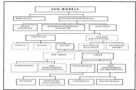
• , With static interaction analyses, there are three major categories for soil models: • Infinitely rigid,

• Elastic, which includes single-parameter, modified single-parameter,

homogeneous isotropic half-space, homogeneous cross-anisotropic half-space and non-homogeneous half-space,

• Visco-elastic/ plastic media which is not the focus of this research.

Solutions to express soil behaviour based on the assumption of a continuum can be grouped according to the classification of the half-space in question. Stress calculations can be classified from a mathematical point of view, that is, whether they lead to a closed form (for example elastic half-space) or an open form (numerical methods, for example Finite Element Method (FEM)) solution. In Figure

1.2, the shaded models are the soil idealisations that are considered in this project.

SO IL M 0 D EL,S

[image:28.559.76.521.316.611.2]

RIGID MODEL S T le / PLASTIC 'M Ei ELS

Figure 1.2 Classification of soil models and methods of stress consideration and calculation.

(29)

to introduce new and improved soil models. However, these models often appeared to have some shortcomings. To rectify these deficiencies, successive investigators defined extra parameters in their idealisations as refinements to earlier models. Examples are flexural rigidity (D) and tension field (T).

As a result of later efforts in adopting a soil model, a homogeneous isotropic elastic continuum (the soil parameters are Young's modulus and Poisson's ratio) was identified. In addition, for a more complex case (for example a layered soil), a homogeneous cross-anisotropic half-space was defined in which five independent parameters are used to describe the medium.

The majority of the existing solutions using analytical or numerical techniques for isotropic or cross-anisotropic homogeneous half-space are in general tedious to utilise. With these approaches, solutions often involve differential equations of high order, which produce many answers. In these cases it is required to implement the boundary conditions to confirm acceptable results, and to simultaneously eliminate the general answers to those differential equations.

Poulos (1975a) analysed settlement of structure-foundation systems considering relative structural stiffness. Davis and Poulos (1968) and Poulos (1975b) summarised some of the more commonly used methods [such as the Conventional One-dimensional method, Skempton and Bjemim's (1957) method, the Effective Stress Path method, the Elastic method, Cambridge approach and Finite Element Method (1-EM)], to calculate the settlement of isolated foundations.

(30)

confirmed the application of operational stiffness for evaluation of settlements in non-cohesive soils.

Cheung and Zienkiewicz (1965) found that the Winkler type spring approximation introduced to avoid mathematical difficulties need no longer be used where continuous foundations are present, and no special treatment of holes, corners or other irregularities in the foundation plate was necessary (refer to Appendix Al). Therefore, practical cases such as variable thickness foundation rafts or other shapes of foundations were capable of rapid solution. More recently Montrasio and Nova (1997) studied the effect of shape of foundation on the settlement of shallow foundations where they employed a number of mathematical methods. They found that experimental evidence is generally well matched by theory of elasticity. It was shown that only two out of nine parameters that characterised their model varied significantly with the shape of the foundation. They concluded that embedment has a small influence on the value of additional two parameters and the other five remain constant.

There are several soil models used in soil-structure interaction analysis and some of these are briefly reviewed in this chapter. This study however, focuses on soil medium with linear homogenous isotropic and cross-anisotropic properties. For the former, the solutions of Boussinesq (1885), Cerruti (1882) and Mindlin (1936) have been used and for the latter, those presented by Gerrard and Harrison (1970a) and Gerrard and Wardle (1973) have been implemented. Of these approaches, Mindlin's solution applies to the interior of the half-space while the remaining approaches are applicable to the surface of the medium.

1.4.1. Rigid Model

(31)

practice imply, any foundation displacement affects the internal forces of the superstructure. Therefore, this early idealisation of soil was unrealistic and encouraged research into utilising the elastic behaviour of soil in the structural analyses of the building.

1.4.2. Winkler Model and Its Applications

The Winkler springs or Winkler model (1867) was the first elastic idealisation of soil. According to this theory, soil is assumed to be a series of independent springs, all with a constant stiffness, that react against vertical forces transferred from the structure. These vertical reaction forces are considered directly proportional to the local vertical displacement of the foundation. This model is a single-parameter soil idealisation used to describe the stresses produced in the soil beneath the foundation. The relationship is defined by a parameter

(lc)

known as the modulus of sub-grade reaction, and for a beam resting on a medium idealised by such a model (two-dimensional application) the stress is given by

p(x) = w(x) (1.1a)

where k, is the modulus of foundation or sub-grade reaction, with its dimension being in pressure per length of vertical displacement in the range of 5 - 50 MN I m3.

The function w(x) is the vertical deflection (i.e. z direction, perpendicular to the beam) beneath the foundation (Figure 1.3).

The general form of the Winkler model in a three-dimensional application (a plate in

x— y plane) is described as

p(x, y) = w(x, y) (1.1b)

where p(x, y) is the intensity of reaction of the soil, and w(x, y) is vertical deflection (in the z direction, perpendicular to the plate) beneath the foundation.

(32)

A plate

(Three-dimension problem)

a) Presentation of Winkler model b) Observed displacement

under uniform load under uniform load

Figure 1.3 Illustration of sign convention for a beam and a plate foundation resting on Winkler model.

Figure 1.4 Illustration of soil deformations: (a) under external load for Winkler model, and (b) the

observed deflections on site in the real situation.

From Figure 1.4a, it can be observed that in a Winkler medium, the displacement under the loaded area is constant when it is subjected to a uniform external load, whilst the displacement outside the loaded zone is zero. The observed field behaviour of soil under a uniform load is as shown in Figure 1.4b. This difference between the behaviour of the real soil and that of a Winkler soil is one of the major shortcomings of the Winkler model. For this reason, several researchers have suggested refinements to the Winkler model to improve its application as a soil idealisation.

(33)

use there are some inherent disadvantages. As indicated earlier, it is the lack of continuity in the supporting medium in the model that is physically unrealistic.

Many researchers, (Lee and Brown 1972 and Selvadurai 1979) addressed the model's limitations and inherent difficulties in solving soil-structure interaction problems using various continuum models. Vlasov and Leontiev (1966) attempted to overcome the shortcomings of the model by incorporating foundation flexural rigidity as a second parameter in soil idealisation for the analysis of a rigid circular foundation under both uniform and non-uniform vertical load.

Schleicher (1926) and Conway (1955) studied the axi-symmetrical loading of a circular foundation using the Winkler model, and Hetenyi (1946 and 1950) suggested an interaction between independent spring elements and a beam (2D problem) or plate (3D problem), assuming bending in the beam or plate.

The Winkler model was further investigated and developed using different methods of analysis and different numerical techniques for the analysis. A number of researchers in the past, Lee and Brown (1972), Selvadurai (1979), and more recently, Melerski (1992, 1995a, 1995b) used finite element and finite difference techniques in analysing soil-structure interaction via Winkler springs.

As indicated earlier, the Winkler model is a single-parameter soil idealisation. Over the years, extra parameters such as tension field or shear interactions between the spring elements, and flexural rigidity for foundation plate were incorporated into the analysis to rectify the shortcomings of this soil model (Filonenko-Borodich 1940, Hetenyi 1946 and Pasternak 1954). Further discussion on Winkler refinements can be found in Kerr (1964).

(34)

plate in frictionless and continuous contact with a homogenous half-space. The significance of the homogeneous half-space model is discussed in the next section.

1.4.3. Homogeneous Isotropic Elastic Half-space Model

One of the frequently used models for soil idealisation is a homogeneous isotropic elastic half-space. There are two parameters that are utilised in this model, modulus of elasticity (E), and Poisson's ratio ( v ). The first parameter associates the deformation in the soil and the stresses applied to it when these are in the same direction. Vertical deformation in the medium is related to the stress applied to the medium in the horizontal direction and vice versa. This relationship is expressed by Poisson's ratio.

Boussinesq (1885) proposed soil to be an elastic homogeneous half-space medium of isotropic material. He solved the problem of a vertical point load acting on the surface of the medium and gave solutions for the stresses and displacements at any point in the medium. For similar media Cerruti (1882), analysed the problem of a horizontal point load acting on the surface and developed solutions for the stresses and displacements at any point within the medium. The above two researchers were at the frontier in solving the problems of elastic isotropic half-space at that time.

Based on the fundamental results from the theory of elasticity known as the Kelvin solution (1848), further studies were undertaken by Love (1927) and Timoshenko (1934). Solutions to the problem of stress distribution for a number of cases have been obtained using the Kelvin solution.

For application of loads within a homogenous elastic half-space, Melan (1932) developed solutions to evaluate stresses and strains for a two-dimensional application. Mindlin (1936) provided similar expressions for a three-dimensional application. These expressions were similar in nature to Boussinesq's and Cerruti's findings for surface loads.

(35)

moment on an elastic half-space. Lee and Brown (1972) performed a comparative analysis of the structure-foundation interaction between Winkler's model and linear elastic models in the form of the Boussinesq model.

In further studies, Hain and Lee (1980) examined the influence of interaction between a 3D structure and its footing founded on isotropic elastic half-space. They concluded that the interaction behaviour of a three-dimensional frame and a raft foundation can be predicted if the relative stiffness of structures (Ks) to the rafts

(KR) is in the range: 0.1 <K I KR < 10.0 then redistribution of column loads largely occurs. They also found that an increase in differential settlements, maximum negative bending moment, and reduction in maximum positive bending moment occur. This is due to increased interaction caused by an increase in the number of bays in the structure.

In the past few years, there have been a number of studies undertaken by several researchers in relation with soil-structure interaction. Huang and Tatsuoka (1988), Khing et al. (1992) and Takemura et al. (1992) considered improvements for analysing and predicting behaviour for footings placed in sandy ground. Delgado and Faria (1994) investigated soil-structure interaction for dam-foundation-reservoir interaction to obtain assurance of dam safety and performance due to earthquakes. In this work numerical modeling aspects of foundations were described.

Huang and Meng (1997) analysed deep footing and width effects in the elastic half-space medium by considering the results of 105 models tested in their investigation. More recently, in deep-foundations studies, Shen et al. (1997 and 1999) applied a variational approach to analyse vertically loaded pile groups. They determined that displacement at the base of the piles by their method conformed to that obtained using Mindlin's (1936) solution.

Schleicher (1926), Steinbrenner (1934), Florin (1961) and Giroud (1968, 1970 and 1973) utilised Cerruti's and Boussinesq's solutions to evaluate stresses and displacements in soil due to a distributed load, whereas Giroud (1968, 1970 and

(36)

Ho (1940), Fadum (1948), Scott (1963) and Harr (1966) extended the study on homogeneous isotropic elastic half-space over different shapes of vertically loaded foundations and developed solutions for the stresses beneath the foundations. Ahlvin and Ulery (1962), and Poulos and Davis (1974) carried out extensive studies on the elastic solutions for isotropic elastic half-space. Recently, Bull (1994) presented a study on the various numerical analyses and modeling methods including Finite Element Method (1-EM) employed in soil-structure interaction and concluded that small differences in loaded area and shape applied pressure did not significantly effect the stress, except at the surface under the load.

Newmark (1935, 1942 and 1947) proposed solutions to the problem of stresses and displacements using a graphical approach. Foster and Ahlvin (1954) and Ahlvin and Ulery (1962) used tables to present their solutions for a wide range of Poisson's ratio. Poulos (1967) utilised the sector method and curves to solve the same problem.

Meyerhof (1947), Francis (1954) and Chamecici (1956) developed several methods. Meanwhile, Lee (1975), Lee and Hain (1974) and Lee and Valliappan (1974) conducted a series of studies, which were concentrated on isolated foundations and proposed a "fictitious element" method.

Several studies have been conducted to determine the stresses and displacements in soil. Borowicka (1936), Gorbunov Passadov (1949), Ishkova (1957), and Gorbunov Passadov et al. (1984) considered the stiffness of superstructure and applied power series methods in their solutions. Brown (1969) introduced plate stiffness in his solutions for analysing the stress and displacement generated in soils under foundations.

(37)

1.4.4. Homogeneous Cross-anisotropic Elastic Half-space

Model

A more complex situation exists in a homogeneous medium when Young's modulus and Poisson's ratio vary in different directions, that is cross-anisotropic behaviour is encountered. In a soil the homogeneous cross-anisotropic model is typically associated with a layered (sedimentary) soil medium.

In 1900, Michell derived solutions for stress-strain relations due to the application of a vertical load to a medium with cross-anisotropic properties, and was followed by Koning (1957), Anon (1960), Lekhnitskii (1963) and Barden (1963). The Suklje (1963) solution confirmed soil properties for an anisotropic case, and investigated the elasticity of the medium by conducting triaxial tests. Dooley (1964) commented on Barden's solutions, indicating that Barden made the implicit assumption that the soil shear modulus for a pair of axes inclined at 45 degrees to the x-z axes was the same as that in the direction of x and z axes. Dooley (1964) concluded that the validity of that solution was limited. Urena et al. (1966) considered the case of a vertical point load in an infinite media with horizontal planes of discontinuity (cross-anisotropic media), and obtained the distribution of stresses and displacements in the modelled soil. They extended this approach to a load acting along a straight line, and also investigated the case of a uniform tangential as well as vertical loads acting on the surface of a half-space.

Hooper (1975) considered the effect of transverse isotropy on the surface settlement of a homogeneous elastic half-space underlain by a rigid frictionless layer resulting from both frictionless and adhesive axi-symmetric surface loading applied over a circular area. He concluded that particular emphasis must be applied to the sensitivity of the calculated settlements as a function of the assumed values of the elastic constants.

(38)

parameters for this type of medium that Love (1892) had earlier defined with five independent parameters. In later studies, Gerrard and Harrison (1970a and 1970b) developed solutions to determine stresses and displacements for circular loads on this type of medium. These solutions were based on the application of integral transform techniques and dual integral equation techniques to elasticity problems (Sneddon

1951, Tranter 1966). Moreover, Gerrard and Wardle (1973) presented solutions for the application of point loads based on the general form of the solutions that were presented by Sneddon (1951) and Tranter (1966). The solutions presented by Gerrard and Harrison (1970a) and Gerrard and Wardle (1973) are relevant to this project and are utilised in this work (Chapters 3 and 4).

The Finite Element Method (FEM) has also been utilised to obtain the soil displacements caused by the application of surface loads. Many researchers, Cheung and Zienlciewicz (1965), Wardle and Fraser (1974), and Chandrashekhara and Antony (1993, 1996) used this technique in their analyses. Chandrashekhara and Antony (1993, 1996) found that the rigidities of frame structure with respect to soil affects the contact pressure and bending stresses in the frame. The Winkler model appeared to be inadequate for the layered system considered, while the equivalent model appeared to be adequate for contact pressure distribution as well as for determining bending stresses in the frame but unsatisfactory for the determination of surface vertical displacement.

More recently, Antony and Chandrashekhara (1997) evaluated the contact stresses for cross-anisotropic elastic foundation, and Pires and Higgins (1998) proposed a spring model for linear soil-structure interaction, and used this model to investigate the behaviour of the foundations.

1.4.5. Non-homogeneous Isotropic Elastic Half-space Model

(39)

Gibson (1967) and Brown and Gibson (1973) in their studies of non-homogeneous soils proposed the soil to be isotropic with a shear elasticity modulus linearly increasing with depth (G(z)= G(0) + m z). This model, known as Gibson's model, formed the basis of ongoing work (Gibson and Kalsi 1974, Gibson and Sills 1975). Carrier and Christian (1973) later employed a Finite Element Method (FEM) for the study of flexible circular foundations. More recently, Antony (1994), Chandrashekhara and Antony (1996) performed the interaction analysis of footings resting on a non-homogenous elastic medium and combined analytical and finite element methods in their studies.

Hain and Lee (1980) also investigated the behaviour of a structure resting on a perfectly elastic medium with the modulus increasing linearly with depth. Dempsey and Li (1995) considered rectangular and strip footings (both rigid and flexible) in full contact with soil. They used Gibson's model in conjunction with numerical integration. In this study, the fundamental solution of the non-homogeneous space was separated into the primary solution associated with the homogeneous half-space and a function corresponding to the non-homogeneity of the half-half-space. The latter function was then approximated by an analytical expression that eliminated most of the numerical integrals.

In a very recent, available study on non-homogeneous soil models, (Hu et al. 1999) considered circular foundations and applied numerical approaches and experimental results to successfully estimate settlement of offshore structures.

Non-homogeneous isotropic elastic half-space soil model is quite complex and the existing solutions do not fully describe a non-homogeneous medium. This deficiency raised the need for including the variation of soil parameters in certain directions within the soil mass. Further explanation is provided in the next chapter on this aspect.

(40)

1.5. REQUIREMENTS FOR SOIL-STRUCTURE ANALYSIS

An obvious and important part in a soil-structure interaction analysis is to use a soil model that is able to describe the force-displacement relationship throughout the media due to an external load from the superstructure. The model, depending upon the soil, could be of a single-parameter, two-parameter, homogeneous or non-homogeneous, isotropic or cross-anisotropic type.

An equally important aspect is to utilise an appropriate numerical or analytical technique to "link" the superstructure with its supporting medium. By integrating these two steps, the interaction can be assessed, and the superstructure reaction as well as individual member internal forces can be obtained.

1.6. SCOPE OF THIS THESIS

Framed structures are a fundamental methodology widely used in the construction industry for residential, commercial and industrial purposes. These structures are simple in design and relatively easy to install. Prefabricated structures in particular are constructed in a short period of time within a quality-controlled environment, and provide cost-effective options. In a construction site with limited space, prefabricated structures can be stored close to the site and easily transferred for quick installation. This makes such structures very popular and frequently used. The construction materials are usually steel, timber, concrete or composite. The structural members can be designed using a working stress or ultimate stress approach. The method used to analyse such structure is based on linear static analysis, in which the internal stresses remain within the linear elastic zone. Since structures are supported by the soil beneath them, the study, idealisation and characteristics of these media are important in this research.