www.elsevier.com/locate/jmva
On the conic section fitting problem
Sergiy Shklyar
a, Alexander Kukush
a,∗, Ivan Markovsky
b,
Sabine Van Huffel
baKiev National Taras Shevchenko University, Vladimirskaya st. 64, 01033, Kiev, Ukraine bK.U.Leuven, ESAT-SCD, Kasteelpark Arenberg 10, B-3001 Leuven, Belgium
Received 30 May 2005 Available online 31 January 2006
Abstract
Adjusted least squares (ALS) estimators for the conic section problem are considered. Consistency of the translation invariant version of ALS estimator is proved. The similarity invariance of the ALS estimator with estimated noise variance is shown. The conditions for consistency of the ALS estimator are relaxed compared with the ones of the paper Kukush et al. [Consistent estimation in an implicit quadratic measurement error model,Comput. Statist. Data Anal.47(1) (2004) 123–147].
© 2006 Elsevier Inc. All rights reserved.
AMS 1991 subject classification:62H35; 62F12; 62J02; 62J10; 62P12; 62P30
Keywords:Adjusted least squares; Conic fitting; Consistent estimator; Ellipsoid fitting; Quadratic measurement error model
1. Introduction
The problem considered in this paper is to estimate a hypersurface of the second order that fits a sample of pointsx1,x2, . . . , xminRn. A second order surface inRnis described by the equation
xAx+bx+d=0. (1)
Without loss of generality, one can assume the matrixAto be symmetric. LetSbe a set of real n×nsymmetric matrices. The set of all the triples(A, b, d)isV:=S×Rn×R.
∗Corresponding author. Fax. +380 44 2590392.
E-mail addresses: [email protected] (S. Shklyar), [email protected] (A. Kukush), [email protected](I. Markovsky),[email protected](S. Van Huffel).
Consider a measurement error model. Assume that x¯1, x¯2, . . . ,x¯m lie on the true surface {x | xAx¯ + ¯bx + ¯d = 0}. In Section4 we consider the structural case wherex¯1, . . . ,x¯m
is an independent identically distributed sequence, while in the rest of the paper the model is functional, i.e.,x¯1, . . . ,x¯mare nonrandom. The true values are observed with errors, which give
the measurementsx1, . . . , xm. The measurement errors are supposed to be identically distributed
normal variables, the variance of which is either specified or unknown. The parameters of the true surface are parameters of interest. The conic section estimation problem arises in computer vision and meteorology, see [4] and [5].
We use the word “conic” in a very wide sense. Any set that can be defined by Eq. (1) is referred to as “conic”. “The true conic” is neither the entire spaceRnnor a subset of a hyperplane, and our conditions ensure that.
Consider the ordinary least squares (OLS) estimator, which is defined by the minimization of the loss function
Qols(A, b, d):= m
l=1
(xlAxl+bxl+d)2.
It is easy to compute but inconsistent in the errors-in-variables setup.
The orthogonal regression estimator is inconsistent as well, though it has smaller asymptotic bias[2, Example 3.2.4].
To reduce the asymptotic bias, the renormalization procedure can be used, see [4]. In [5] an adjusted loss functionQals()is defined implicitly via the equation
EQals(A, b, d)= m
l=1
(x¯lAx¯l+bx¯l+d)2,
and consistency of the resulting ALS estimator is proved. A computational algorithm and a sim-ulation study for the method of[5] are given in [7].
The ALS estimator with known error variance is not translation-invariant. In this paper we pro-pose a translation-invariant modification of the ALS estimator (TALS estimator). Its consistency is shown. The translation invariance of the ALS estimator with estimated error variance is proved as well, and the conditions for consistency of the estimator are relaxed.
We propose a definition of invariance of an estimator. By appropriate choice of the parameter space and the estimation space this definition can be deduced from the definition of equivariance given in [6, Section 3.2].
The Euclidean norm of a vectorx =(x1, . . . , xd)∈Rdis denoted byx :=
d i=1xi2. If
A=(ai,j)ism×nmatrix,A :=maxx1Ax, whileAF :=
m i=1
n
j=1aij2 is its
Frobenius norm. The rank of the matrixAis denoted by rkA. Ifm=n, then trA:=mi=1aiiis
the trace ofA.
As a direct sum of three Euclidean spaces,Vis a Euclidean space with inner product
(A1, b1, d1), (A2, b2, d2) :=tr(A1A2)+b1b2+d1d2. The induced norm is
(A, b, d) :=
The dimension of the spaceVis
n=n(n+1)
2 +n+1=
(n+1)(n+2)
2 .
Construct an orthonormal basis ofV. Forn=2, the six triples 1 0 0 0 , 0 0 ,0 ,
0 1/√2 1/√2 0
, 0 0 ,0 , 0 0 0 1 , 0 0 ,0 , 0 0 0 0 , 1 0 ,0 , 0 0 0 0 , 0 1 ,0 , 0 0 0 0 , 0 0 ,1
form an orthonormal basis ofV. For an arbitraryn1 the set{b1,b2, . . . ,bn}is an orthonormal basis ofV, where
b(i−1)i
2 +j :=
eiej +ejei √
2 ,0,0
, 1j < in,
bi(i+1)
2 :=
(eiei ,0,0), 1in,
bn(n+1)
2 +i :=
(0, ei,0), 1in,
b(n+1)(n+2)
2 :=
(0,0,1),
andei :=(01, . . . ,0,1i,0, . . . ,0n)is theith vector of the standard basis inRn.
Let[]be the vector of coordinates of ∈ V. Then[] = ([]1, . . . ,[]n)with[]i := ,biand=
n
i=1[]ibi.
Ifis a linear operator onV, then its matrix is denoted by[]. One has[] = [][]for any∈V. Thei,jth entry of[]is equal to[]ij := bj,bi.
The ordered eigenvalues of a symmetricd ×d matrixAare denoted by1(A)2(A)· · · d(A). We also use the notation min(A) := 1(A),max(A) := d(A). Note that2(A) = 1(A)if the minimal eigenvalue is multiple.
Ifis a self-adjoint operator onV, then :=max=1is its norm, and1()2() · · ·n()are its eigenvalues. Again,min():=1().
There is a natural one-to-one correspondence between self-adjoint operators, quadratic forms and symmetric matrices.
We occasionally omit the sample size in the notation. Estimates (ˆ,D) and variables denoted by lettersQ,,S,s, with and without bars, with different subscripts, are defined for a fixed sample sizem. The sequence of events{Pm, m1}is said to occur eventually if
P
∞
l=1
∞
m=l Pm
=1.
and Section6 concludes. Some auxiliary proofs are moved to Appendices A and B. In Appendix C we introduce the concepts which are used to derive bounds for perturbations of generalized eigenvectors.
2. The model and the estimates
2.1. The model
Consider a true conic inRndefined by the equation xAx¯ + ¯bx+ ¯d =0,
with parameters¯ :=(A,¯ b,¯ d)¯ ∈ V. Assume that¯ = 0. The parameters can be chosen, such that
¯A2F + ¯b2+ ¯d2=1. (2) Let nonrandom vectorsx¯1,x¯2, . . .belong to the true conic:
¯
xlA¯x¯l+ ¯bx¯l+ ¯d =0, l=1,2, . . . (3)
The vectors belonging to the true surface are observed with errors. Letxl be the measurement of ¯
xl, andx˜l be an error, i.e.
xl = ¯xl+ ˜xl. (4)
Let measurement errors satisfy the following conditions:
(i) x˜1,x˜2, . . .are totally independent,
(ii) x˜lis a normal vector,x˜l∼N (0,2I ),>0. HereafterIis an identity matrix.
The specified model is a functional homoscedastic measurement error model, given in an implicit form. As usual in errors-in-variables setting ‘functional’ means that the true vectorsx¯1,
¯
x2, . . .are nonrandom.
Letmbe the sample size. The measurementsx1,x2, . . . , xm are observed.¯ and2are pa-rameters of the model andx1¯ ,x2, . . . ,¯ x¯mare nuisance parameters. Initially the parameter2is supposed to be known, but later on we will consider the case of unknown2as well.
2.2. Definition of the estimates
In this subsection the sample sizemis fixed.
2.2.1. OLS estimator
The elementary OLS loss function is
qols((A, b, d), x):=(xAx+bx+d)2, (A, b, d)∈V, x∈Rn. Let
¯
Qols():= m
l=1
¯
Qols()is a positive semidefinite quadratic form on the spaceV. EqualityQ¯ols(A, b, d)=0 holds true if and only if all vectorsx¯1,x¯2, . . . ,x¯mbelong to the conic{x ∈Rn|xAx+bx+d =0}. By (3),Q¯ols(¯)=0.
Let
Qols():= m
l=1
qols(, xl), ∈V.
A random vectorˆis called an OLS estimator ifˆis a point of global minimum ofQols()on a sphere =1, i.e.ˆis a solution to the following optimization problem:
Qols()→min,
=1. (5)
The minimum exists becauseQols()is a continuous function inand the sphere is a compact set inV.
Let
ols(x)(A, b, d):=(xAx+bx+d)(xx, x,1), (A, b, d)∈V, x∈Rn. ols(x)is a self-adjoint linear operator inV, such that
qols(, x)= ols(x),, ∈V, x∈Rn.
Denote
ols := m
l=1
ols(x¯l), ols:= m
l=1
ols(xl).
Thenolsandolsare self-adjoint operators, such that for all∈V ¯
Qols()= ols,, Qols()= ols,. Note that
min(ols)=0. (6)
Next we express problem (5) in terms ofols. The extremal equation implies that all solutions to (5) must be eigenvectors of the operatorols. Ifis an eigenvector of the operatorolsand
=1, thenQols()is a corresponding eigenvalue. Hence the solutions to (5) are normalized eigenvectors ofols, corresponding to the smallest eigenvalue. Problem (5) is equivalent to the system
ols=min(ols),
=1. (7)
2.2.2. ALS estimator
The elementary score function of the ALS estimator is a solution to the following deconvolution problem:
In AppendixA we show that
qals((A, b, d), x):=(xAx+bx+d−2trA)2
−2(
4Ax2+4bAx+ b2)+24A2F (9) is a solution to (8).
For all∈Vdenote
Qals():= m
l=1
qals(, xl), als:= m
l=1
als(xl).
The linear self-adjoint operator als(x)satisfies als(x), = qals(, x), and als is a self-adjoint linear operator, such that
Qals()= als,, ∈V.
A random vectorˆ is called an ALS1 estimator if it is a solution to the following optimization problem:
Qals()→min,
=1. (10)
Similarly to the OLS estimator, such a random vector exists. Problem (10) is equivalent to the following system:
als()=min(als), =1.
2.2.3. Translation-invariant ALS (TALS) estimator Let
V1:= {(A, b, d)∈V: AF =1}.
We define a TALS estimatorˆas a random vector such that
(1) if there exists min∈V1Qals(), thenˆis a minimum point (i.e., a solution to the optimization problem (11));
(2) ˆis arbitrary if the minimum does not exist. The corresponding optimization problem is
Qals(A, b, d)→min,
AF =1. (11)
Such a random vectorˆexists. The minimum exists if and only ifQalsis bounded from below on the setV1.
2.2.4. ALS estimator with unknown variance2
In the criterion function for the ALS estimator, substituteD∈Rin place of2and denote qD((A, b, d), x):=(xAx+bx+d−DtrA)2
LetD(x)be a self-adjoint operator, such that
D(x), =qD(, x), ∈V, x ∈Rn.
(The operatorDis the same as in[5].) Denote
QD():= m
l=1
qD(, xl), D := m
l=1
D(xl).
SettingD = 0 orD = 2, we obtain the criterion function for the OLS or ALS1 estimators, respectively:
Qols()=Q0(), ols=0, Qals()=Q2(), als=2.
IfD <0 andx∈Rn, then the quadratic formqD(, x)is positive definite. Indeed
qD((A, b, d), x)=(xAx+bx+d−DtrA)2−D2Ax+b2+2D2A2F and
qD((A, b, d), x)2D2A2F >0 if D <0, A=0, qD((A, b, d), x)−Db2>0 ifD <0, A=0, b=0, qD((A, b, d), x)=d2>0 ifD <0, A=0, b=0, d =0. Therefore, forD <0 the quadratic formQD()is positive definite.
IfD=0, thenmin(D)0[5, Lemma 6], so thatQ0()is a positive semidefinite form. ExpandDandQD()in the powers ofD−2:
QD()=(D−2)2Qq()−(D−2)Ql()+Qals(), (13) where for(A, b, d)∈V
Qq(A, b, d):=m((trA)2+2A2F), Ql(A, b, d):=
m
l=1
ql((A, b, d), xl),
with
ql((A, b, d), x):=2(xAx+bx+d−2trA)trA
+4Ax2+4bAx+ b2−42A2F. (14) Observe that
Eql(,x¯+ ˜x)=ql0(,x),¯ x˜ ∼N (0,2In), x¯∈Rn, ∈V, with
ql0((A, b, d), x):=2(xAx+bx+d)trA+4Ax2+4bAx+ b2 and define
¯
Ql0():=EQl()= m
l=1
Due to the linear isomorphism between the space of quadratic forms and the space of self-adjoint linear operators, there exist self-adjoint operatorsq,l,l0inV, such that for all∈V
Qq()= q,, Ql()= l,, Q¯l0()= l0,, D=(D−2)2q−(D−2)l+als forD∈R,
El=l0. By (6),
min(E2)=min(Eals)=0,
so we define an estimateDfor the variance2of measurement error as a solution to the equation
min(D)=0. (15)
Eq. (15) has no solutionD <0 becausemin(D) >0 ifD <0. We prove that it has a unique solutionD0, see Theorem14.
The ALS2 estimator is defined similarly to the ALS1 estimator withQals()replaced byQD().
But asmin(D)=0 and hence min=1QD()=0, we can simplify the definition of the ALS2
estimator.
ˆ
is called an ALS2 estimator ifˆis a random vector, such that
QD(ˆ)=0,
ˆ =1. (16)
The corresponding eigenvector problem is
D=0, =1.
Note thatDis a random variable, because{D < D} = {QDis indefinite}is a random event, for the proof of the last equality see Corollary-remark15.
Dis a solution to (15) if and only ifDsatisfies the conditions
∃∈V, =1:QD()=0, ∀1∈V:QD(1)0.
A joint estimation problem forDandˆis ⎧
⎪ ⎨ ⎪ ⎩
QDˆ(ˆ)=0,
∀∈V:QDˆ()0, ˆ =1.
2.3. Conditions and their consequences
We borrow conditions (iii) and (iv) from[5].
(iii) There existm0∈Nand0>0, such that ∀mm0:2
1 mols
0.
Now we show that under condition (iii) the true conic cannot be a part of a hyperplane.
Lemma 1. Let condition(iii)hold. Then there is no hyperplane that contains all pointsxl¯,l1.
Proof. Suppose that all pointsx¯l lie on a hyperplanebx+d =0,b=0. The equation of the hyperplane can be written asxbbx+2dbx+d2=0. Then for allmone hasQ¯ols(0, b, d)=0 as well asQ¯ols(bb,2db, d2)= 0. Hence 0 is a multiple eigenvalue ofols. This contradicts condition (iii).
Corollary 2. Suppose that equalities(2) and (3),and condition(iii)hold. ThenA¯ =0.
The next lemma relates the sample moments of the true vectors to the norm of the matrixA¯.
Lemma 3. Let equalities(2), (3),and condition(iii)hold. Then for allmm0
min
1 m
m
l=1
¯ xlx¯l x¯l
¯ xl 1
0 ¯A2F.
Herem0and0come from condition(iii).
Proof. As¯is a normalized eigenvector ofolscorresponding to the eigenvalue 0, condition (iii) is equivalent to
¯
Qols()m0(2− ,¯ 2) for all∈V, mm0. (18) By definition ofQols(¯ )
b d
1 m
m
l=1
¯ xlx¯l x¯l
¯ xl 1
b d
= 1
m m
l=1
(bx¯l+d)2= 1
mQols(¯ 0, b, d). (19)
By (2) and the Schwarz inequality
(0, b, d)2− (0, b, d),¯2= (0, b, d)2− (0, b, d), (0,b,¯ d)¯ 2 (0, b, d)2(1− (0,b,¯ d)¯ 2)
=(b2+d2)(1− ¯b2− ¯d2)
=
b d
By (18)–(20) b d 1 m m
l=1
¯ xlx¯l x¯l
¯ xl 1
b d 0 b d 2 ¯A2F
for allmm0,b∈Rn,d∈R. This proves the lemma.
Corollary 4. Suppose that equalities(2), (3),and condition(iii)hold. Letx0∈Rn.Then for all
mm0
min 1 m m
l=1
(x¯l−x0)(x¯l−x0)
0 ¯A2F.
Proof. By Lemma3 for allb∈Rn,mm0,
b 1 m m
l=1
(x¯l−x0)(x¯l−x0)
b=
b
−x0b
1
m
m
l=1
¯
xlx¯l x¯l
¯
xl 1
b
−x0b
0 ¯A2F(b2+(bx0)2)0 ¯A2Fb2.
Now we obtain a lower bound for a component of the limit objective function.
Lemma 5. Let equalities(3), (2),and condition(iii)hold. Then for allmm0
¯
Ql0(¯)m0 ¯A4F. Proof. By (3)
¯
Ql0(¯)=
m
l=1
2A¯x¯l+ ¯b2
=tr
2A¯
¯
b
m
l=1
¯
xlx¯l x¯l
¯
xl 1 2A¯
¯
b
(4 ¯A2F + ¯b2)min
m
l=1
¯
xlx¯l x¯l
¯
xl 1
.
The bound from Lemma 3 completes the proof.
We combine the proofs of Lemma 4 and Corollary 5 from [5] about the convergence of the operator which represents the objective function. The following growth bound will be needed.
(iv) There existC1>0 and∈ [0,1), such that for allm1
1 m
m
l=1
¯xl6C1m.
Lemma 6(Kukush et al., see[5]). Let conditions(4), (i), (ii),and(iv)hold. Then
1
Moreover,the sequence
1 mals−
1 mols
m(1−)/2, m1
is stochastically bounded,and for any< (1−)/2
1 mals−
1 mols
m→0 as m→ ∞ a.s.
One can replace condition (iv) with the following weaker one.
(iv-)
∞
l=1 1 l2 ¯xl
6<∞.
Indeed, condition (iv) implies (iv-), which can be proved by Abelian transformation.
Lemma 7. Let conditions(4), (i), (ii),and(iv-)hold. Then
1
m(als−ols)
→0 as m→ ∞ a.s. (21)
Find proof in AppendixA.
Lemma 8. Let conditions(4), (i), (ii),and(iv-)hold. Then
1 ml−
1 ml0
→0 as m→ ∞ a.s.
Proof. By Lemma7,
1
m(als−ols)→0 asm→ ∞ a.s. Define the linear operators
:V→Rn, (A, b, d)=b, and ∗:Rn→V, ∗(b)=(0, b,0),
and remember the notationbn=(0,0,1)∈V. As
m
i=1
(xlxl−2I− ¯xlx¯l )= [(als−ols)∗],
m
i=1
(xl− ¯xl)=(als−ols)bn,
then
1 m
m
l=1
(xlxl−2I− ¯xlx¯l)→0 asm→ ∞ a.s. (22)
1 m
m
l=1
As
ql((A, b, d), x)=2(tr(A(xx−2I ))+bx+d)trA +4 tr(A2(xx−2I ))+4bAx+ b2,
ql0((A, b, d), x)=2(tr(Axx)+bx+d)trA+4 tr(A2xx)+4bAx+ b2, one has
Ql(A, b, d)− ¯Ql0(A, b, d)
=2
tr
A m
l=1
(xlxl−2I − ¯xlx¯l)
+b m
l=1
(xl− ¯xl)
trA
+4 tr
A2 m
l=1
(xlxl−2I− ¯xlx¯l)
+4b m
l=1
(xl− ¯xl).
Therefore, by (22), (23), for all∈V
1
m(Ql()− ¯Ql0())→0 asm→ ∞ a.s. Then one can conclude convergence for the operators.
Now we obtain a lower bound for the sample covariance matrix. It is used together with the contrast inequalities presented in Section3.1.
Lemma 9. Let(3), (4), (2),and conditions(i)–(iii),and(iv-)hold. Then almost surely
lim inf m→∞ min
⎛ ⎝1
m m
l=1
xlxl − 1 m2
m
l=1 xl
m
p=1 xp
⎞
⎠2+0 ¯A2,
where0comes from condition(iii).
Find proof in AppendixB.
We need the following condition in order to prove consistency of the ALS2 estimator. (v) MatrixA¯is nonsingular.
Condition (v) means that the true conic is central, i.e. not of a parabolic type. Forn=2 the true conic is either an ellipse, a hyperbola, or a couple of intersecting straight lines.
Denote
¯ c:= −1
2A¯ −1b¯
and A¯c:= 1 ¯
cA¯c¯− ¯dA.¯ (24)
Then the true conic has the equation
(x− ¯c)Ac(x¯ − ¯c)=1.
Lemma 10. Let conditions(3), (iii),and(v)hold. Then there existC2andm01,such that
∀mm0 ∀, =1: | ¯Ql0()|C2Q¯l0(¯). (25) Herem0comes from condition(iii).The constantC2depends on¯ and on0given in condition (iii).
Find proof in AppendixB.
2.4. Consistency of the TALS and ALS1 estimators
In this section we use the definitions, given in Appendix C. Denote the matrix representations
A:=
1
mols
, A˜:=
1
mals
,
B:= [PrS×0×0] =diag(1 , . . . ,1
(n2+n)/2
,0 , . . . ,0
n+1
), (26)
where PrS×0×0is an operator onV, such that PrS×0×0(A, b, d)=(A,0,0)for all(A, b, d)∈V. The matricesA,Bare positive semidefinite,BIin the sense of Loewner order,B=B2, and ˜
Ais a symmetric matrix. Under condition (iii)A−0Pr⊥[¯
]is positive semidefinite formm0, with Pr⊥
[¯]an orthogonal projector along[¯]. If Lemma7 holds, then ˜A−A →0, asm→ ∞, a.s.
Now we prove that certain matrix pairs are positive definite. We have
0:= min x=1
2
0(xPr⊥[¯]x)2+(xBx)2>0 as¯B¯=0,
(A, B)(0Pr⊥[¯], B)=0 formm0,
(A, B)˜ (A, B)− ˜A−A0− ˜A−A formm0 by (C.7). Hence, by Lemma 7, almost surely lim infm→∞(A, B)˜ 0>0.
Whenever (A, B) > 0 (or(A, B) >˜ 0), the matrix A(respectively, A˜) has rkB real fi-nite generalized eigenvalues w.r.t. the matrixB, and has the(n−rkB = n+1)-dimensional eigenspace KerB. Denote the finite generalized eigenvalues by12· · ·rkB(respectively,
˜
1˜2· · ·˜rkBfor the matrixA˜). AsA0 and 0BI, we have
kk(A), k=1, . . . ,rkB, (27)
wherek(A)is thekth ordinary eigenvalue of the matrixA. Inequality (27) holds true because
k= min
dimV=kx∈V: maxB1/2x1x
Ax, k(A)= min
dimV=kx∈Vmax: x=1x
Ax,
By (27), as1(A)=0 and2(A)0, we have
1=0, 20, mm0.
(As the matrixAis singular, 0 is one of its generalized eigenvalues. Hence 0 is the least one.) Therefore,
(k,0) 0, k >1, (∞,0) 0
with 0=0
1+2 0 .
For the chordal distance between the pairs(A, B)and(A, B)˜ we have
D:=D[(A, B), (A, B)˜ ]
B ˜A−A (A, B)(A, B)˜ ,
andDalmost surely tends to 0, asm→ ∞. (Dis well-defined if(A, B) >0 and(A, B) >˜ 0.) Since Aand Bare positive semidefinite, the last generalized eigenvalue of the matrixA is 1=0, and the last generalized eigenvalue of the matrixA˜ is either1˜ ∈Ror∞. Here we use the enumeration from AppendixC. By [10, Theorem IV.3.2],
(1˜ ,0)D,
(k˜ ,0) 0−D, k >1,
(∞,0) 0−D
whenever ˜A−A(A, B)andmm0. Eventually these inequalities hold.
Apply[10, Theorem IV.3.8]. Whenevermm0, ˜A−A(A, B), and ˜A−A< ( 0−
D)(A, B)˜ , there exists a generalized eigenvectorx1of the matrixA˜w.r.t. toB, corresponding to eigenvalue˜1, such that
sin (x1,[¯]) ˜A−A (A, B)(˜ 0−D).
If in addition 2D < 0, then the generalized eigenspace corresponding to the generalized eigen-value1˜ is one-dimensional.
Summarizing we have
sin (x1,[¯])→0 asm→ ∞ a.s.
Whenever1˜ <2˜ andBx1=0 (i.e., eventually),x1is a vector inRncomposed of the coordinates of the TALS estimator up to a scalar multiplier,
[ˆ] = ± 1 Bx1x1
Theorem 11. Let conditions(2)–(4),and(i)–(iii),and(iv-)hold. Letˆmbe the TALS estimator defined in Section2.2for sample size m. Then
sin (ˆm,¯)→0 asm→ ∞ a.s.,
dist ˆ m, ± 1
¯AF
¯
!→0 asm→ ∞ a.s.
The latter statement of Theorem11 holds due to the relations
dist
ˆ m ˆm,±¯
→0 asm→ ∞ a.s.
which follows from the first one by (C.2),ˆm=f
ˆ m ˆm
, and 1
¯AF
¯
=f (¯), wheref (A, b, d)
:= 1
AF(A, b, d)is an odd continuous function.
Remark 12. If the condition (iv-) is replaced with (iv), then the rate of consistency is
dist ˆ m, ± 1
¯AF
¯
!m−21 =Op(1) asm→ ∞, (28)
and for any< −21 dist ˆ m, ± 1
¯AF
¯
!m→0 asm→ ∞ a.s. (29)
Remark 13. Letalsˆ be the ALS1 estimator defined in (10). Under the conditions of Theorem 11,
dist(ˆals,{±¯})→0 asm→ ∞a.s.
The proof is easier than the proof of Theorem11. ChoosingB =In instead of (26), one gets
the consistency of the ALS1 estimator. We mention that this statement is proved in [5] under a slightly different condition, namely condition (iv-) is replaced by condition (iv).
3. The ALS2 estimator
In this section we deal with the case when the error variance is unknown. We prove the consis-tency of the estimate.
Denote by
S:= 1 m
m
l=1 ⎛ ⎝xl−
1 m
m
p=1 xp
⎞ ⎠
⎛ ⎝xl−
1 m
m
q=1 xq
⎞ ⎠
the sample covariance matrix, and its least eigenvalue by
3.1. Uniqueness of the solution to the estimating equation for the error variance
Remember the criterion function
QD(A, b, d)= m
l=1
[(xlAxl+bxl+d−DtrA)2−D2Axl+b2+2D2A2F].
Consider the coefficient of(−D):
m
l=1
2Axl+b2= m
l=1 2A
⎛ ⎝xl− 1
m m
p=1 xp ⎞ ⎠ 2 +m 2A1
m m
p=1 xp+b
2
=4mtr(ASA)+ 1 m m
p=1
(2Axp+b) 2
4msA2F.
Now we apply this bound
QD2(A, b, d+D2trA)−QD1(A, b, d+D1trA)
= −D2 m
l=1
2Axl+b2+D1 m
l=1
2Axl+b2+2D22mA2F −2D21mA2F
= −(D2−D1)
m
l=1
2Axl+b2−2(D1+D2)mA2F
.
IfD1D2, then
QD2(A, b, d+D2trA)−QD1(A, b, d+D1trA) −(D2−D1)(4s−2D1−2D2)mA2F. Moreover ifD1D2s, then
QD2(A, b, d+D2trA)−QD1(A, b, d+D1trA)−2(D2−D1)
2mA2
F. (30)
Theorem 14. The equation in D
min(D)=0
has a unique solution.
Proof. IfD < 0, then the quadratic formQD()is positive definite, andmin(D) > 0. If D=0, thenmin(D)0, see[5, Lemma 6].
Ifb=0, the expression
QD(0, b, d)=
m
l=1
(bxl+d)2
−Dmb2 (31)
is strictly decreasing inD. From (31) we get
QD
0, b,−m1 m
l=1 bxl
If in additionbis equal to the eigenvector ofScorresponding to the least eigenvalue, then
QD
0, b,−m1 m l=1
bxl
=m(s−D)b2.
Therefore forD > s, the quadratic formQD()is not positive semidefinite andmin(D) <0. Since min(D) is continuous with respect to D, there exists D, 0Ds, such that min(D)=0.
Suppose that Eq. (15) has two solutions,D1< D2. ThenD2s. There exists(A, b, d)=0, such thatQD1(A, b, d)=0. SinceQD1(0,0, d)=md
2, we have(A, b)=(0,0). Then by (30) (ifA= 0) or by (31) (ifA =0,b = 0), we haveQD2(A, b, d+(D2−D1)trA) < 0. This contradicts the assumptionmin(D2)=0.
Corollary-remark 15. There existsD, 0Ds,such that
• forD <D,the quadratic formQD()is positive definite andmin(D) >0;
• the quadratic formQDis positive semidefinite,but not positive definite,andmin(D)=0; • forD >D,the quadratic formQD()is indefinite andmin(D) <0.
3.2. Consistency
Lemma 16. Let conditions(i)–(iv)hold. Then eventually
D−2<max
2Qals(¯) ¯ Ql0(¯)
,0
. (32)
Proof. Due to the relationship between quadratic forms and operators and since¯ = 1, we have
|Qals(¯)| = |Qals(¯)− ¯Qols(¯)|als−ols. Hence by Lemma6,
1
mQals(¯)→0 asm→ ∞ a.s. Similarly by Lemma8,
1
m(Ql(¯)− ¯Ql0(¯))→0 asm→ ∞ a.s. (33) Next, by Corollary2 and Lemma 5
lim inf m→∞
1
mQ¯l0(¯) >0 a.s.,
and hence by (33) the same holds true forQl(¯). Note thatm1Qq(¯)does not depend onm, where
Qqis given after (13). Hence eventually
Then the discriminantQl(¯)2−4Qals(¯)Qq(¯)of the polynomial (13) inD−2with =
¯
is eventually positive, thus QD(¯)eventually attains negative values for some D. Since by
Corollary 15QD(¯)0 for allD <D, we have
D−2 2Qals(¯) Ql(¯)+
Ql(¯)2−4Qals(¯)Qq(¯)
. (35)
Eventually, ifQals(¯)0, then
D−22Qals(¯) ¯ Ql0(¯)
,
otherwise D−2 < 0. This holds true because of (34), (35), andQ¯l0(¯)0. The lemma is proved.
Theorem 17. Let conditions(i)–(v)hold. Then the ALS2 estimator is strongly consistent:
dist(ˆ,{±¯})→0 asm→ ∞ a.s.
Proof. Denote
2:=(A,ˆ b,ˆ dˆ+(2−D)trA).ˆ Sinceˆ =0, we have2=0.
For a fixedm, assume that2
1 mols
!
0 and both random events (32) ands2 occur. Consider the cases, whether the random eventD <2occurs or not.
Case1:The random eventD <2occurs.By definition,
QD(ˆ)=0. (36)
By (30) withD2=2andD1=Danddˆ−DtrAˆin place ofdand sinceD <2s,
Qals(2)−QD(ˆ)−2m(
2−D)2 ˆA2
F. (37)
By (C.6) and (iii),
m0sin2 (2,¯)22Q¯ols(2). (38) Since by (C.5),
sin (ˆ,2)2ˆ−2 =(2−D)|trAˆ| and(trA)ˆ 2n ˆA2F, we have
2m n sin
2 (ˆ,2)222m(2−D)2 ˆA2
We sum up inequalities (36)–(39)
m(2nsin2 (ˆ,2)+0sin2 (2,¯))22als−ols 22.
Since2=0, we can divide both sides by22. By the Schwarz inequality and Lemma36 sin2 (ˆ,¯)(sin (ˆ,2)+sin (2,¯))2
n
2 + 1 0
2
nsin
2 (ˆ,
2)+0sin2 (2,¯)
n
2 + 1 0
1
mals−ols.
Case2:The alternative eventD2occurs. FromQD(ˆ)=0 and (13) we have
(D−2)2Qq(ˆ)−(D−2)Ql(ˆ)+Qals(ˆ)=0. It is clear that
−(D−2)2Qq(ˆ)0. By (C.6) and (iii),
m0sin2 (ˆ,¯)Q¯ols(ˆ). By (32),
(D−2)Ql0(¯ ˆ)2Qals(¯) ¯ Ql0(¯)
| ¯Ql0(ˆ)|.
From (32) and the relationˆ =1, we have
(D−2)(Ql(ˆ)− ¯Ql0(ˆ))
2Qals(¯)
¯
Ql0(¯)
l−l0,
¯
Qols(ˆ)−Qals(ˆ)als−ols.
We sum these inequalities up
m0sin2 (ˆ,¯)als−ols +
2Qals(¯) ¯ Ql0(¯)
(l−l0 + | ¯Ql0(ˆ)|).
Since|Qals(¯)|als−ols,
m0sin2 (ˆ,¯)als−ols
1+ 2
¯
Ql0(¯)l−l0 +
| ¯Ql0(ˆ)| ¯ Ql0(¯)
By Lemmas9 and 16, both the random eventss2and (32) hold eventually, and by condition (iii),2
1
mols
!
0holds formlarge enough. Then eventually
sin2 (ˆ,¯) als−ols
m max
n
2 + 1 0
,
1 0
1+ ¯ 2
Ql0(¯)
l−l0 + | ¯
Ql0(ˆ)|
¯
Ql0(¯)
. (40)
By Lemmas5, 6, 8, and 10,
sin2 (ˆ,¯)→0 asm→ ∞ a.s. Due to (C.2), the consistency is proved.
Remark 18. Condition (v) can be replaced by the following one
(vi) ∃C3>0∀m1 : m1 m
l=1
¯xl2C3.
The condition (v) was used in Lemma10 to prove that the sequence{Q¯l0(ˆ)
¯
Ql0(¯), mm0}is bounded. Under (vi) the sequence{m1Q¯l0(ˆ), m1}is bounded. With Lemma 5, we get the desired bound.
Remark 19. In[1] a polynomial functional measurement error model is considered
yi = p
j=0
jx¯ij+ ˜yi, xi = ¯xi+ ˜xi.
Here{ ˜yi}and{ ˜xi}are two i.i.d. error sequences, independent of each other. For the case of known ratio := var(y˜i)/var(x˜i), while the variances themselves are unknown, a certain estimation procedure for0, . . . ,pis proposed. It is not clear whether that procedure is consistent or not. And in casep=2 of the quadratic model, under knownand normal errors, there is a clear way to estimate the regression coefficients consistently: just imbed the explicit quadratic model into an implicit one
¯ yi−
2
j=0
jx¯ji =0, xi = ¯xi+ ˜xi, yi = ¯yi+ ˜yi.
By remark18, under rather mild conditions the ALS2 estimator of:=(0,1,2)is consistent.
Remark 20. Under the conditions of Theorem17, but without (v), the following holds:
dist(ˆ,{±¯})I{D<2} →0 asm→ ∞ a.s., whereI(P )is an indicator function of random eventP.
Proof. Whenever the random eventD2soccurs, we sum up lines (36), (37), and the in-equality
0Qols(¯ 2).
We get
2m(2−D)2 ˆA2Fals−ols 22. IfD2, then21+2√n. By Remark20,
( ˆAF− ¯AF)I{D<2} →0 asm→ ∞ a.s.
By Lemma9, the random events2occurs eventually. Hence, by Corollary 2 and Lemma 6,
(D−2)I{D<2} →0 asm→ ∞ a.s. Next, the convergence
(D−2)I{D2} →0 asm→ ∞ a.s. holds true due to Lemmas6, 8, and 10.
Finally,
D−2→0 asm→ ∞ a.s. 4. Structural model
We considered a functional measurement error model. Now we study a structural model with random vectorsx¯l. In this section assume that (2)–(4) hold. Introduce the following conditions: (S1) The random vectorsx¯1,x¯2,x¯3,…;x˜1,x˜2,x˜3,…are totally independent.
(S2) The random vectorsx¯1,x¯2,…are identically distributed. (S3) x˜lhas normal distribution,x˜l ∼N (0,2I ),>0,l1. (S4) E ¯x14<∞.
(S5) 2(Eols(x1)) >¯ 0.
We mention that (S4) provides the existence ofEols(x1).
Proposition 22. Let conditions(S1),(S3),(S4) and (S5)hold. Then ALS1,TALS,and ALS2 esti-mators are strongly consistent,i.e.,the statements of Theorems11, 17, 21,and Remark13hold true.
Proof. By condition (S4) Ex14 < ∞, E ¯x12 < ∞, and the expectations of ols(x¯1)and
als(x1)exist and are finite. By the strong law of large numbers, 1
mols→Eols(x¯1) asm→ ∞ a.s. 1
mals→Eals(x1)=Eols(x1)¯ asm→ ∞ a.s.
Then (21) holds true. By (21) and condition (S5), there exists0such that eventually2
"1
mols
#
The consistency of the ALS and TALS estimators follows from condition (iii) and convergence (21) similarly to the proof of Theorem 11.
AsE ¯x12<∞, by the strong law of large numbers
1 m
m
l=1
¯xl2→E ¯x12 asm→ ∞ a.s.,
and then condition (vi) holds true a.s. The ALS2 estimator is consistent. The proof is similar to the proof of Theorem17 under condition (vi) (see Remark 18).
The condition (S4) can be relaxed. Consider assumptions
(S4-) E ¯x13<∞.
(S5-) The identity “ols(x1)¯ =0 a.s.” implies “=k¯ for somek∈R”.
Condition (S5-) means that the distribution ofx1¯ is not concentrated on an intersection of two different conics. Under (S4) conditions (S5) and (S5-) are equivalent.
Proposition 23. Let conditions(S1)–(S3),(S4-), and (S5-)hold true. Then the ALS,TALS,and ALS2 estimators are strongly consistent.
Sketch of Proof. Condition (S4-) implies (iv) a.s. by Kolmogorov theorem about three series (see[9]). By (S4-) condition (vi-) holds true a.s. Condition (S5-) implies (iii) a.s. (with random
C3). Thus, conditions of the consistency theorems hold true a.s. with givenx¯l,l=1,2, . . ..
5. Invariance of the estimates
5.1. Notations
Let the sample sizembe fixed. Consider an arbitrary estimator of¯, i.e., a measurable mapping from the sample spaceRn×m into the parameter spaceV. There is a natural one-to-one corre-spondence betweenV and the space of polynomials inn variables of degree 2, namely the polynomialxAx+bx+din the coordinates ofxcorresponds to the triple(A, b, d).
Suppose for a sampleX= [x1, x2, . . . , xm]that the estimate is equal toˆ =(A,ˆ b,ˆ d)ˆ . Denote
by
ˆ
X(x):=xAxˆ + ˆbx+ ˆd
the link function of the estimated conic, further referred to asestimate of the link function. The equation of the estimated conic isˆX(x)=0.
Unfortunately problems (5), (10), (11), and (17), which are referred below asestimation prob-lems, may have multiple solutions. Again fix the sample sizem. If a sampleXis observed, let B(X)⊂Vbe the set of solutions to the estimation problem. Denote by
Sol(X):= {x →xAx+bx+d |(A, b, d)∈B(X)}
the set of the link functions defined by the solutions to the estimation problem.
Letf (x)be a polynomial. The convolution with the normal distribution density is denoted by
f ∗p(x)=Ef (x+ ˜x), x˜∼N (0,).
The deconvolution denoted byf ∗p−is a polynomial such that(f ∗p−)∗p = f. This means that forg=f ∗p−the equalityEg(x+ ˜x)=f (x)holds.
Introduce an abstract notation for functions. The composition of the functionsfandTis denoted byf ◦T, i.e.,f ◦T (x) =f (T (x)). The notation2meansx →(x)2, and(◦T )2(x)= 2◦T (x)=(T (x))2. IfTis a one-to-one transformation, the inverse transformation is denoted byT−1.
LetTbe an affine transformation onRn,T (x)=Kx+h, whereKis ann×nmatrix, and let fbe a polynomial. The formulae of convolution and deconvolution of the compositionf (T (x)) are given next.
(f ◦T )∗p(x)=Ef (T (x+ ˜x))=Ef (T (x)+Kx)˜ =f∗pKK(T (x))
withx˜ ∼N (0,)andKx˜ ∼N (0, KK). The formula for the deconvolution is
(f ◦T )∗p−=(f∗p−KK)◦T , (41)
because
((f ∗p−KK)◦T )∗p=(f∗p−KK∗pKK)◦T =f ◦T .
Let =(A, b, d)∈Vand(x)=xAx+bx+d. Let a sampleX = [x1, x2, . . . , xm]be fixed. Asqols(, x)=(x)2,
Qols()= m
l=1 (xl)2.
By (8),qals(, x)=qols(, x)∗p−2 =2∗p−2(x). Hence
Qals()= m
l=1 2∗p
−2(xl).
Denote
1():= AF,
2():=
A2F + b2+d2.
The estimation problems (5), (10), (11), and (17) are reformulated in terms of the estimators of link functions. In the following formulae,(x)is a polynomial of order less than or equal to 2.
Finally, for the OLS estimator,∈Sol(X)if and only ifdelivers a constrained minimum to the problem
⎧ ⎨ ⎩
m
l=1
For the ALS1 estimator,∈Sol(X)if and only ifis a solution to the problem ⎧
⎨ ⎩
m
l=1 2∗p
−2(xl)→min, 2()=1.
(42)
For the TALS estimator,∈Sol(X)if and only ifis a solution to the problem ⎧
⎨ ⎩
m
l=1 2∗p
−2(xl)→min, 1()=1.
(43)
For the ALS2 estimator,∈Sol(X)if and only if there existsD0, such that ⎧
⎪ ⎪ ⎪ ⎪ ⎨ ⎪ ⎪ ⎪ ⎪ ⎩
m
l=1 2∗p
−D(xl)=0, m
l=1 2
1∗p−D(xl)0 for any polynomial1of order2, 2()=1.
(44)
5.2. Definition of invariance
There are infinitely many coordinate systems of an affine space. The question we consider next is how the estimated conic depends on the choice of the coordinate system.
Let in an n-dimensional affine space two coordinate systems be fixed. The transformation function isT: if a point has coordinatesxin the first system, it has coordinatesy =T (x)in the second one. Note thatT (x)is of the formT (x) =Kx+hwith a nonsingularn×nmatrixK and a vectorh∈Rn.
Let a sample on the space be given. Denote byX:= [x1, x2, . . . , xm]andY := [y1, y2, . . . , ym] them-ples of the points of the sample expressed inx- andy-coordinates, respectively. The relation
T (xl)=yl, l=1, 2, . . . , m
is denoted by
T (X)=Y.
LetˆX(x)be an estimator of a link function. When the first coordinate system is used, the equation of the estimated conic is
ˆ
X(x)=0.
When the second system is used, the equation is
ˆ
Y(y)=0.
These equations define the same conic if and only if
ˆ
Definition 24. Letˆ be an estimator of a link function. LetT be an affine transformation ofRn. The underlying estimator is calledT-invariant if the following equations are equivalent:
ˆ
X(x)=0 ⇔ ˆT (X)(T (x))=0.
Now we suppose that an estimation problem arises, and the estimator is not necessarily unique. If the first coordinate system is used, then the set of estimated conics is
S1:= {{x|(x)=0} :∈Sol(X)}.
If the second coordinate system is used, then the set of estimated conics is
{{y|(y)=0} :∈Sol(Y )}.
We perform a coordinate transformation. If the second system is used for estimation procedure and the equations of the estimated conics are rewritten inx-coordinates, then the set of estimated conics is
S21:= {{x|(T (x))=0} :∈Sol(Y )}.
The two sets of estimated conics are the same if and only ifS1=S21.
Definition 25. Fix a sampleX. Consider an estimation problem. LetT (x)be an affine transfor-mation of Rn. The problem is calledT⇒invariant if ∀1 ∈ Sol(X)∃2 ∈ Sol(T (X)), such that
1(x)=0 ⇔ 2(T (x))=0.
The problem is calledT⇐invariant if∀2∈Sol(T (X))∃1∈Sol(X), such that 1(x)=0 ⇔ 2(T (x))=0.
The problem is calledT-invariant if it is bothT⇒invariant andT⇐invariant.
Remark 26. Suppose that for any sampleX, an estimation problem isT⇒invariant andT−1⇒ invariant. Then for any sampleXit isT-invariant. The reason is that the T⇐invariance for a sampleXcoincides with theT−1⇒invariance for the sampleT (X).
The next statement concerns the relation between the invariance of an estimator and the invari-ance of an estimation problem.
Proposition 27. Let an estimation problem and an estimator be given. Suppose that for any sample,whenever the estimation problem has solutions,the estimator provides one of them. Let T be an affine transformation. For a given sample X,suppose that the problem is T-invariant and its solutions define a unique conic. Then the estimator is T-invariant for the sample X.
Proof. Let Sol(X)be the set of all the link functions defined by the solutions to the problem, andˆXbe the estimator of the link functioncorresponding to the estimator (of). The relation between the estimation problem and the estimator is such that for any sampleX, either
ˆ
The uniqueness of the estimated conic means that
Sol(X)=⭋
and
if1∈Sol(X)and2∈Sol(X) then 1(x)=0 ⇔ 2(x)=0. (45) We haveX ∈ Sol(X). Then by theT⇒invariance, Sol(T (X))= ⭋, and therefore(T (X)) ∈ Sol(T (x)). Because of theT⇐invariance, there exists1∈Sol(X), such that
1(x)=0 ⇔ T (X)(T (x))=0. (46)
By the relations (45) for2=X, and by (46), the estimator isT-invariant.
5.3. Rotation invariance of the ALS1 estimator
Consider the transformationT (x)=Sxwith an orthogonaln×nmatrixS.
Theorem 28. For any sample X,problem(10)is T-invariant forT (x)=Sx.
Proof. Hereafteris a polynomial of order2. By (41),
m
l=1
(◦T )2∗p−2(xl)=
m
l=1
(2◦T )∗p−2(xl)=
m
l=1 2∗p
−2(T (xl)), (47)
becauseS(−2I )S= −2I. We show that 2(◦T )=2().
Let(x)= xAx +bx+d,(A, b, d) ∈ V. SinceSASF = AF,Sb = b, and (T (x))=xSASx+(Sb)x+d, we have
2
2(◦T )= SAS 2
F + Sb
2+d2= A2 F + b
2+d2=2 2(). By (42),∈Sol(T (X))if and only ifis a solution to the problem
⎧ ⎨ ⎩
m l=1
2∗p
−2(T (xl))→min,
2()=1.
This problem is equivalent to ⎧
⎨ ⎩
m
l=1
(◦T )2∗p−2(xl)→min, 2(◦T )=1.
(48)
Now, we prove theT⇒invariance. Suppose that1 ∈Sol(X), i.e.,1is a solution to problem (42). Then1◦T−1is a solution to problem (48), i.e.,1◦T−1∈Sol(T (X)). The relation
is obvious. The T⇒invariance is proven. Since the inverse transformationT−1(y)=Sy is of the same form, the problem (10) isT−1⇒invariant for any sample. By Remark 26, it isT -invariant.
The same invariance holds for the estimation problem (5) for the OLS estimator.
5.4. Isometry invariance of the TALS estimator
Consider the transformationT (x)=Sx+hwith an orthogonal matrixS.
Theorem 29. Problem(11)is T-invariant forT (x)=Sx+hfor any sample X.
Proof. By (41), the formula (47) holds true. Next we prove that
1(◦T )=1(). (50)
Let(x)=xAx+bx+d,(A, b, d)∈V. Then
(T (x))=xSASx+(2Ah+b)Sx+hAh+bh+d.
Hence1(◦T )= SASF = AF =1().
By (43),∈Sol(T (X))if and only ifis a solution to the problem ⎧
⎨ ⎩
m
l=1 2∗p
−2(T (xl))→min, 1()=1.
By (47) and (50), this problem is equivalent to ⎧
⎨ ⎩
m
l=1
(◦T )2∗p−2(xl)→min,
1(◦T )=1.
(51)
We prove the T⇒invariance. Let 1 ∈ SolX. Then 1 is a solution to (43),1◦T−1is a solution to (51), i.e.,1◦T−1 ∈ SolT (X). The equivalence (49) completes the proof of the
T⇒invariance.
The same holds for the transformationT−1(y)=Sy−Sh. By Remark 26, problem (11) is T-invariant.
5.5. Similarity invariance of the ALS2 estimator
Theorem 30. Let the transformationT (x)be of the formT (x)=kSx+h,with an orthogonal matrix S and realk=0.Then problem(17)is T-invariant for any sample X.
Proof. By (41), for any realD0 we have
becausekS(−DI )(kS)= −k2DI. We apply (52) to=1∗T−1: 2
1∗p−D(x)=(1◦T−1)2∗p−k2D(T (x)). (53) Now, we prove theT⇒invariance. Let1∈Sol(X). Then there existsD0, such thatsatisfies (44). By (53), the first equation of (44) implies that
m
l=1
(1◦T−1)2∗p−k2D(T (xl))=0. (54)
For any polynomial2(x)of order2,2(T (x))is also a polynomial of order2. Then by the second line of (44) and by (52),
m
l=1 2
2∗p−k2D(T (xl))0. (55)
By the third line of (44), the polynomial 1 is not identically 0. Neither is 1◦T−1, thus
2(1◦T−1)=0. Denote
3(x):= 1(T
−1(x)) 2(1◦T−1)
.
By (54), (55), and since2is homogeneous, we have ⎧
⎪ ⎪ ⎪ ⎪ ⎨ ⎪ ⎪ ⎪ ⎪ ⎩
m
l=1 2
3∗p−k2D(T (xl))=0, m
l=1 2
2∗p−k2D(T (xl))0 for any polynomial2of order 2, 2(3)=1.
We see that the link function3 satisfies conditions (44) for the sample T (X). Hence 3 ∈
Sol(T (X)). Since3(T (x))= 1
2(1◦T−1)1(x), the polynomial3(T (x))has the same zeros as 1(x). TheT⇒invariance is proved.
The same holds true for the transformationT−1(y)=k−1Sy−k−1Shand any sampleX. By Remark 26, problem (17) isT-invariant.
A simulation study confirming the invariance of the ALS2 estimator is given in [7].
Denote byD(X)the solution to Eq. (15) with the sampleXobserved. (The solution is unique, see Theorem 14.) Next we show that the variance estimator is invariant under isometries.
Theorem 31. Let the transformation T be of the formT (x)=Sx+h,with an orthogonal matrix S. Then for any sample X,
D(X)=D(T (X)).
Proof. Dis a solution to (15) if and only if there exists a polynomialof order2, such that conditions (44) hold. For any sampleXthere exists1, such that conditions (44) hold true for
D=D(X),=1. Then conditions (44) are satisfied forD=D(X),= 1
2(1◦T−1)1◦T
−1,
-4 -2 0 2 4 6 8 10 -1
0 1 2 3 4 5 6 7 8 9
x1 x2
Original
-1 0 1 2
-0.5 0 0.5 1 1.5
x1 x2
Rescaled
16 18 20 22 24 26 28 30
19 20 21 22 23 24 25 26 27 28 29
x1 x2
[image:29.468.74.399.70.353.2]Translated
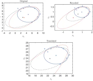
Fig. 1. Simulation example showing the invariance properties of the ALS1, ALS2, and orthogonal regression estimators. Dashed line—ALS1, solid line—ALS2, dashed dotted line—orthogonal regression,◦—data points,×—centers. Remark 32. Let T (x) = kSx+h with an orthogonal matrix S, and k = 0. Then for any sampleX,
D(T (X))=k2D(X).
In the next remark the similarity-invariance of the TALS estimator is concerned.
Remark 33. Consider the transformationTfrom Remark32. Denote the set of all the estimated link functions which are solutions to (43) by Sol2(X). Let1∈Sol2(X). Then1◦T−1is a solution to the problem (51), which is equivalent to
⎧ ⎨ ⎩
m l=1
2∗p
−k22(T (xl))→min,
k1()=1.
Then1k◦T−1∈Solk22(T (X)), and1(x)=0⇔1
k1(T−
1(T (x)))=0.
Hence, to introduce the similarity invariance, one has to take the rescaling of measurement error variance into account, and modify Definition25.
Transformations ALS1 TALS ALS2 Isometries preserving the origin Invariant Invariant Invariant
Translations Not invariant Invariant Invariant
Homotheties with the Not invariant Invariant if Invariant
center in the origin 2is rescaled
three estimators for the original data (example “special data” from[3]), for the data scaled by factor 0.2 and for the data translated by(20,20). We see that the ALS2 and orthogonal regression estimators are translation invariant and scale invariant, while the ALS1 estimator is not.
In the next table (see above) it is summarized whether an estimation problem is invariant for any sampleXagainst all transformations within a group.
6. Conclusion
We considered the implicit quadratic measurement error model in a Euclidean space, with normal errors. For the case of known variance, the similarity invariant version of the ALS estimator was presented and its strong consistency was shown. For the case of unknown variance, the consistency of the ALS2 estimators for the surface and the variance were proved under rather mild conditions. The ALS2 estimators are shown to be similarity invariant. We intend to generalize the results for unspecified error distributions.
Acknowledgements
The authors are grateful to two anonymous referees for valuable comments. Research sup-ported by Research Council KUL: GOA-Mefisto 666, IDO /99/003 and /02/009 (Predictive com-puter models for medical classification problems using patient data and expert knowledge), sev-eral PhD/postdoc & fellow grants; Flemish Government: FWO: PhD/postdoc grants, projects, G.0078.01 (structured matrices), G.0407.02 (support vector machines), G.0269.02 (magnetic res-onance spectroscopic imaging), G.0270.02 (nonlinear Lp approximation), research communities (ICCoS, ANMMM); IWT: PhD grants; Belgian Federal Science Policy Office IUAP P5/22 (‘Dy-namical Systems and Control: Computation, Identification and Modelling’); EU: PDT-COIL, BIOPATTERN, ETUMOUR. Part of the research was carried out when Sergiy Shklyar was vis-iting K.U. Leuven in 2003.
Appendix A. Proofs using the matrix representation ofqals
Proposition 34. The quadratic formqalsdefined by(9)is a solution to(8).
Before the proof of this proposition we consider the following identity.
Lemma 35. Forx ∼N (x,¯ 2I ),A∈S,b∈Rn var(xAx+bx)=24A2F +22Ax¯+b2. Proof. There exists a unique decomposition