AN IMAGE BASED FEATURE SPACE AND MAPPING FOR
LINKING REGIONS AND WORDS
Jiayu Tang, Paul H. Lewis
Intelligence, Agents, Multimedia Group, School of Electronics and Computer Science, University of Southampton, Southampton, SO17 1BJ, United Kingdom
[email protected], [email protected]
Keywords: Object Recognition, Image Auto-Annotation
Abstract: We propose an image based feature space and define a mapping of both image regions and textual labels into that space. We believe the embedding of both image regions and labels into the same space in this way is novel, and makes object recognition more straightforward. Each dimension of the space corresponds to an image from the database. The coordinates of an image segment(region) are calculated based on its distance to the closest segment within each of the images, while the coordinates of a label are generated based on their association with the images. As a result, similar image segments associated with the same objects are clustered together in this feature space, and should also be close to the labels representing the object. The link between image regions and words can be discovered from their separation in the feature space. The algorithm is applied to an image collection and preliminary results are encouraging.
1
INTRODUCTION
Image auto-annotation, which automatically labels images with keywords, has been gaining more and more attentions in recent years. It turns the tradi-tional way of image retrieval using low-level image features (colour, shape, etc.) as the query, into an ap-proach that is more favorable to people, namely us-ing words. However, many image auto-annotation techniques only generate labels at the whole image level, rather than at the object or region level. In other words, in this form auto-annotation does not indicate which part of the image gives rise to which word, so it is not explicitly object recognition. Discovering the relationships between image regions and partic-ular textual labels is the problem we wish to tackle in this paper.
1.1
Related Work
(Duygulu et al., 2002) view the process of image auto-annotation as machine translation. They first used a segmentation algorithm to segment images into object-shaped regions, followed by the construc-tion of a visual vocabulary, which is represented by
‘blobs’. Then, a machine translation model is utilized to translate between ‘blobs’ comprising an image and words annotating that image. Thus, it is capable of annotating objects in images.
(Yang et al., 2005) use Multiple-Instance Learn-ing (MIL) (Maron and Lozano-P´erez, 1998) to learn the correspondence between image regions and key-words. “Multiple-instance learning is a variation on supervised learning, where the task is to learn a con-cept given positive and negative bags of instances.” (Maron and Lozano-P´erez, 1998). Labels are attached to bags (globally) instead of instances (locally). In their work, images are considered as bags and objects are instances.
1.2
Overview of Our Approach
We propose an image based feature space and a map-ping of image regions and words into the space for object recognition. Firstly, each image is segmented automatically into several regions. For each region, a feature descriptor is calculated. We then build a fea-ture space, each dimension of which corresponds to an image from the database. Finally, we define the mapping of image regions and labels into the space. The correspondence between regions and words is learned based on their relative positions in the feature space.
The details of our algorithm are described in Sec-tion 2. SecSec-tion 3 shows experimental results and some discussions. Finally we draw some conclusions and give some pointers to future work.
2
IMAGE SPACE BASED
EMBEDDING OF REGIONS
AND WORDS
In this section, we first describe how image segments can be represented by visual terms which are based on salient regions. Secondly, we propose how to em-bed image regions and words into an image based fea-ture space, in order to find the relationships between words and image regions. Then, a simple example is presented as an illustration of the algorithm.
2.1
Representing image regions by
salient regions
There are very many different automatic image seg-mentation algorithms. In this work the Normalized Cuts framework (Shi and Malik, 2000) is used be-cause it handles segmentation in a global way which has more chance than some approaches to segment out whole objects.
Once images are segmented, a descriptor is calcu-lated for each image segment. The approach of (Tang et al., 2006) is followed to represent images by salient regions. Specifically, we first select salient regions by using the method proposed by Lowe (Lowe, 2004), in which scale-space peaks are detected in a multi-scale difference-of-Gaussian pyramid. Lowe’s SIFT (Scale Invariant Feature Transform) descriptor is used as the feature descriptor for the salient regions. The SIFT descriptor is a three dimensional histogram of gradi-ent location and origradi-entation. The descriptor is con-structed in such a way as to make it relatively invariant to small translations of the sampling regions, as might
happen in the presence of imaging noise. Quantisa-tion is applied to the feature vectors to map them from continuous space into discrete space. Specifically, the
k-means clustering algorithm is adopted to cluster the
whole set of SIFT descriptors. Each cluster then rep-resents a visual word from the visual vocabulary. As a result, each image segment can be represented by a k-dimensional frequency vector or histogram, for the visual words contained within the segment.
2.2
Image-Based Feature Mapping
We denote images as Ii(i=1,2, ...N,N being the total
number of images), and the jth segment in image Ii
as Ii j. For the sake of convenience, we line up all
the segments in the whole set of images together and re-index them as It ( t=1,2, ...,n,n being the total
number of segments).
We define an image-based feature mapping m, which maps each image segment into a feature space
F. The feature space F is an N dimensional space
where each dimension corresponds to an image from the data-set. The coordinates of a segment in F are defined by the mapping m:
m(It) = [d(It,I1),d(I t
,I2), ...,d(I t
,IN)] (1)
where d(It
,Ii) represents the coordinate of segment
It on the ith dimension for which we use the
dis-tance of It to image Ii. The distance of a segment
to an image is defined as the distance to the clos-est segment within the image. Because the number of visual words in a single segment can vary from a few to thousands, the distance between two vec-tors/histograms V1 and V2, which represent two
seg-ments, is measured by normalised scalar product (co-sine of angle), cos(V1,V2) =
V1•V2
|V1||V2|. Therefore, in this
work we define
d(It,Ii) =maxj=1,...,nicos(I
t
,Ii j). (2)
Intuitively, segments relating to the same objects or concepts should be close to each other in the feature space.
We can also map labels used to annotate the im-ages into the space. Suppose the vocabulary of the data-set is Wj( j=1,2, ...,M, M being the vocabulary
size). The coordinate of a label on a particular di-mension is decided by the image this didi-mension rep-resents. If the image is annotated by that label, the coordinate is 1, otherwise it is 0. Therefore, the map-ping of words is defined as:
m(Wj) = [d(Wj,I1),d(Wj,I2), ...,d(Wj,IN)] (3)
where
d(Wj,Ii) =
1 i f Iiis annotated by Wj
Ideally, a label should be close to the image seg-ments associated with the objects the label represents. The normalised scalar product is used to measure the distance between a segment and label, calculated as
cos(m(It)
,m(Wj)).
This mapping is similar to the work of (Bi et al., 2005), in which a region-based feature mapping is used. However, they defined a feature space in which each dimension is an image segment, and then map each image into the space. In other words, the two mappings are essentially the inverse of each other. However, one of the advantages of our mapping is that it is also able to map image labels to the feature space. For (Bi et al., 2005)’s mapping, there is no way to identify the coordinate of a label on each dimension of the feature space because labels are only attached on an image basis, rather than a region basis. In ad-dition, instead of using global features (colour, shape, texture), we use a histogram of visual words, which are quantised from salient regions within each image segment.
2.3
A Simple Example
In this section a simple example is presented to illus-trate the major steps of the method. Consider two an-notated images; I1is labelled as “RED, GREEN” and
half of the image is red and the other half is green;
I2is labelled as “GREEN, BLUE” and half is green
and the other half is blue. Assume the segmenta-tion algorithm manages to separate the two colours in each image and segments them into halves, we will have four segments in all, denoted as I1
,I
2
,I
3and I4.
Using the RGB values as the feature descriptors, the segments can be represented as I1= (255,0,0),I
2=
(0,255,0),I
3= (0
,255,0),I
4= (0
,0,255). Then we
need to map the segments into the feature space, which is a two dimensional space in this case as there are two images. By applying Equation 1, the coordi-nates of the segments are as follows:
I1: [1,0];
I2: [1,1];
I3: [1,1];
I4: [0,1];
(5)
In addition, the labels can also be mapped into the feature space to give:
RED : [1,0];
GREEN : [1,1];
BLU E : [0,1];
(6)
It can now be seen that in the feature space, the closest labels for the segments are:
I1: RED;
I2: GREEN;
I3: GREEN;
I4: BLU E;
(7)
3
RESULTS AND DISCUSSION
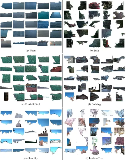
The method has been applied to the Washington im-age set1 which contains 697 semantically annotated images. After the original keyword labels were pro-cessed by correcting mistakes and merging plurals into singular forms (Hare and Lewis, 2005), the vo-cabulary consisted of 170 keywords. The whole set of SIFT descriptors are quantized into 3000 visual words. The number of segments is set to 5 per image when using Normalized Cuts (Shi and Malik, 2000). This results in 3241 segments after removing those having no salient regions within them. For each key-word, we find in the feature space the 25 closest seg-ments. The number of correct segments for each word is counted manually and those for the 25 key-words (Figure 1) with the highest occurrences in the data-set are reported in Table 1. Because of the fact that the original labels are only attached to the whole image, the decision of whether a segment is correct or not is made by human judgement. We consider a seg-ment being correct if the corresponding object occu-pies more than 50 percent of the area of the segment, otherwise not. Figure 3 shows some good examples, and Figure 4 shows some bad ones.
0 50 100 150 200 250 300 350 400 450 500 Tree Build ing Peop le BushGra
ss Clear
SkyWater Sky Clo udy Sky Flow er Side wal k
Rock Gro
und
Ove rcas
t Sky
Parti ally
Clo udy
Sky Hill Mou ntai n Stad ium Foot ball Fiel d
CarTrackPoleStand
[image:3.595.311.531.496.627.2]Leaf less Tre e Boat Occurrence Words
Figure 1: Top 25 Words that appear most frequently in the Washington set
As shown in Table 1, the results for some key-words are reasonably good, however, for the others
1Available at: http://www.cs.washington.edu/research/
they are less so. There are several possible explana-tions.
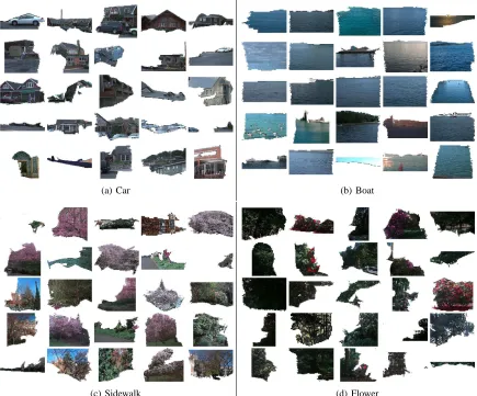
1. First of all, some objects are too small in the im-age to be segmented out reliably by a 5 region N-cut. For example, “Sidewalk”, “Car” and “Boat” usually occupy small areas of the image in the Washington set and rarely achieve good segmen-tations. Therefore, the algorithm returns the ob-jects that have a high co-occurrence with these words. For “Sidewalk”, image segments with “Trees” are found; For “Car” and “Boat”, seg-ments with “Building” and “Water” are found re-spectively, as shown in Figure 4.
2. Secondly, some words occur together almost ev-ery time they occur and rarely occur separately. This is analogous to an extreme example where a child who has never learnt what a knife and fork look like, is given many images in which both knife and fork appear together, even if he/she is told that all the images contains a knife and fork, there is no way for the child to learn which is which. In the Washington set, “Football Field”, “Track” and “Stand” co-occur almost totally. As shown in Figure 2, for each cell, the number on the dashed line indicates the number of times two words appear together (in the same image), and the other two numbers indicate their occurrence alone without the other. For example, “Track” and “Football Field” occur 36 times together, but only 1 and 7 times respectively on their own. Be-cause of high co-occurrence, the algorithm failed to distinguish them from each other. Almost the same results are returned for them, mostly “Foot-ball Field” as shown in Figure 3(c), which is prob-ably because the feature descriptors for “Football Field” are more stable.
3. Lastly, insufficient feature descriptors. Since the SIFT descriptor is using only grey level infor-mation, objects that are mainly distinguished by colour will be hard to identify. For example, in this work, the segments returned for “Flower” contain a lot of “Tree” labels (Figure 4(d)), prob-ably because in the data-set, the SIFT feature de-scriptors for both “Flower” and “Tree” are similar and also often co-occur as well.
4
CONCLUSIONS AND FUTURE
WORK
A novel image based feature space has been proposed together with a procedure for mapping in both im-age segments and textual labels. Some segments
as-Keywords Our Method Random
Tree 21 3
Building 22 0
People 21 1
Bush 25 3
Grass 6 1
Clear Sky 19 0
Water 25 2
Sky 19 3
Cloudy Sky 21 3
Flower 8 2
Sidewalk 2 0
Rock 6 2
Ground 6 3
Overcast Sky 0 3
Partially Cloudy Sky 20 4
Hill 0 2
Mountain 5 1
Stadium 22 0
Football Field 20 1
Car 7 1
Track 2 0
Pole 1 0
Stand 0 1
Leafless Tree 24 1
[image:4.595.320.511.85.360.2]Boat 0 0
Table 1: The number of correct segments out of the top 25 for our method and random choice.
Track Stand Football Field Track 5 30 7 7 36 1 Stand 7 30 5 9 34 1 Football Field 1 36 7 1 34 9
Figure 2: The number of times words “Track”, “Stand” and “Football Field” occur together and separately.
sociated with the same objects should be clustered together, and also close to the label that represents the object in question. As a result, the relation-ships between image regions and words can be dis-covered by comparing their distances in the feature space. Annotating new image segments and images is also straightforward by mapping them into the al-ready built space and finding the closest labels.
One current disadvantage of the approach is that the feature space has as many dimensions as anno-tated images in the set used to build the space. Ways in which the dimensionality of the space can be re-duced without losing the association between seg-ments, labels and images is being explored.
[image:4.595.347.483.399.492.2](a) Water (b) Bush
(c) Football Field (d) Building
[image:5.595.81.518.121.673.2](e) Clear Sky (f) Leafless Tree
(a) Car (b) Boat
[image:6.595.82.517.215.576.2](c) Sidewalk (d) Flower
and the use of richer feature descriptors than the SIFT. The approach will be tested on other image data-sets for comparison. Since the segmentation is particu-larly important in this approach, different approaches to segmentation will be evaluated, including in par-ticular, the multiple segmentation idea proposed by (Russell et al., 2006).
REFERENCES
Bi, J., Chen, Y., and Wang, J. Z. (2005). A sparse support vector machine approach to region-based image cat-egorization. In CVPR ’05: Proceedings of the 2005 IEEE Computer Society Conference on Computer Vi-sion and Pattern Recognition (CVPR’05) - Volume 1, pages 1121–1128, Washington, DC, USA. IEEE Computer Society.
Duygulu, P., Barnard, K., de Freitas, J., and Forsyth., D. (2002). Object recognition as machine translation: Learning a lexicon for a fixed image vocabulary. In The Seventh European Conference on Computer Vi-sion, pages IV:97–112, Copenhagen, Denmark.
Hare, J. S. and Lewis, P. H. (2005). Saliency-based mod-els of image content and their application to auto-annotation by semantic propagation. In Proceedings of Multimedia and the Semantic Web / European Se-mantic Web Conference 2005.
Lowe, D. G. (2004). Distinctive image features from scale-invariant keypoints. Int. J. Comput. Vision, 60(2):91– 110.
Maron, O. and Lozano-P´erez, T. (1998). A framework for multiple-instance learning. In Jordan, M. I., Kearns, M. J., and Solla, S. A., editors, Advances in Neural Information Processing Systems, volume 10. The MIT Press.
Russell, B. C., Efros, A. A., Sivic, J., Freeman, W. T., and Zisserman, A. (2006). Using multiple segmentations to discover objects and their extent in image collec-tions. In Proceedings of CVPR.
Shi, J. and Malik, J. (2000). Normalized cuts and image segmentation. IEEE Transactions on Pattern Analysis and Machine Intelligence (PAMI).
Tang, J., Hare, J. S., and Lewis, P. H. (2006). Image auto-annotation using a statistical model with salient re-gions. In IEEE International Conference on Multi-media & Expo (ICME).