Risk mapping in the Condamine River catchment basin

University of Southern Queensland

Faculty of Engineering and Surveying

Risk Mapping in the

Condamine River Catchment

Basin

A dissertation submitted by

Cameron Scott MacGregor

In fulfilment of the requirements of

Courses ENG4111 and ENG4112

Research Project

towards the degree of

Bachelor of Technology

(Geographic Information Systems)

Abstract

Erosion and Salinity are two of the most significant environmental problems impacting on agricultural lands in Australia. Currently 48000 hectares of Queensland are seriously affected by salinity, and an estimated 3100000 hectares of Queensland are also likely to be affected by the year 2050 (Gordon, I. 2002). When this is combined with approximately 20 to 60 tonnes of top soil per hectare being lost from cropping areas on an annual basis (Carey, B, Harris, P. 2001), it has become apparent that action needs to be taken. Through instigating efficient land management practices we must aim to prevent the formation of saline soils and water ways and at the same time limit the loss of top-soil through erosion.

A key tool in the management of salinity and erosion is the process of ‘risk mapping’. This tool has already been successfully used for salinity and erosion risk mapping as well as in other areas such as Fire Risk Mapping (Rural Fire Service, Queensland) and Forest Health Risk Mapping (Department of Agriculture, C’wealth).

Risk mapping uses input datasets which reflect environmental (both natural and human) attributes such as vegetation, soils, terrain, waterways, geology and rainfall. These data sets can be manipulated to show environmental indicators for various issues.

University of Southern Queensland

Faculty of Engineering and Surveying

ENG 4111 and ENG 4112 Research Project

Limitations of Use

The Council of the University of Southern Queensland, its Faculty of Engineering and Surveying, and the staff of the University of Southern Queensland, do not accept responsibility for the material associated with or contained in this dissertation.

Persons using all or any part of this dissertation do so at their own risk, and not at the risk of the Council of the University of Southern Queensland, its Faculty of Engineering and Surveying or the staff of the University of Southern Queensland. The sole purpose of the unit entitled “Project” is to contribute to the overall education process designed to assist the graduate enter the workforce at a level appropriate to the award.

The project dissertation is the report at of an educational exercise and the document, associated hardware, drawings, and other appendices or parts of the project should not be used for any other purpose. If they are so used, it is entirely at the risk of the user.

Prof G Baker Dean

Certification

I certify that the ideas, designs and experimental work, results, analyses and conclusions set out in this dissertation are entirely my own effort, except where otherwise indicated and acknowledged.

I further certify that the work is original and has not been previously submitted for assessment in any other course or institution, except where specifically stated.

Cameron Scott MacGregor Q12216129

Signature

Acknowledgements

Firstly I must acknowledge the Queensland Murray Darling Committee Inc. (QMDC) for providing the data used during the analysis stages of this project. Also my sincerest thanks are extended to my co-workers at QMDC who have provided wisdom and professional guidance throughout the year in both my project work and professional development.

I would also like to take this opportunity to acknowledge the support, guidance and professional manner of my project supervisor, Dr Sunil Bhaskaran, of the University of Southern Queensland. Throughout this project his advice, words of wisdom and support have proven to be in-valuable.

List of Figures

Page

Figure 2.1 - Arithmetic Overlay Operation: Addition ………. 6

Figure 2.2 - Weighted Overlay Process……….. 7

Figure 2.3 - ‘Model Builder’ – Diagrammatic Modeling Process……..… 8

Figure 2.4 - Role of Vegetation in maintaining ground water levels…… 13

Figure 2.5 - Rising Water Tables…………..……… 14

Figure 2.6 - Processes of Irrigation Salinity………...……. 16

Figure 2.7 - Three Forms of Wind Erosion……….. 19

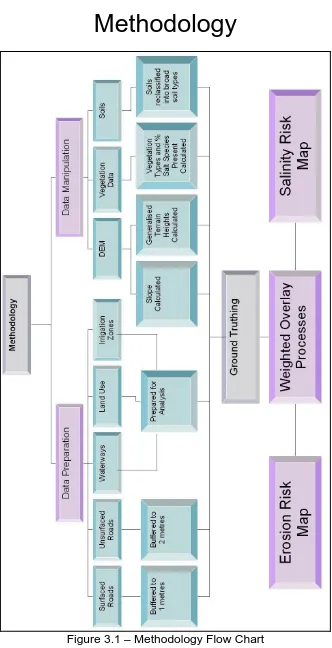
Figure 3.1 - Methodology Flow Chart……….. 22

Figure 3.2 - Study Area: Condamine River Catchment Area………..…. 24

Figure 3.3 - Common land uses within the CRCA………...… 25

Figure 3.4 - Land Use Composition………..…... 25

Figure 3.5 - Climatic Averages within the CRCA………... 26

Figure 3.6 - Ground truthing locations……….… 31

Figure 3.7 - Soil Record Photo (West of Pittsworth)……….. 32

Figure 3.9 - Slope Data-set (Percentage)………... 36

Figure 3.10 - Salinity Risk Model………... 40

Figure 3.11 - Vector to GRID Conversion………. 41

Figure 3.12 - Print Screen: Vector to GRID Conversion Setup…………. 41

Figure 3.13 - Salinity Risk Weightings……….. 42

Figure 3.14 - Erosion Risk Model: ‘Model Builder’……….. 44

Figure 3.15 - Erosion Risk Weightings……….. 46

Figure 4.1 - Salinity Risk Map………...… 50

Figure 4.2 - Erosion Risk Map………... 52

Figure C1 - Major Natural Features of the CRCA ………. 101

Figure C2 - Plants Suitable for Salt Soils……….... 102

List of Tables

Table 3.1 - List of base data-sets used in project………. 27

Table 4.1 - Salinity Risk Map Accuracy………..… 49

Figure 4.2 - Salinity Risk Statistics………... 50

Table 4.3 - Erosion Risk Map Accuracy………. 51

Table 4.4 - Erosion Risk Statistics……….. 52

Table of Contents

DISCLAIMER.………... iii

CERTIFICATION………... iv

ACKNOWLEDGEMENTS……… v

LIST OF FIGURES……….….. vi

CHAPTER 1 – INTRODUCTION

1.2 Rationale of Study……….. 2

1.3 Objectives………... 3

CHAPTER 2 – LITERATURE REVIEW

2.1 Introduction………. 5

2.2 Risk Mapping……….. 5

2.3 Weighted Overlays.……… 6

2.3.1 Model Builder……… 7

2.4 Salinity 2.4.1 Introduction……….. 10

2.4.2 Soil Salinity……….. 11

2.4.2.1 Salt Stores / Historic Salt………...…… 12

2.4.2.2 Ground Water Table Height………... 12

2.4.3 Dryland Salinity……… 15

2.4.4 Irrigated Salinity………...…… 16

2.5 Erosion 2.5.1 Introduction………..……… 17

2.5.2 Wind Erosion………..………. 18

2.5.3 Water Erosion………... 20

CHAPTER 3 – METHODOLOGY

3.1 Introduction……….. 23

3.2 Study Area…….……….. 23

3.3 Data Analysis……….. 26

3.4 Data Pre-processing 3.4.1 Data Projections...……… 28

3.4.2 Data Clipping...………. 28

3.4.3 Ground Truthing………... 29

3.4.4 Vegetation Data……… 33

3.4.5 Soils Data……….. 34

3.4.6 DEM Derived Data…….……….. 35

3.4.7 Roads and River Network Data………. 37

3.5 Data Processing 3.5.1 Introduction……… 38

3.5.2 Salinity Risk Map….………. 38

3.5.3 Erosion Risk Map……..………... 43

3.6 Summary………. 47

CHAPTER 4 – RESULTS

4.1 Introduction……….. 48

4.2 Results: Salinity Risk Map………..……….. 48

4.3 Results: Erosion Risk Map…….……….. 51

CHAPTER 5 – DISCUSSION

5.2 Data Pre-processing 5.2.1 Ground Truthing…...……… 53

5.2.2 Soils Generalisation………. 55

5.2.3 River and Road Buffering………... 56

5.2.4 Regional Ecosystems Data……… 58

5.2.5 Potential Data-Sets……….. 58

CHAPTER 6 – CONCLUSIONS &

RECOMMENDATIONS

6.1 Introduction……… …..61

6.2 Conclusions….……….. 61

6.3 Recommendations 6.3.1 Introduction……...……… 62

6.3.2 Recommendations for Usage.……… 62

6.3.3 Recommendations for further Action…….. ……... 63

6.3.4 Recommendations for further Study……... 64

6.4 Summary…..….……….. 64

REFERENCES

APPENDIX A

APPENDIX B

Chapter 1

Introduction

1.1 Introduction

With salinity and erosion becoming more evident in agricultural areas of Queensland it is essential that the remaining ‘quality land’ is preserved and not allowed to degrade further. At the same time, it is imperative that relevant stakeholders manage and rehabilitate land already severely affected or under threat of becoming degraded.

The main method of managing land to ensure that further degradation is avoided is to initiate stringent management plans which invest in strategic rehabilitation or land management. This management can be achieved efficiently through the use of risk maps (sometimes known as hazard maps).

1.2 Rationale of the Study

The rationale of this study as mentioned in Section 1.1 of Chapter 1 is to use the process which is referred to in this project as risk mapping to map the susceptibility of a selected area of land (through the use of environmental indicators) to environmentally degrading processes such as salinity and erosion.

1.3 Objectives

This project encompasses a number of broad objectives ranging from the conducting of research into the environmental issues of salinity and erosion through to investigating and using GIS software to create risk maps. A more in-depth and complete list of the objectives of this project are:

To conduct research into the environmental and economical effects of salinity and erosion

To document and evaluate available software which are used for assessing risk

To ground truth datasets and determine the accuracy of input data-sets;

1.4 Scope and Limitations of the study

This study is conducted using available GIS data to model risk in the Condamine River Catchment Area. Therefore the accuracy of the results presented in this study is only true as the quality and accuracy of the data used. However despite the limitations in regards to input data-sets, the scale at which they are useful at and accuracy, they have enabled a broad understanding of the risks in the Condamine River Catchment Area. Data-sets (relating to environmental indicators) have not been included in this project since they were not available at the commencement of this project.

Chapter 2

Literature Review

2.1 Introduction

The purpose of this literature review is to provide back ground information for the processes modelled during this project. Therefore information presented in this chapter is directly linked with later chapters of this dissertation. The following information has formed the knowledge base for decision making in regards to reclassifying datasets to accurately show the potential risk of land to salinity and erosion.

2.2 Risk Mapping

Risk mapping is a mapping process which is described by the name which the process is given. Risk mapping is the process of mapping potential risk from any given number of scenarios of situations in a visual manner. Risk mapping generally provides output in the form of data which can be reclassified into a percentage or other form of ranking which can then be used to show the level of risk associated with a process.

2.3 Weighted Overlays

The weighted overlay process has many applications. Due to the topic of this project, this chapter will only focus on relevant sections of this process.

The overlay process can be conducted with either vector or raster data, however for the purposes of this dissertation, vector overlays will not be considered as they are too time consuming and there is the risk of creating many sliver polygons within an area such as the study area for this project. Therefore this section will focus on introducing the processes associated with the overlay of raster data within a GIS environment.

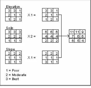
The overlay of raster data involves the “overlaying of GRID cells of one raster layer to another layer (See Figure 2.1) (Apan, A, 2003, p 5.13) using a common evaluation scale”. (Model Builder Help: Overlay Process, 2000) This common evaluation scale is comprised of numbers which are assigned by the user.

Figure 2.1 - Arithmetic Overlay Operation: Addition (DeMers, 1997, p.331 in Apan, A, 2003, p 5.14)

This ability for a user to use particular data-sets to influence the output data can be seen in Figure 2.2 below. In this example the soils input layer is given a higher rating than the elevation and slope data, hence giving it a greater influence on the output data.

Figure 2.2 – Weighted Overlay Process

ch Institute) (It is also an addition to the Spatial Analyst Extension in ArcGIS 9). It provides

the e

presented in a graphical manner through the use of flow charts/tree diagrams (See Figure 2.3).

(Davis, 1996, p.234 in Apan, A, 2003, p 5.20)

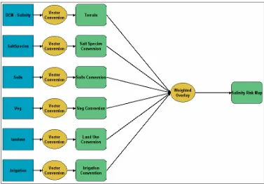
2.3.1 Model Builder

‘Model Builder’ is a component of the ‘Spatial Analyst 2.0 Extension’ for the GIS platform, ‘ArcView 3.2’ which is a product of ‘ESRI’ (Environmental System Resear

Figure 2.3: ‘Model Builder’ – Diagrammatic Modelling Process

his diagrammatic representation of modelling procedures within odel Builder’ provide a number of advantages. These dvantages range from it being reusable and shareable with

el Builder Help: hat is Model Builder?, 2000) as well as allowing users to run components of models individually to reduce processing time. T

‘M a

others, providing easy modification of models to explore "what if" scenarios, to obtaining different solutions (Mod

‘Model Builder’ incorporates an extensive range of data manipulation and conversion functions including:

Vector to GRID Conversion DEM to GRID Conversion Point Interpolation Slope Calculation

ulation

GRID Reclassification

During the course of this project two data manipulation procedures were undertaken within the ‘Model Builder’ environment to create the salinity and erosion risk maps. These procedures were ‘Vector Conversions’ and ‘Weighted Overlays’. However a number of other processes could have been incorporated into the

luding:

Buffering

l preference. Aspect Calc

Hillshade Calculation Contour Calculation

Buffering

Arithmetic Overlays Weighted Overlays

to GRID

modelling processing inc

Slope Calculation; and DEM to GRID Conversion.

2.4 S

alinity is a form of extreme environmental, social and economical egradation. However it must be noted that salinity or salinisation a natural environmental process, this process has led to significant salt storages within the non saturated zone of ueensland soils”. (Working Party on Dryland Salting in Australia,

alinity costs the national economy $200 million annually through

ant when the current estimates for 2050 f areas seriously affected is 3.1 million hectares, an increase of

alinity

2.4.1 Introduction

Salinity is a term used to describe the salinisation (“the accumulation of salts in soil” (Miller, G, T, 2004, p G13)) of soils and waterways. For the purposes of this research project the term salinity will refer to only the processes of soil salinisation, as the study area for this project is inland as well as their being insufficient waterways information to model the potential risk of rivers to salinity.

S d is ‘’ Q

1982, p 12)

S

lost revenue (Warnick, 2003). Currently there is an estimated 48000 hectares of land in Queensland which is seriously affected by salinity. (Gordon, I, 2002) Whilst this area may seem insignificant in the scope of a state the size of Queensland, it doesn’t seem so insignific

o

2.4.2 Soil Salinity

gnised that there are two forms of soil salinity; they are Dryland Salinity and Irrigated Salinity. These forms of soil salinity are y

between the two forms of salinity being human induced environmenta

The level of severity at which each of these two forms of soil salinity form at is dependent on a number of factors including the salt:

stored in the groundwater tables stored in the soil profile; and in the water used for irrigation

Other major factors which contribute to the formation and severity of salinity include:

the position or depth of the ground water table in

it is)

rainfall Levels It is generally reco

ver similar with the only distinguishing difference

l activities.

the soil profile

the state of the environment (i.e. whether vegetation is present and what sort of vegetation

land use practices; and

2.4.2.1 Salt Stores / Historic Salt

In Australia there are significant stores of existing salt in the unsaturated and saturated (water table) sections of the soil profile. This has been the result of ongoing environmental processes

cluding:

the weathering of parent material (rocks) over

ground water tables.

t on egetation growth and health. It is through human induced actions uch as irrigation and tree clearing that these salt stores are able

rise higher in the soil profile.

ater present in the water table as ell as the depth of shallowest layer of impermeable bedrock in

time and the subsequent release of salt stored in the parent material

the depositing of salt from sea mist; and the intrusion of salt water into the fresh

In most cases the existing salt stores in Australian soil profiles are deep enough to ensure that they have little to no impac v

s to

2.4.2.2 Ground Water Table Height

The height of the ground water table in the soil profile is determined by the volume of w

w

(prevent water from filtering further down in the soil profile).

The processes by which the ground water tables rise as a result of irrigation salinity are fairly simple as there is a localised increase of water entering the soil profile as a result of irrigation. However implications of tree clearing and the associated rise in ground water tables is more complex.

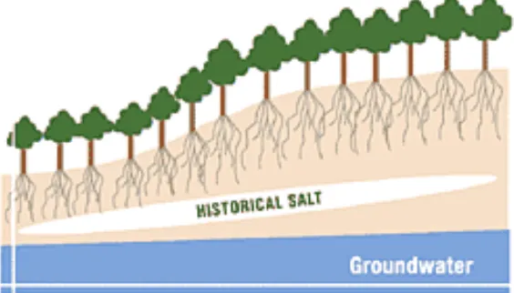
Vegetation (particularly deep rooted native vegetation) plays a major role in the extraction of water from the soil profile through the process of transpiration. This extraction of water from the soil p

any recharge is kept at equilibrium so that water tables stay at approximately the same level (See Figure 2.4).

rofile generally ensures that the extraction from water tables and

However once the trees are cleared from an area the rate of recharge is generally higher than the rate of extraction through either transpiration or evaporation. This will cause the water tables

rise over time (See Figure 2.5). to

Figure 2.5 – Rising Water Tables (Fitzroy Basin Association, 2004)

The effects of clearing vegetation become more apparent in the hort and long term if the clearing is conducted in areas of a zones. These zones are where the majority of the water, which makes its way to the groundwater

ers the landscape. (A technical definition describes

ile and bring with it the salts from lower in the s

catchment known as recharge

tables ent

recharge zones as “the area in a catchment where the net movement of water is downwards to the groundwater.” (Ghassemi, F, et al, 1995, p 516))

This means that the water tables in that catchment are more likely to rise at a quicker rate as there is less deep rooted vegetation in the soil profile to extract water before it reaches the ground water table. This means that over time the ground water table will rise within the soil prof

Over time if left un-checked, the increased infiltration of water into e ground water tables can cause the tables to rise to the point at they infringe on the root growth zone of plants (See Figure .5) or in some cases to the surface of the soil (saline seeps). This reates conditions in which a majority of vegetation is unable to urvive.

.4.3 Dryland Salinity

ryland Salinity is a process heavily influenced by the clearing of egetation as mention earlier in this chapter. In the case of dryland alinity it is caused by the clearing of trees for cropping and

allows an increased flow of water to the ground water tables over time causing the ground water th

th 2 c s

2

D v s

grazing. The clearing of trees in

2.4.4 Irrigated Salinity

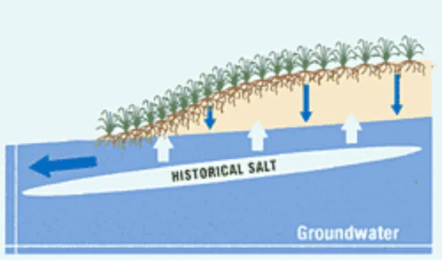
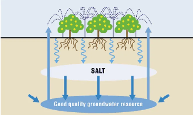
Irrigated salinity unlike dryland salinity can occur even if tree clearing has not occurred. This is because large quantities of water are being applied directly to the landscape on a regular basis. This water filters directly to the ground water table (See Figure 2.6) and will cause it to rise higher in the soil profile.

Figure 2.6 – Processes of Irrigation Salinity

(Australian Government – National Action Plan for Salinity and

ble is considerably lower in the soil profile. Water Quality, 2004)

2.5 E

rosion is “the detachment, entrainment, transportation and eposition of soil and other earth materials” (Toy, T.J, Foster, G.R,

enard, K.G, 2002, p 1) by the actions of wind and water in onjunction with gravity.

able of destroying the productivity of the nd in just a few years or even months” (Toy, T.J, et al, 2002, p1).

ccurring process its destructive ower can and is increased as a result of human activities such as

rosion

2.5.1 Introduction

E d R c

The process of erosion is both naturally occurring and essential to shaping of the earth and is “largely responsible for the shape of the earths land surface today” (Toy, T.J, et al, 2002, p1). Erosion is considered to be one of the most essential yet destructive process on earth as on one hand it is responsible for the breakdown of parent material (rocks) which in turn forms new soils and yet on the other hand it is “cap

la

Whilst erosion is a naturally o p

Erosion is a complex process and like salinity, its formation rates nd severity is dependent on a number of factors including egetation cover, land use practices, soil structure and terrain lope and length. The individual process of both wind and water erosion and how the above mentioned contributing factors

influence the following

sections of this chap

reater than the resistance of the soil to these forces oy, T.J, et al, 2002, p43). The resistance levels of soils depend

spension transport modes” (Toy, T.J, et al, 2002, p44) (See igure 2.7)

a v s

severity of erosion will be discussed in the ter.

2.5.2 Wind Erosion

Wind erosion is caused when the forces applied to the soil by the wind are g

(T

on the level of moisture present in the soil profile, this is because moisture binds soil particles together increasing their resistance to wind erosion. Therefore wind erosion rates are generally low when there is a high level of soil moisture and high when soil moisture content is low.

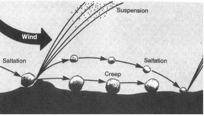
There are “three forms of wind erosion; these are creep, saltation and su

Figure 2.7 – Three Forms of Wind Erosion l, 2002, p44)

The ‘transpor i ’ is a process where larger sized earth/soil particles are pushed along the ground without

ss whereby lighter particles of arth/soil ‘skip’ across the surface of the land and become

large areas of exposed soils due to a lack of vegetative (Toy, T.J, et a

tat on mode’ named ‘creep

becoming airborne (See Figure 2.7) (this is due to the weight of the particles).

‘Saltation’ is a wind erosion proce e

airborne as a result of coming into contact with small irregularities in the landscape often dislodging further particles (See Figure 2.7). Finally the ‘transportation mode’ of ‘suspension’ is when the finer earth/soil particles become completely airborne and are transported across the landscape in giant dust storms (See Figure 2.7).

Wind erosion is most likely to occur in drier landscapes where there are

2.5.3 Water Erosion

Water erosion is the most predominant form of erosion in Australia nd is caused by the “stresses generated by rain drop impact, and

s of water erosion which occur the environment, these forms include:

Rill Erosion

ank Erosion

egetation serves two purposes in the prevention of water erosion. irstly the foliage of vegetation acts as a barrier between rain rops and the soil surface. This barrier does not altogether prevent

indrops from reaching the soil surface but rather reduces the velocity at which the rain drops hit the soil surface. Vegetation roots also serve ing as a stabilisation mechanism which aids in holding the soil profile together and reduces the sus to all forms of water erosion.

a

surface runoff” (Toy, T.J, et al, 2002, p25). Therefore water erosion can be described as the detachment, entrainment, transportation and deposition of soil and other earth materials through the process of the hydrological cycle.

There are a number of different form in

Tunnel Erosion Mass Movement Sheet Erosion Gully Erosion; and Stream B

However due to the modelling of erosion as a generalised form of degradation in this project the remainder of this section on water erosion will be dedicated to outlining the impacts of vegetation, soil and slope on water erosion rates.

V F d ra

the purp se of acto

The size of the soil particles in the soil profile also dictates the susceptibility of the soil profile to erosion with smaller soil particles being at greater risk of erosion than large particles. This is because larger soil particles have a greater mass and hence require water movement of a greater force to move them (i.e. sandy soils (finely grained) will be at greater risk of erosion than clay soils (coarsely grained) due to the relative difference in soil particle size)

Slope is another critical factor in determining the force of the water on the landscape. As water travels down a slope it picks up velocity and hence has a greater potential to cause erosion. The length of a slope also plays a role in the erosion rates of an area. For example a long moderate slope may have the same potential for erosion as a short steep slope.

2.6 Summary

When using environmental data-sets to map the potential risk of a particular area to forms of environmental degradation or any form of degradation or danger in general, it is essential to have a complete and thorough understanding of all literature regarding that form of degradation.

Therefore it was the aim of this chapter to provide sufficient information in regards to the degrading processes of salinity and erosion so that both the readers and the author of this dissertation have sufficient knowledge of the processes in order to understand

Chapter 3

Methodology

3.1 Introduction

This chapter is devoted to explaining, in detail, the data manipulation and processing steps that occurred through the course of this project, as well as documenting the role ‘Model Builder’ an extension of ‘ArcView 3.2’, played in this project.

3.2 Study Area

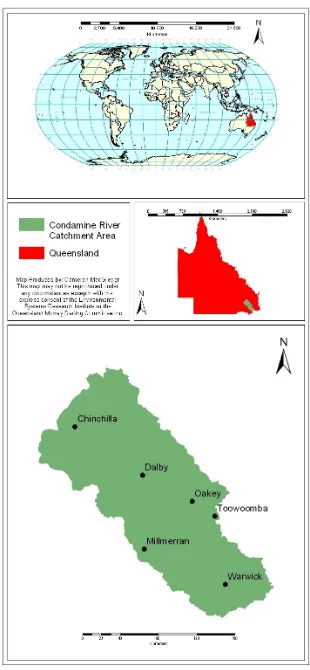
tchment area for the Condamine River which is dominant natural feature running down the centre of the study area (See Figure C1, Appendix C). Hence for the purposes of this dissertation the study area for this project will be referred to as the Condamine River Catchment Area or the CRCA.

The study area that was selected for this project is in the South Eastern corner of Queensland, Australia (See Figure 3.2). The area is made up of 15 smaller sub-catchment areas covering a total area of approximately 24434 km2. The study area can be best described as the ca

Due to the size of the study area there is a wealth of background information which could be included within this chapter, however to keep this chapter concise the information presented is only relevant to the topic of this project.

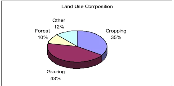
The CRCA is mainly an agricultural area comprising of vast tracts of grazing and cropping land. Typical scenes which may be encountered in the study area are shown in Figure 3.3 below.

Figure 3.3 - Common land uses within the CRCA

The percentage of land use within the CRCA varies; with cropping and ing approximately 78% (See Figure 3.4) of the

total lan te and

ational Forests consuming approximately 10% of the land. Other nd uses include such activities as urban, industrial, piggeries, nd poultry (12%).

grazing consum

d area or approximately 19058 km2. With Sta N

la a

Land Use Composition

Cropping 35% Other

Grazing 43% Forest

10% 12%

d Use Composition

Climatic conditions within the CRCA vary due to the large size of the area. However with respect to salinity and erosion the following table (Figure 3.5) represents core information regarding rainfall, evaporation and minimum and maximum temperature averages on an annual basis.

Category Averages

Rainfall 600 to 800 millimetres

Evaporation Between 1800 and 2400 millimetres Minimum Temperature 6 to 16 degrees

Maximum Temperature 21 to 27 degrees

Figure 3.5 - Climatic Averages within the CRCA (Bureau of Meteorology, 2004)

3.3 D

were two distinct stages which were conducted in order to produce the output salinity and erosion risk

data pre-processing; and

Data preprocessing was defined by converting data to the correct

the ‘Model Builder’ environment and setting weights

for pre-processing hilst a high performance computer was used during the weighted

ze of some of the GRID data-sets.

ata Analysis

During this project there

maps. These stages were:

data manipulation

coordinate systems as well as modifying it to realise its full potential. The data manipulation stage was categorized by adding the data into

to various data-sets.

For the analysis processes of this project two separate computers were used. A standard computer was used

w

The specifications for the computers used during the analysis stages of this project are:

1. Data Pre-processing

Pentium 4, 2 GHz Processor, 512 Mb RAM 2. Data Manipulation

Pentium 4, 2.4 GHz Processor, 1024 Mb RAM

The data use n

sources includ ntal Protection Agency, Department o

Merz, GeoScienc ommonwealth Scientific Industrial Research Organisation). However all data was made d i this project originated from a variety of different

ing the Environme

f Natural Resources and Mines, Sinclair Knight and e Australia and CSIRO (C

&

available by the Queensland Murray Darling Basin who has full access to the data. A list of data used in this project can be found in Table 3.1.

Data Name Point Line Polygon Raster Other

Vegetation (RE) Table

Surface Roads

Unsurfaced Roads

Soils

DEM

Land-use

Irrigation

River Systems

3.4 Data Pre-p

This section is d o outlining the processes of this project s well as the steps that were taken in order to prepare the data

mon projection chosen for this project as GDA 1994 (Geocentric Datum of Australia) MGA (Map Grid of ustralia) Zone 56. This was because all study areas for this roject fell into Zone 56 of the Map Grid of Australia.

order to re-project the data used in this project the following rojection software was used; ‘ArcView 3.2 – Projection Utility’.

.4.2 Data Clipping

preliminary stage of this project was to clip available data to the RCA extent. This served a number of purposes including a:

ipping for this project, the data torage space was roughly only a quarter of what it was previously.

rocessing

edicated t a

for use in weighted overlay stages of this project.

3.4.1 Data Projections

An essential step in overlay and other analysis procedures is to ensure that all data used as inputs is in the same projection. If data-sets are not in the same projection they will not project to the same place on the earth and hence will not be able to be used in analysis. Therefore the first stage of this project was to find out what projections the data was in and then to re-project it to a common projection. The com

w A p In p

3

reduction in data storage requirements; and reduction in time required to complete analysis

This stage wa n Model as it was missing certain files that ‘ArcView 3.2’ required. Therefore it was reclassified in ‘ArcGIS 8.3’ and converted to a ‘shapefile’; this shapefile was then clipped to the study area.

necessary component of any analysis procedure is to determine how accurate

project is being

ensure certain s f accuracy by setting strict standards for -existing data is being used, it is of termine the accuracy of data unless:

plete and reliable metadata exists

extensive ground truthing is undertaken to assess the accuracy of data-sets

Ground truthing generally involves going to planned locations within the study area for a project and recording all environmental or physical attributes from that location required for the assessment of data being used in the project.

s also necessary for the Digital Elevatio

3.4.3 Ground Truthing

A

the data being used is. If the data being used in the collected as part of the project it is possible to tandards or levels o

data collection. However if pre ten very difficult to de

Ground truthing generally can occur in two manners, both these can provide information to determine a reasonable measure of accuracy. The methods of ground truthing data are to:

ground truth the data by visiting locations to provide full coverage of all attributes in each data-set; or

ground truth the data by visiting locations which ensures that the study area is adequately covered.

The ideal method of ground truthing would be a combination of the above mentioned methods. This is because it is necessary to check both the attribute and positional accuracy to ensure that the data is consistent across the entire study area.

Ground truthing for this project occurred throughout the project tudy area; it involved visiting 27 locations through out the CRCA nd covering a distance of over 600 kilometres. (See Figure 3.6) s

a

For more detailed information regarding data collected during ground truthing see Appendix B.

At each location a number of attributes were recorded in accordance with data-sets being used in the analysis stages of this

roject. The attributes recorded included:

Distance to Roads and Rivers (if visible) Slope; and

p

Latitude, Longitude and Height (above MSL (Mean Sea Level)) of the location using a Trimble GPS Unit (‘GeoXT’)

Soil Type (See Figure 3.7) Vegetation Type

Land-Use

Photograph and image direction.

Figure 3.7 – Soil Record Photo (West of Pittsworth)

At these points it was opted to physically record the attributes using pen and paper rather than organizing data dictionaries in the GPS (Global Positioning System) Unit. This was because it was determined that whilst in the field, attributes could be recorded in a

horter period of time, hence allowing for more locations to be

copy data from the GPS unit across to a computer using the ‘Terra Sync’ software developed by ‘Trimble’.

s

Upon comple

converted to a ‘s corded attributes were entered into the ‘shapefile’s’ attribute table. This information was

tion Agency. This data consists of two core gional Ecosystems’ (RE01) listing and a s of unique identifiers which are us professionals and experts, and a Microsoft Exc et (Comma rated) containing the ‘bulk’ or in-depth infor

vegetation patches to dominant v Grass Land etc.).

For the vegetation data to be consi

information sources for a more s thought that the two tables (dbf with the ‘RE’ shapefile and the joined in the ArcGIS environment.

‘RE Description’ olumns (most important source of information) were shortened to ting the ground truthing, recorded GPS points were

hapefile’ and physically re

then compared to the existing data-sets; from this a level of certainty was determined.

3.4.4 Vegetation Data

The vegetation data used for this project originated from the Environmental Protec

elements; a ‘shapefile’ officially titled ‘Re basic information serie

eful mainly for

el Spreadshe Sepa

mation in regards to species present within egetation types (Open Woodland,

dered of any use for this project it was necessary to combine both

‘complete’ data-set. Initially it wa (data base file) file associated spreadsheet) could be simply

However due to the immense volume of data present within the ‘RE’ spreadsheet, the tables were joined but the

c

Therefore it was determined that the primary process of information amalgamation would be conducted manually in a Microsoft Excel Environment. In this environment the following information was extracted for all vegetation patches within the CRCA:

species name

dominant vegetation type (See Appendix C for list) total number of species; and number of salt tolerant species.

racted information was then extracted and added into the ttribute table of the ‘RE’ data.

.4.5 Soil Data

he soils data used in this project used a base layer which is his data was extracted from the Atlas of ustralia Soils which consists of 1:100,000 map sheets and is . The soils information in this data-set is ategorized by soil descriptions described in the Atlas of Australian Upon the extraction of species names from the detailed vegetation descriptions, these were then searched using a list of salt tolerant vegetation species (See Appendix C) compiled by the Department of Natural Resources and Mines (Wright, A, Egan, S, Westrup, J, Grodecki A, 2001). The number of salt tolerant species for each patch was then counted, and compared as a percentage with the total number of species present for all vegetation patches. This ext

a

3

T

known as Md_Soils. T A

maintained by the CSIRO c

These soils types where then reclassified into the broader soil types of Clay, Loam and Sand. This reclassification was based upon soil descriptions provided in the Australian Agricultural

ssessment 2001 which provided information on soil types and as utilized and soil types were classified into the categories (mentioned above) based upon

owever it must be noted that this reclassification may not be as accurate, as the information used for the reclassification was based upon i lines. However due to a lack of in-depth information being available regarding soil composition little choice was left but to reclassify in ed way based upon available literature.

f the data-sets were created for use during analysis and ill be discussed in this section however other data-sets were reated purely for map aesthetics such as the hillshade which can

the Spatial Analyst xtension for ArcGIS 8.3, these operations involved the:

a Slope Raster

the DEM into more defined changes in terrain height.

A

attributes. This information w re

what component (i.e. Sand, Clay, Loam) was dominant in the soil type.

H

nat onal categorization guide

for this project area, the above mention

3.4.6 DEM Derived Data

During the course of this project two data-sets were derived from the DEM (Digital Elevation Model) used for this project. The majority o

w c

be seen in Appendix C, Figure C1.

Two operations were conducted using E

creation of

Each of these files was created with an output resolution of 25 metres. This was because the accuracy of the input data-set was plus or minus 25 metres. The slope file was then reclassified to allow for easier use in ‘Model Builder’. The percentage slope values were then reclassified into broader categories which can be seen below in Figure 3.8. The results of this reclassification can be seen in Figure 3.9.

Figure 3.8 – Slope Reclassification Values

Figure 3.9 – Slope Data-set (Percentage) New Value Old Value

3.4.7 Roads and River Network Data

Roads and river systems data were used in this project. However they were only used in the creation of the erosion risk map. The use of these data-sets may however have implications for assessing the potential danger of infrastructure from high salt levels through processes such as ‘salt cancer’.

The road data consisted of two ‘shapefiles’, one showing surfaced roads and the other showing un-sealed roads. These data-sets were ‘buffered’ to 1 and 2 metres respectively. These buffered areas were considered to be areas most at risk of erosion. However no evidence was found clearly documenting relationships between the type of road (i.e. surfaced, unsealed) and rates of erosion at critical distances from road networks. Also the original data-sets were represented by ‘polyline’ features and no records were kept of road width and quality, (all of which may have an influence on run-off/erosion patterns).

3.5 Data Processing

3.5.1 Introduction

During this project all the data processing occurred within a component of the ‘ArcView 3.2’ Extension, ‘Spatial Analyst 2.0’ called ‘Model Builder’ (See Chapter 2.3.1).

Therefore this section will be devoted to explaining how ‘Model Builder’ was used and how weights were assigned to values within data-sets.

3.5.2 Salinity Risk Map

This component of the data processing saw the use of six data layers in a weighted overlay process in Model Builder. These data layers were:

Salt Tolerant Vegetation

Irrigation Areas

E t was lo a

another ‘shapefile’ containing an e CRC which was used to set the extent (“the area arth's surfac covered by the data used” (Environmental Research Inc. 2000)).

Soils Data

DEM

Vegetation Type Land-use; and

ach data-se aded into n ‘ArcView 3.2 Project’ as well as outline of th A

on the E e

I the model builder nvironmen of varia s were set under the ‘model defaults’ menu before any data layers were added to the model. These variables were:

extent cell size evaluation scale

The extent, as mentioned on th vious page w set to the boundary of the CRCA. The ce to 25 etres as it was the resolution of the DEM and the only documented level of accuracy for all data-sets. The evaluation scale for this project was set as ‘1 to 5’ (1(Low Risk) to 5 ) this w because it was thought to be the largest sca e used based upon the depth of data-set attributes. etting of the efaults, the data layers were then added into ling envi See Figure 3.10)

n e t a number ble

.

e pre as

ll size was set m

(High Risk) as le that could b

After s d

Figure 3.10 – Salinity Risk Model

hese layers then had the relevant attribute selected as the ategory to be used in the ‘Vector to GRID Conversion’ process

ee Figure 3.11). T

Figure 3.11 – Vector to GRID Conversion

this process each data set was given a new name which was en given to the output GRID data-sets (See Figure 3.12).

In th

Figure 3.12 – Print Screen: Vector to GRID Conversion Setup

e eries of ‘scales’ (1 to 5) and ‘%influences’ During the weighted overlay process these GRID files wer weighted using a s

Input Theme %Influence Attribute Name Scale Value High Risk 5

Moderate Risk 3 Low Risk 2 No Risk 1 Salt Toleran

Vegetation

20

No Data Restricte t

d

Clay 5 Loam 3 Sand 1 Soils 10

No Data Restricted Fern Thicket 3

Clear 5

Open Forest 2 Open Woodland 2 Rain Forest 1

Shrubland 3 Tall Open Forest 1

Vine Forest 3 Vine Thicket 3

Wetlands 4 Woodland 1 Vegetation Type 30

No Data Restricted

Cotton 5 Cropping 4 Dairy 3 Forestry 1 Grazing - Cattle 4

Grazing - Sheep 4

Industry 3 Irrigated Cropping 5

National Park 1 Grazing - Other 4

Piggery 3 Poultry 3 State Forest 1

Unclassified Restricted

Urban 2

Water Body Restricted Land-use 5

No Data Restricted Irrigation 5 Irrigation Areas 5

Restricte

No Data d

High Risk 5 Moderate Risk 4 Low Risk 3 Little to No Risk 1 DEM 30

No Data Restricted

These weights were then used to combine the input GRID data-sets in the weighted overlay process (See Figure 2.2) to create the

3.5.3 Erosion Risk Map

he process used to create the erosion risk map was very similar the process used to create the salinity risk map. This is largely ue to the similarities in the way each form of degradation forms. he major difference between these two weighted overlay rocesses is that some sets were removed and other data-ets replaced them to form the erosion risk model. In all, eight data

yers were used during this analysis stage (See Figure 3.14). hese values were:

Un-sealed roads Surfaced Roads Soils

Vegetation Type Land-Use

Irrigation Areas Rivers; and

Slope (derived from DEM) output/salinity risk map.

Upon completion of the weighted overlay process the output GRID was converted to ‘shapefile’ format. This ‘shapefile’ was then used in conjunction with the CRCA ‘shapefile’ to remove the ‘Restricted’ values which resulted from the rectangular shaped extent polygon created by ‘Model Builder’.

Due to large similarities between this erosion risk map and the linity risk iscu of th es t ed

this project will not be discussed; instead this section will focus on the weightings assigned to the data-sets in the erosion modelling. The modelling process for the eros isk map, like the salinity risk map used CRC undary s extent, ize of 25 metres and a rating scale of 1 to 5 for ‘layer’ attributes. The weightings an le v for the erosion risk map can be seen in Figure 3.15

sa map, d ssion e process hat occurr during

ion r

the A bo as it a cell s

Input Theme %Influence _{Attribute Name Scale Value} Steep Slope 5 Moderate Slope 3 Little to No Slope 1 DEM 25

No Data Restricted

Clay 1

Loam 3

Sand 5

Soils 10

No Data Restricted Fern Thicket 4 Clear 5 Open Forest 3 Open Woodland 3 Rain Forest 3 Shrubland 3 Tall Open Forest 2 Vine Forest 3 Vine Thicket 3 Wetlands 4 Woodland 2 Vegetation Type 30

No Data Restricted Cotton 4 Cropping 4 Dairy 3 Forestry 2 Grazing - Cattle 3 Grazing - Sheep 3 Industry 2 Irrigated Cropping 4 National Park 2 Grazing - Other 4 Piggery 4 Poultry 4 State Forest 2 Unclassified Restricted Urban 2 Water Body 1 Land-use 5

No Data Restricted Irrigation 4 Irrigation Areas 5

No Data Restricted Un-sealed Roads 4 Un-sealed Roads 10

No Data Restricted Surfaced Roads 2 Surfaced Roads 5

No Data Restricted Rivers 4 Rivers 10

No Data Restricted

3.6 Summary

T u a n th in c to

his chapter is designed to give the reader an in-depth nderstanding of the pre-processing and processing steps taken as component of the analysis stages of this project. This chapter does ot aim to discuss the implications of the weightings, the validity of e process or any possible improvements that could be made to crease the accuracy and level of certainty at which the maps reated through this process could be used. Instead this will be left

Chapter 4

Results

4.1 Introduction

The aim of this chapter is to present the salinity and erosion risk maps created as a result of the analysis conducted for this project. This chapter will also discuss the relative accuracies of each map based upon ground truthing work conducted as part of the project.

4.1 Results: Salinity Risk Map

The salinity risk map for this project took into account six input data layers: soils, vegetation, salt tolerant vegetation, land-use, irrigation, and a DEM. These data sets were then combined in a weighted overlay process to form the map shown in Figure 4.1. The accuracy of this map cannot be given in a physical sense, i.e. no plus or minus figure can be given on accuracy. This is due to a lack of documentation for the input data-sets used. Therefore the only measure of accuracy which can be used for this map if a percentage level o el of certainty for

ach map, a number of factors including the ground truthing data

ata-sets can be seen Table 4.1. f certainty. To calculate the lev e

Existing Data Sets

Location Slope Soils Vegetation Land Use Location Accuracy

1 75%

2 100%

3 75%

4 75%

5 75%

6 75%

7 75%

8 100%

9 100%

10 100%

11 75%

12 100%

13 75%

14 50%

15 100%

16 75%

17 100%

18 50%

19 100%

20 100%

21 100%

22 100%

23 75%

24 75%

25 100%

26 100%

27 100%

Attribute

Accuracy: 85% 81.50% 92.50% 78% 84.25%

Table 4.1 – Salinity Risk Map Accuracy

curacy has led to the determination be used with an 84% level of ertainty. This figure is based upon the averages accuracies of the This process of determining ac

that the salinity risk map can c

Figure 4.1 – Salinity Risk Map

From this analysis, figures were determined for the total of areas under each risk category. These figures can be seen in Figure 4.2:

Figure 4.2 – Salinity Risk Statistics

Risk

Little to No Risk

Low Risk Moderate Risk

High

Sa

Ri 3%

linity

sk Percentage 0.179% 16.283% 68.013% 15.52

4.3 Results: Erosion Risk Map

hown in igure 4.3. Like the salinity risk map accuracy, the accuracy of the The erosion risk map for this project took into account eight input data layers: soils, vegetation, land-use, irrigation, rivers, surfaced roads, un-sealed roads and a DEM. These data sets were then combined in a weighted overlay process to form the map s

F

erosion risk map was calculated based upon averages derived by comparing ground truthing data with the pre-existing data-sets. The accuracies can be seen in Table 4.2:

Table 4.2 – Erosion Risk Map Accuracy

Based upon the accuracy results presented in Table 4.2, it is noticeable that the positional accuracy of the road’s data is poor. It

the addition of this road data-set which caused the significant rop in overall location accuracy when compared to the salinity risk map.

Figure 4.3 – Erosion Risk Map

Figure 4.4 Erosion Risk Statistics

k

Like the salinity risk map, analysis figures were determined for the total of areas under each risk category, these figures can be seen in Figure 4.4:

Little to No Risk

Low Risk Moderate Risk

High Ris

Chapter 5

Discussion

5.1 In

5.2 D

ocesses conducted during this h occurred during this project

Ground Truthing

Soils Data Generalisation Buffering of ‘polyline’ features Use of Regional Ecosystem Data

.2.1 Ground Truthing

uring this project ground truthing was conducted to evaluate the ccuracy of input data-sets used. Using a GPS unit and recording e attributes present at each site, as described in Chapter 3, a tal of 27 locations were visited.

troduction

This chapter aims to discuss various issues which resulted from this project, including data accuracy and quality as well as data weightings.

ata Pre-processing

During the data-preprocessing stages of this project a number of data-sets underwent processing in order to make them usable during the weighted overlay pr

project. The processing steps whic which require discussion are:

5

Whilst this number is relatively low, considering the size of the tudy area, it was also considered sufficient considering the nature

should have occurred. It is this uthor’s opinion however that the level of ground truthing should vary based

accuracy require

Ground Truthing for this project was originally designed to be conducted so th f the data-set attributes was obtained

constraints, grou close to roads and ended up eing conducted in a manner which tried to give even coverage to

ld be a combination of truthing y data attributes and by area coverage. For recording of attributes ideal to have environmental he recording of attributes with articular reference to soils and vegetation type and species. s

of this project and time and funding limitations. Ideally a more extensive ground truthing process

a

upon the size of the study area and the level of d from the analysis.

at a complete coverage o

. However due to accessibility, time and funding nd truthing occurred

b

all of the study area.

Whilst the first mentioned method of ground truthing is generally considered to be the best, there is a need to spread out ground truthing. If ground truthing was conducted to gather coverage of all attributes, certain areas might be neglected and hence accuracy estimates would not be applicable to the entire study area. The ideal way to ground truth data wou

b

in the field it would have been specialists on hand to aid in t p

However practical considerations and the requirements of this project meant that this was not required.

5.2.2 Soils Generalisation

The soils data used in this project (as described in Chapter 3) was derived from Soils. This data is extracted from 1:100,000 map sheets and is extremely generalised as it is based upon a system of Australia wide soil classifications.

these data-sets even further categories of clay, loam and sand, presents more issues

classification method used also doesn’t take into onsideration soils which are 60% clay and 40% loam (would be

reclassified a c the

effects that this may have on the susceptibility of land to salinity and erosion.

However the ils data by reclassifying it

into the broad a d was made due to

a lack of liter sceptibility of soil types in the tlas of Australian Soils to salinity and erosion. Literature

of clay, loam and sandy soils to salinity and erosion can on the other hand be found quite readily.

the Atlas of Australian

Therefore the decision to generalise into the

such as whether these classifications are indicative of soil types on the ground. The re

c

s lay under reclassification method used) and

decision to generalise the so c tegories of clay, loam and san ature regarding the su

A

regarding susceptibility

5.2.3 River and Road Buffering

The road and river network data used in this project were all initially in ‘polyline’ format. This format would have been of little use within the weighted overlay process and hence it was decided to buffer each data-set as described in Chapter 3.

The buffering was conducted to give both the rivers and roads an ‘area of impact’ in which susceptibility to erosion was considered to ccur. The buffering distances used in this project for the roads nd rivers were not developed from literature on the subject as no terature was found documenting the susceptibility of roads and

vers to erosion as a function of distance from the feature.

onsidering the river data, the buffered area is meant to represent e area of river prone to erosion. However this buffer distance oes not take into account varying river widths and flow rates. herefore if higher quality data for river systems was available, a ariable width buffer would have been used based upon a number f factors including:

river width

river flow levels; and

whether rivers were seasonal or not

sing these factors to create a variable buffer around rivers to how areas at risk from erosion would be more accurate than the ethod used for this project. However in order for the most ccurate portrayal of erosion risk on river banks to be derived, it

Even then, data collected would date quickly due to the natural changes in river c n and would lower the accuracy of any output maps.

the currency of the data. In the un-a-set obtained from Geoscience Australia, many kilometres of un-sealed roads existed. Whether all these roads are

ut of position in the data-et by up to 280 mdata-etres and with an average error in road position

45 metres. Even though the GPS unit has a ly large error margin before post-processing, it does not

ourses du to erosioe

A similar problem arose using the roads data; however a greater problem with the roads data is

sealed roads dat

still un-sealed or not is debatable, with many roads being visually recorded as sealed during ground truthing. Also the positional accuracy of both roads data-sets used (surfaced and un-sealed) varied extremely with some roads being o

s

of approximately relative

5.2.4 Regional Ecosystems Data

e whilst using the Regional Ecosystems ata (vegetation data) were that:

hey are still usable ikely that coverage f vegetation data of higher quality exists for the entire study area

he data-sets used in this project were used primarily due to their vailability. However this doesn’t mean that they are the only data-ets which could be used to improve the portrayal of salinity and rosion risk within the study area. Aside from collecting new data, number of known data-sets, which have been used in previous tudies and are generally available at similar accuracy levels to ata used in this project, are available and would have been used

this project if they had been available. Two problems that aros

d

vegetation patches are assigned a generic description code which has a vegetation description meaning that vegetation patches at opposite ends of the study area may be classified as exactly the same; and

the data does not include all areas of recently cleared vegetation.

Whilst patches are generalised into categories t for a study conducted at this scale. It is also unl o

(due to the large costs associated with recording in-depth vegetation information in the field). Therefore the Regional Ecosystems data-set was considered to be the best available vegetation data with other sources such as GeoScience Australia having very generalised data-sets.

5.2.5 Potential Data Sets

Other data-sets that could have been used to portray erosion risk uring this project are:

ent - Forest and Wood Products Research nd Development Corporation, p 99)

alinity sk map include:

5.3 Data Process

The only comp the data processing that needs discussion is

this project, weig

research into the processes of salinity and erosion. However in some cases, such as the roads and rivers, other methods were used as described earlier in this chapter. It could be seen to be significant that the weightings used for this project whilst considered to be accurate were based upon research of previously published reports and books detailing salinity and erosion processes, some of which were published up to 30 years ago. d

Rainfall Erosivity Regolith Stability Land form

(Australian Governm a

Other data-sets which could have been considered for the s ri

Geology: Dykes, Fault Lines and Salt Stores Rainfall Levels

Landscape Curvature

(Searle, R, Baillie, J, 2003. p 10) Groundwater position

Groundwater salt levels; and Soil Permeability

ing

onent from

To ensure that weightings are 100% correct it would be necessary to verify decisions with a number of experts in various fields such

given a igher level of importance in the overall weighted overlay process. Therefore it m

very subjective p

as salinity and erosion and even more specifically soil and vegetation scientists. However even if this occurred, there may be a difference between advice offered by each experts on how data-sets should be weighted and what data-data-sets should be

h

Chapter 6

Conclusions & Recommendations

6.1 Introduction

This chapter is dedicated to making recommendations and

ct.

in the CRCA using environmental data-sets. Based upon these

e thorough ground truthing process and investigating other available data-sets. However it must be noted that the accuracy of

maps for a smaller area (i.e. property level) would be unsuitable and would not

a preliminary tool to decide which areas of the CRCA needed to be examined in greater detail.

conclusions from the work conducted in this project and suggesting what possible improvement could be made to both the data and processes used in this proje

6.2 Conclusions

This project set out to map salinity and erosion risk with

environmental data-sets both the salinity risk and erosion risk maps were produced to 84% and 70% accuracy respectively.

Whilst this accuracy is not outstanding it is acceptable based upon the size of the study area and the quality of the data-sets being used. Accuracy could easily be improved upon by conducting a mor

the salinity and erosion risk maps is only suitable for such a large area as used in this project and the use of the

6.3 Recommendations

6.3.1 Introduction

inly due to the scale at which these maps are accurate. f input data-sets used also play a role in the usability of the maps.

aim of this section is to identify methods for which the risk mapping process could be improved.

for Usage

arger than that of a sub-catchment scale

ortions of data used during this project were extracted from either 1:100,000 or 1:250,000 map sheets.

The potential uses for the risk maps created during this project are limited ma

However other factors such as quality and the breadth o

Therefore the most beneficial application/use of these maps would be for identification of areas which require further investigation. The

6.3.2 Recommendations

Due to the quality of the data used in this project and the scale at which it is accurate, it is recommended that the maps not be used at any scale l

6.3.3 Recommendations for Further Action

The processes used during this project could be enhanced through

consideration: the intended use of the maps, the size of the study area, the scale at which the maps are required for planning and

A list of possible improvements that could increase the usability

inclusion of additional data-sets to improve the

risk of an area.

(feasibility study required) with particular

best represent the potential risk of an area; and

a number of improvements which may vary taking into

budget constraints.

and accuracy of the salinity and erosion risk maps includes:

accuracy of the process of showing the potential

collection of new data-sets for increased accuracy (both temporal and positional) and quality

reference to vegetation, soil, land-use, river and road width and geological data

consultation with experts on salinity and erosion as to how various data-sets should be weighted or collected to

6.3.3 Recommendations for Further Study

During the process of this project it was difficult to find literature in

dation of this study that study be conducted into the following area:

erosion risk.

6.4 Summary

It must be noted within this chapter that whilst the collection of new data-sets specifically for the purposes of mapping risk is ideal where existing data is not of high enough quality, it must be understood that data collection of this scale is a major undertaking which would require substantial expenditure as well as strict monitoring of collection standards and quality.

Therefore in the majority of cases and with the current level of impact of salinity and erosion on the environment the collection of new data is not feasible for a large study area. This is despite the inherent benefits. In some cases data collection costs may be more then the costs of collecting soil salt levels, particularly over a small study area. Therefore before any major undertaking in this area, (particularly with the collection of new data), feasibility studies are a necessity and no work should be conducted before these studies are completed.

some areas which would allow for the reclassification of values present in the data-sets used. Therefore it is a recommen

References

Apan, A, 2003 ok, Distance

Eduction Centre

Aplin, G, 2002. Australians and their Environment – Second Edition, Oxford University Press, Melbourne.

Australian Government – Forest and Wood Products Research and Development Corporation, 2003. Assessing Soil Erosion Hazard for Australian Forest Management, Canberra.

Australian Government – National ction Plan for Salinity and Water Quality, 2004. Australia’s Salinity Problem, [Accessed on 17/10/04] Available from: http://www.napswq.gov.au/publications/salinity.html

. Spatial Analysis and Modelling: Study Bo . Toowoomba

A

Bureau of Meteorology, 2004. Climate Averages, Available from:

http://www.bom.gov.au/climate/averages, [Accessed on: 23/07/04]

Carey, H, Harris P, 2001. Fact Sheet - Erosion Control in Cropping Lands, Department of Natural Resources and Mines. Available from:

http://www.nrm.qld.gov.au/factsheets/pdf/land/LM13w.pdf, [Accessed on:

20/07/04]

Department of Agriculture Fisherie & Forestry – Australia 2001, An Evaluation Framework for Dryland Salinity, Canberra

Fischer, M, Scholten, H & Unwin, D. 1996, Spatial Analytical Perspectives on GIS, Taylor & Francis Ltd. London

Fitzroy Basin Association, 2004. Key Issues – Salinity, [Accessed on: 17/10/04] Available from: http://www.fba.org.au/keyissues/salinity.htm