Discover Gene Specific Local Co-regulations Using Progressive Genetic
Algorithm
Ji Zhang, Qigang Gao
Faculty of Computer Science
Dalhousie University
Halifax, Nova Scotia, Canada
{
jiz, qggao
}
@cs.dal.ca
Hai Wang
Sobey School of Business
Saint Mary’s University
Halifax, Nova Scotia, Canada
Abstract
The problem of gene specific co-regulation discovery is that, for a particular gene of interest, identify its closely co-regulated genes and the associated subsets of experimen-tal conditions in which such regulations occur. The co-regulations are local in the sense that they occur in some subsets of full experimental conditions. In this paper, we propose an innovative method for finding gene specific co-regulations using genetic algorithm (GA). Two novel ad hoc GAs, the single-stage and two-stage progressive GA, are proposed. They are called progressive because the initial population for the GA in a window position inherits the top-ranked individuals obtained in the preceding window position, enabling them to achieve better accuracy than the non-progressive algorithm. Experimental results with real-life gene expression data demonstrate the efficiency and ef-fectiveness of our technique in discovering gene specific co-regulations.
1
Introduction
DNA microarray provides us with a global view of gene expression and has been used in a number of different ways. One interesting research direction is to study co-regulatory relationships among genes under different temporal condi-tions that are the experimental time points along the course of some biological activity when the expression of genes are extracted. It has been known that a gene may be regulated by multiple regulators along the full timeline and the phe-nomenon of partial (or local) co-expression between genes has been identified, meaning that gene profiles may simul-taneously change in a sub-range of the time course rather than the overall time course [16]. An interesting problem is tofind the regulators of a given gene and the associated sets of experimental conditions in which such co-regulations
oc-cur. This is calledSingle Gene Approachfor gene microar-ray analysis [13]. The discovered co-regulated genes and the associated subsets of conditions are gene specific. The answer to this question is very helpful for human users to better understand and characterize the given gene by means of its co-regulations with other genes in the discovered sets of experimental conditions during the biological activity in-volved. As early DNA microarray experiments have shown that genes of similar function yield similar expression pat-terns [12], gene-specific co-regulations are therefore able to assist in function prediction of unknown genes through in-depth study on its correlated genes whose function has been known. In this paper, we are interested in studying thelocal co-regulations of the given gene that occur in a few neigh-boring, but not necessarily consecutive, conditions. Those co-regulations among conditions located far apart from each other in the timeline are disregarded. The biological ratio-nale behind this is that genes are more likely to display bi-ologically meaningful co-regulations at neighboring condi-tions. These co-regulations may experience time-lag [8], but such lagged co-regulation still often occur within a rel-atively short time period compared to the entire timeline in-volved.
obtained in one window position will be used to find other good subsets in the subsequent window position. Heuristics of offline random sampling is proposed to remarkably boost the efficiency of the genetic algorithm by speeding up the fitness evaluation of individuals. A two-stage progressive genetic algorithm is also proposed to enhance the accuracy of the algorithm that may be adversely affected by using the sampling technique.
2
Related Work
Clustering analysis is currently the most used technique for gene expression data. It is able to identify genes that are co-regulated in a similar manner, forming groups or clus-ters, under a set of specific experimental conditions. The commonly used clustering methods in discovering gene co-regulations include hierarchical clustering method [9], k-means algorithm [9], Self-Organization Maps (SOMs) [10], SVD-based clustering algorithm [6]. Yet, most of them per-form clustering based on the entire set of conditions (i.e. full dimensionality), which causes them to miss out those interesting co-regulations embedded in the lower dimen-sional subsets of conditions. Recently, a few subspace clus-tering methods for gene expression data, such as Coupled Two-Way Clustering [5], bi-cluster [4] andδ-cluster [15], are proposed. They try to find sub-matrices/blocks defined by a subset of genes on a subset of conditions that satisfy some user-defined clustering criterion. Since gene expres-sion dataset is high-dimenexpres-sional by nature, thus finding all these coherent blocks is NP-hard due to the curse of dimen-sionality. In the aspect of dealing with time-course gene expression data whose conditions have explicit temporal meaning, Kwon et al.[11] marks the changes of gene ex-pression as an event [Rising (R), Constant (C) or Falling (F)] by calculating the slope of the expression value at each time interval, resulting in a string of events. Then a global sequence alignment algorithm, the Needleman−Wunsch al-gorithm, is employed to match the corresponding events of two genes, based on which a numerical score is generated as an indicator of the likelihood of a regulatory relationship ex-isting between those two genes. Being a full-dimensionality method, this method may underscore the local time-lag pat-terns and miss them out. Ji et al.[8] recently proposed a method for identifying local time-lagged gene clusters. In this method, each gene will be clustered into a few so-called q-clusters whose members share the same local change pat-tern forq consecutive conditions. Although this method does not suffer the problem of full dimensionality, it can only identify co-regulations occurring in a few consecutive conditions. The conditions in which the gene exhibit co-regulation may not consecutive in the sense that one or a few conditions may be skipped in practice. In addition, the local patterns are rigidly restricted to have a fixed lengthq
so this method cannot find those patterns with smaller vari-able lengths.
The most salient drawback of the abovementioned clustering-based methods, regardless of relying on full or partial dimensionality, lies in that they cannot provide effi-cient support to the single gene co-regulation problem. It will be computationally prohibitive to extract single gene co-regulations directly from the gene clusters. Furthermore, the clustering methods are less appropriate when only a few genes are likely to co-regulated [13] as these co-regulated genes may not form a strong cluster. Thus, a new method to find gene specific co-regulations is desirable.
3
Problem Formulation
To define local gene co-regulations, we need to delimit the allowable length of a subset of condition. To this end, awindowwith a fixed size, ω, will be used. The size of this window is specified by human users a priori. This may require some biological knowledge to decide the maximum possible number of conditions under which meaningful co-regulations of the given genes are to be studied. A large window allows for a study on gene co-regulations within a wider span of conditions and vice versa. To examine all the possible local subsets of conditions, this window will be slided from the leftmost to the rightmost position, with one condition offset each time. Therefore, for a gene expression dataset withMdimensions, there will beM−ω+1different positions for the sliding window with a size ofω.
Having discussed the sliding window, we can now for-mulate the problem to be studied in this paper mathemat-ically. let D = N ×M be the table with N genes and M conditions, representing the given microarray data, and C ={d1, d2, . . . , dM}be the full set of experimental
con-ditions. The set of topnsubsets of conditions, denoted as S, in which the genegof our interest is most significantly co-regulated with some other genes are defined as follows:
S={s1, s2, . . . , sn}
where each elementsi(1 ≤i ≤n) ofS is subject to the
following constraints:
1. si⊆Cand|si| ≤ω;
2. For any other subset of conditionss /∈S,s⊆Cand |s| ≤ω, we havef(g, si)≥f(g, s).
|s| denotes the number of conditions in subsets. f(g, s) is the function computing the averaged similarity (absolute value) betweeng and each of itsknearest neighbors in a given subset of conditionss, i.e.
f(g, s) = 1 k
k
X
i=1
|sim(g, gi)|, gi∈KN N Set(g, s, D)
where KN N Set(g, s, D) is the set of k nearest neigh-bors ofg from datasetD insandsim(g, gi)is the metric
used to compute the similarity betweengandgi. For gene
expression data, Pearson’s Correlation Coefficient (PCC) is often used as the similarity metric. Suppose x = {x1, x2, . . . , x|s|}andy = {y1, y2, . . . , y|s|} are the
pro-jections of two genesxandyins. The similarity between xandyinsis formulated as follows:
sim(x, y, s) = n
Px
iyi−PxiPyi
p
[nPx2 i −(
P
xi)2][nPy2i −(
P yi)2]
(2)
By averaging the absolute values of PCC of all theknearest neighbors ofg,f(g, s)is able to measure the overall co-regulations ofgwithin its neighborhood ins.
The set of co-regulated genes for the given geneg in a subset of conditions sare simply those genes, out of the kNNs ofgins, that are significantly co-regulated withg.
Finally, by putting togetherSand the co-regulated genes ofgin each member ofS, we can obtain thecomplete an-swer setAto the problem, which can be represented as
A={< gi, sj>|gi∈KN N Set(g, sj, D)ANDsj∈S
AND sim(g, gi)≥δ}
(3)
The answer to the problem is basically a set of pairs whose first element represents a closely co-regulated gene giofgand the second element represents the subset of
con-ditions in which co-regulation occur betweengiandg. The
thresholdδis used to specify the desired significance of co-regulations.
4
Genetic Algorithm for Discovering Gene
Co-regulations
The evolutionary algorithm [7], such as genetic algo-rithm, is inspired by the Darwinian theory of evolution that a competition among the various species lead to survivals of the only fittest after a natural selection process. The fit-ter individuals tend to mate each other more often, resulting in better individuals [2]. Often, typically general-purpose black-box GA software on straightforward string encodings does not work very well [1]. Therefore, an ad hoc ge-netic algorithm needs to be designed to well suit the spe-cific problem under study basing on a good understanding of the problem. This involves choosing appropriate individ-ual representation, fitness function, selection operators and search operators. In the sequel, we will elaborate on the designing details of the genetic algorithm for single gene co-regulation discovery.
4.1
Individual Representation
To prevent the terminological ambiguity arisen from the ”gene” in the microarray dataset and the ”gene” of individ-ual used in GA domain, we will call the the ”gene” of in-dividual used in GA domain as ”bit” instead for the rest of this paper. Our GA technique uses standard binary individ-ual encoding; all individindivid-uals are represented by strings with fixed and equal lengthω, whereωis the window size. Us-ing binary alphabetΣ ={0,1}for gene alleles, each bit in the individual will take on the value of ”0” and ”1”, indicat-ing whether or not its correspondindicat-ing condition is selected, respectively (”0” indicates the corresponding condition is absent and vice versa for ”1”). For a simple example, the in-dividual ”100101” whenω= 6means that the1st,4thand 6thconditions in the current window are selected, which is
a 3-dimensional subset.
4.2
Fitness Function
Recall that the subset search involves finding those sub-sets of conditionssthat are able to maximize the following function (referring to Eq. (1) ):
f(g, s) = 1 k
k
X
i=1
|sim(g, gi)|, gi∈KN N Set(g, s, D)
(4) The fitness function of a subsets, in terms of the given geneg, is defined as follows:
ff it(g, s) =
f(g, s), iff(g, s)>0
f(g, s) +,iff(g, s) = 0 (5)
Because it is likely thatf(g, s) = 0, so a small positive adjusting factor(say 0.05) is added tof(g, s)in this case to make it still possible for this individual to be selected into the population for next generation. This is to help ensure the necessary diversity of individuals in the populations. A higher value for adjusted fitness function indicates a fitter solution and vice versa.
4.3
Selection
In our work,fitness-proportionate selection, also known as roulette-wheel selection, is used to select fitter solutions in each step of the evolution. Fitness-proportionate selec-tion is a stochastic selecselec-tion method where the selecselec-tion probability of a subset of conditions, given a gene g, is proportional to the value of its adjusted fitness function ff it(s, g), i.e.,
P r(s, g) = PPff it(s, g) i=1ff it(si, g)
whereP is the population size. Sinceff it(s, g)>0, then
each individual stands a chance of being selected for the next generation.
4.4
Crossover and Mutation
Crossover and mutation are two most commonly used search operators in genetic algorithm. Following Holland’s canonical GA specification [7], the crossover and mutation used in this paper issingle-point crossoverandbit-wise mu-tation. In single-point crossover, a crossover locus on two parent individuals is selected and all the bits beyond that lo-cus in the strings are swapped between the two parents, pro-ducing two new children. The bit-wise mutation involves flipping each bit randomly and leads to generating a new children. In our work, all the new individuals generated by crossover and mutation are of the same length, i.e. ω, as their parent(s). There are two associated probabilities, pcandpm, used to determine the frequencies for applying
crossover and mutation, respectively. Normally, we have pc>> pm, meaning that crossover is performed in a much
higher frequency than mutation.
4.5
Single-stage Progressive Genetic Algorithm
Genetic algorithm is applied for each sliding window po-sition independently in order to identify subsets of condi-tions in the window. The initial population for each window position is generated randomly. The topnsubsets of condi-tions within the window will be maintained as thecandidate individuals. Therefore, the total number of subsets of con-ditions obtained after a window scan on all concon-ditions will ben∗(M−ω+ 1), given that there areM−ω+ 1 differ-ent window positions. The topnsubsets of conditions are selected from thesen∗(M−ω+ 1)individual candidates, together with the closely co-regulated genes in respective subsets of conditions relative to the given gene.
Considering the fact that the windows locating at two consecutive positions are highly overlapped with each other and the results of the previous window position are very useful for the subsequent one, thus a more effective method is to adapt aprogressivefashion in the search process. In contrast to the naive GA-based method, the progressive method includes into the initial population for each win-dow position, except the first one, themodifiedindividuals produced in the previous window as part of respective ini-tial population. In other words, the iniini-tial population comes from two sources, the modified individuals from previous window and some other individuals generated randomly with a bias. Please note that the entire initial population for the window in the first position is generated randomly with-out any bias. Next, we will elaborate on individual modifi-cation and biased random population generation.
Individual Modification.Let us suppose that a top-ranked
subset of conditionssis obtained in the window at theith
position, denoted asWi. Two cases will be considered here
in which different modification schemes will be applied:
• Case 1: The first bit ofsis ”1”, meaning thats
con-tains the first condition in windowWi. An example of
such a subsetscan be ”101101”;
• Case 2: The first bit ofsis ”0”, suggesting thatsdoes
not contain the first condition in windowWi. An
ex-ample of such a subsetscan be ”001101”.
Two modification operations,deletionandinsertion, will be performed onsto generate new individuals for the next window as follows:
1. The first bit ofswill be deleted;
2. If the first bit of s is ”1”, thentwo new individuals will be generated by inserting ”0” and ”1” respectively into the tail position of the string obtained in the first substep. If the first bit ofsis ”0”, then onlyonenew individual will be generated by inserting ”1” into the tail position.
Now, let we denote by regular expressionsΩ{ω−1}0 andΩ{ω−1}1the strings with the format ofΩ. . .Ω
| {z }
ω−1 0and
Ω. . .Ω
| {z }
ω−1
1, respectively.Ωis a ”don’t care” symbol that can
be instantiated by either ”0” or ”1”. Based on the above dis-cussion, we can see that the number of modified individuals matchingΩ{ω−1}1is no less than the number of those matchingΩ{ω−1}0.
The motivation for modifying the top-ranked individuals of the preceding window is because they preserve the seg-ment of strings that are potentially contained in the good individuals in the current window due to the high degree of overlap between two consecutive window positions. Thus, these modified individuals, if properly modified, can pro-vide useful guidance to the search process for the current window. The reason why we do not add ”0” to those indi-viduals in Case 2 is because the new modified indiindi-viduals, with ”0” being added at end, has been evaluated in the pre-vious window and therefore should be excluded from the initial population of current window.
Random Population Generation with Bias.Besides
population generation without any bias may not be able to meet this need due to inclusion of modified individuals from the preceding window. As discussed earlier, among those individuals coming from the preceding window, there is usually a higher number of modified individuals match-ingΩ{ω−1}1than those matchingΩ{ω−1}0. Therefore, it is necessary to have a mechanism to offset this unbalance by means of introducing somebiasin the initial population generation for each window. Probabilistically speaking, such bias will help generate more individuals with the for-mat ofΩ{ω−1}0than those with the format ofΩ{ω−1}1. To this end, we first generate random binary strings with a length ofω−1and then add ”0” and ”1” to the end of these strings with a probability ofp0andp1, respectively,
p0≥p1.p0andp1are defined in three cases as follows:
p0=
0.5P−n0
P−n0−n1, p1=
0.5P−n1
P−n0−n1, if n0≤n1<0.5P
p0= 1, p1= 0 , if n0<0.5P ≤n1
p0= 0, p1= 0 , if n0+n1=P
(7)
wheren0andn1denote the number of modified individuals
from the preceding window matchingΩ{ω−1}0andΩ{ω− 1}1, respectively. n0 andn1are subject ton0 ≤ n1 and
n0+n1≤P.
The detailed algorithm of progressive GA for single gene co-regulation discovery is given in Figure 1. We call it single-stage progressive GA to distinguish it from the two-stage progressive GA we will present later in this paper. CandidateSetis the set for storing the topnbest individ-uals obtained in all generations and it is generation-wisely updated (Line 7-8). There are two nested while loops (Line 2 and 4). The outer while loop examines all the possible window positions, whereas the inner loop performs GA-based subset search within each window. The single-stage progressive GA differs the naive GA in the initial popula-tion generapopula-tion for each different window posipopula-tion (Line 3), in which individual modification and biased random popu-lation generation are performed.
5
Speed Up Genetic Algorithm
5.1
Random Sampling
Like many other GA applications, the most computation-ally expensive step performed in our genetic algorithm lies in the fitness evaluation of individuals. The problem of slow fitness evaluation in our work is because the fitness evalua-tion for each individual (i.e. subset of condievalua-tions) involves scanning all the genes in the dataset in order to find thek nearest neighbors of the given gene for computingf(g, s). This will be slow as the number of genes in the microar-rary data is usually large. To speed up fitness evaluation,
Algorithm: Single-stage Progressive GA(the given gene
g)
1. CandidateSet← ∅;
2. WHILE (the window does not reach the last position) DO{ 3. Spop←initial population ofPstrings;
4. WHILE (evolution stop criterion=false) DO{ 5. FOR each individualsinSpopDO
6. evaluate fitness ofsusing the whole dataset;
7. CandidateSet←CandidateSet∪topnindividuals in
8. this generation;
9. Spop←selection(Spop);
10. Spop←crossover(Spop, pc);
11. Spop←mutation(Spop, pm);} }
[image:5.612.63.299.262.303.2]12. S ←Topnindividuals inCandidateSet; 13. G ←Co-regulatedkNNs ofginS; 14. Return (G,S);
Figure 1. Single-stage Genetic Algorithm
we draw on the sampling technique and evaluate fitness of individuals only based on the random samples, rather than on the entire dataset.
We generate a moderate number of samples and adopt a round-robinparadigm in utilizing the samples in different generations. Specifically, supposetdifferent random sam-ples are generated for a GA with Ng generations, where
t < Ng. Each random sample is assigned an index
num-ber, starting from 0 tot−1. Theithgeneration will use the
sample with the index number of (imodt), for1≤i≤Ng.
Using the random samples,ff it(g, s)can now be
com-puted as
ff it(g, s) = 1 k
k
X
i=1
|sim(g, gi)|, gi∈KN N Set(g, s, Gs)
(8) whereGs denotes the set of genes contained in a random
sample.
5.2
Two-Stage Progressive Genetic Algorithm
Algorithm: Two-stage Progressive GA(the given geneg)
1. CandidateSet← ∅;
2. WHILE (the window does not reach the last position) DO{ 3. Spop←initial population ofPstrings;
4. WHILE (evolution stop criterion=false) DO{ 5. FOR each individualsinSpopDO
6. evaluate fitness ofsusing a sampling dataset;
7. CandidateSet←CandidateSet∪topnindividuals in
8. this generation;
9. Spop←selection(Spop);
10. Spop←crossover(Spop, pc);
11. Spop←mutation(Spop, pm);} }
12. FOR each individualsinCandidateSetDO 13. evaluate fitness ofsusing entire dataset; 14. S ←Topnindividuals inCandidateSet; 15. G ←Co-regulatedkNNs ofginS; 16. Return (G,S);
Figure 2. Two-stage Genetic Algorithm
stage, but this leads to a more accurate evaluation. Our two-stage method is advantageous as it enables the algorithm to find the good solutions appearing before the last generation by keeping track of the good solutions appearing along the course of the genetic algorithm.
Figure 2 presents the detailed algorithm for the two-stage progressive GA. It is similar to the algorithm of single-stage progressive GA. The major differences between them are 1) Two-stage progressive GA evaluates fitness of individuals using sampling datasets in the first stage (Line 6), while single-stage progressive GA uses the entire dataset to do so (Line 6); 2) The top-ranked individuals obtained in different generations are re-evaluated using the whole dataset in the second stage of two-stage progressive GA (Line 12-13), but this will not be performed in single-stage progressive GA.
6
Experimental Results and Evaluation
In our experiments, we use the CDC28 dataset for our experiments, as did in [8] and [11]. The dataset used for experimental purpose contains 6178 genes at 35 time points, forming a6178×35matrix (this dataset can be downloaded athttp://www.comp.nus.edu.sg/ jiliping/p2/YeastData.xls).
As the experimental setup, we set the size of the sliding windowω= 10, the nearest neighbors consideredk= 10, the number of subsets of individuals returned in the end (as well as the number of top individuals kept as individual can-didates in each window)n= 10, the number of generations for the GA in each window position Ng = 20, the
pop-ulation size in each generationP = 30, the frequency of applying crossoverpc= 0.8and the frequency of applying
mutationpm = 0.2. All the experimental evaluations are
carried out on a Pentium 4 PC with 256MB RAM.
6.1
Efficiency Study
We start the performance evaluation with the investiga-tion of the effect of parameters such as the number of genes and the window size on the efficiency of our method.
Effect of number of genes. The number of genes directly
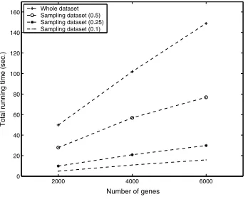
affects the efficiency of evaluating fitness of individuals. Fitness evaluation involves scanning the genes in the mi-croarray dataset and computing the Pearson’s Correlation Coefficient between the given gene and each other gene in a given subset of conditions. Thus, fitness evaluation is ex-pected to be linear with respect to the number of genes in the dataset. The two-stage progressive GA employs ran-dom sampling to enhance the speed. Different sampling ratios, 0.1, 0.25 and 0.5, are tested in this experiment. Here, the sampling ratio refers to as the ratio of the number of genes in the sample against the total number of genes in the whole dataset. Figure 3 shows the running time of the single-stage and two-stage progressive GA under varying number of genes. The results verify the linear behavior of the running time as we expect. Moreover, this result also demonstrates that two-stage GA, using sampling as an ef-fective means for speedup, is more efficient than the single-stage GA.
Effect of window size. The window size determines the
size of the search space for subsets of conditions within each window, which is in an exponential order of the win-dow size. This does not necessarily mean that the running time of our algorithm will be exponential with respect to the window size whatsoever. The actual running time is de-pended on how the search workload within each window is specified. More precisely, if we use the fixed number of generations and population size for each generation in the GA, i.e. fixed number of individualsto be evaluated in each window, then the total search workload for each win-dow will be the same. In this case, increase in winwin-dow size will consequently lead to a decrease, rather than an increase, in the number of window positions and therefore a drop of running time. Afixed ratio searchscheme, in contrast, per-forms a search workload that is proportional to the size of search space in this window. The time complexity now be-comes quadratic with respect to the window size. The run-ning time of these two search schemes are presented in Fig-ure 4. For each window position, the search workload with a fixed number of individuals is set to be 400 and that of a fixed ratio is 50% of the search space of the window.
6.2
Effectiveness Study
2000 4000 6000 0
20 40 60 80 100 120 140 160
Number of genes
Total running time (sec.)
Whole dataset Sampling dataset (0.5) Sampling dataset (0.25) Sampling dataset (0.1)
Figure 3. Running time for
single-stage and two-stage GA (with different sampling ratios) under varying number of genes
5 10 15 20
0 50 100 150 200 250 300
Window size
Running time (sec.)
[image:7.612.121.295.71.211.2]Fixed ratio Fixed number
Figure 4. Running time under varying window sizes
GA versus non-progressive scheme and the convergence of our method.
Fitness enhancement by using progressive GA. We first
study the contribution of progressive GA used in our method to enhancing the fitness of individuals, compared to the case when non-progressive GA is used. They primarily differ in that the progressive GA inherits the top-ranked in-dividuals obtained from the previous window position with appropriate modifications and bias is introduced in the ini-tial random population generation for the current window position, while the non-progressive GA evaluates each win-dow independently and the entire initial population for each window position is generated randomly. Figure 5 presents theaveragedfitness of top 10 individuals for each window position (from No. 1 to 26). The result demonstrates that the progressive GA outperforms non-progressive scheme in term of fitness in up to 88% of the window positions and fitness improvement by over 10% is observed at about 25% of the window positions. This result indicates that progres-sive GA is more capable of finding fitter individuals than the non-pregressive GA.
Convergence study. GA tends to produce an increasing
number of fitter individuals as evolution proceeds, referring to as the phenomenon of convergence. In this experiment, we investigate the convergence of our technique. Without losing generality, three window positions, the first, middle and last (1st,13thand26th), are picked up for this study.
For each generation, the number of individuals with rela-tive high fitness (> 0.7in this experiment) are counted. As we can see from Figure 6 that the number of individ-uals with high fitness is increased as the GA evolves, which indicates a good convergence of our method. In addition, the good individuals do not only appear in the last
gener-ation, though the overall convergence of the GA has been observed. A small number of good individuals have been observed in the earlier generations of the GA. This verifies the validity of keeping track of the top-ranked individuals in each generation of GA in our approach to prevent the loss of good individuals appearing in different, particularly the early, generations of the GA.
7
Conclusions
This paper investigates the problem of gene co-regulation discovery problem in DNA microarray data. Unlike most of the existing methods that find gene co-regulations utilizing clustering analysis, our approach aims to discover co-regulations from a single gene perspective. We are interested in finding the regulators of a given gene and the associated sets of experimental conditions in which such co-regulations occur. The basic idea of our approach is to first find the subsets of conditions in which the given geneg is most significantly co-regulated with other genes and the co-regulated genes ofg are reported by selecting from its nearest neighbors in these subsets of conditions.
0 5 10 15 20 25 0.45
0.5 0.55 0.6 0.65 0.7 0.75 0.8 0.85 0.9
Window positions
Fitness
Non−progressive Progressive
Figure 5. Fitness of
non-progressive and progressive
GA
0 2 4 6 8 10 12 14 16 18 20
0 1 2 3 4 5 6 7 8
Generation ID
Number of individual having high fitness values
[image:8.612.124.296.73.212.2]window position 1 window position 13 window position 26
Figure 6. Number of individu-als having high fitness values in three window positions
is effcient and effective in discovering gene-specific local co-regulations from gene expression data.
Acknowledgement
The authors would like to thank Dr. Malcolm I. Heywood and Dr. Christian Blouin, both from Faculty of Computer Science at Dalhousie University, for their useful suggestions on the draft of this paper. This research work is supported in part by research grant of Natural Sciences and Engineering Research Council of Canada (Grant No.: 312423).
References
[1] C. C. Aggarwal, J. B Orlin and R. P Tai. Optimized Crossover for the Independent Set Problem.Operational Re-search45(2):226-234, 1997.
[2] C. C. Aggarwal and P.S. Yu. An Effective and Efficient Algo-rithm for High-dimensional Outlier Detection.VLDB Jour-nal, 14, pp 211-221, 2005.
[3] S. Bhattcharrya. Direct Marketing response Meodels Using Genetic Algorithms.KDD’98, pp 144-148, 1998.
[4] Y. Cheng and G.M. Church, Biclustering of Expression Data. InProc. International Conference on Intelligent Systems for Molecular Biology (ISMB), vol. 8, pp. 93-103, 2000. [5] G. Getz, E. Levine, and E. Domany, Coupled Two-Way
Clus-tering Analysis of Gene Microarray Data, inProc. Natioal Academy of Science, vol. 97, no. 22, pp. 12079-12084, 2000. [6] G. H Golub and C. F. Van Loan.Matrix Computations, Johns
Hopkins University Press, 1983.
[7] J. Holland.Adaption in Natural and Artificial Systems. MIT Press, Cambridge, 1992.
[8] L. Ji and K. L. Tan. Identifying Time-Lagged Gene Clusters on Gene Expression Data.Bioinformatics, Vol. 21, No. 4, pp. 509-516, 2005.
[9] R. A. Johnson and D. W. Wichern.Applied Multivariate Sta-tistical Analysis, Prentice Hall International, USA, 1998.
[10] T. Kohonen. Self-Organization Maps. Springer-Verlag, Berlin Heidelberg, 1995.
[11] A. T. Kwon, H. H. Hoos, and R. Ng. Inference of transcrip-tional regulation relationships from gene expression data.
Bioinformatics, 19, 905-912, 2003.
[12] C. A. Orengo, D. T. Jones and J. M. Thornton. Bioinformat-ics. Genes, proteins and Computers. BIOS Scientific Pub-lishers ltd, Oxford, UK, 2003.
[13] T. Speed, J. Fridlyand, Y. H. Yang and S. Dudoit. Dis-crimination and clustering with microarray gene expression data.2001 Spring Meeting of International Biometric Society Eastern North American Region (ENAR’01), Charlotte NC, 2001.
[14] R. Tibshirani, T. Hastie, M. Eisen, D. Ross, D. Bostein and P. Brown. Clustering Methods for the Analysis of DNA Mi-croarray Data.Technical Report, Stanford, 1999.
[15] J. Yang, W. Wang, H. Wang, and P.S. Yu,δ-Cluster: Captur-ing Subspace Correlation in a Large Data Set. InProc. 18th International Conference on Data Engineering (ICDE’02), pp. 517-528, 2002.
[16] Y. Zhang, H. Zha, J. Z. Wang, C. Chu. Gene Co-regulation vs. Co-expression8th