Nodal integration finite element techniques for analysis of piezoelectric solids

CSM2008

The International Conference on Computational Solid Mechanics November, 27 –30, 2008

Hochiminh City, Vietnam

Nodal integration finite element techniques for analysis of piezoelectric

solids

H. Nguyen-Van1, 2_{, Thong Le}2_{, N. Mai-Duy}1 _{and T. Tran-Cong}1

¹ Computational Engineering & Science Research Centre (CESRC) Faculty of Engineering and Surveying, University of Southern Queensland, Australia.

2

Faculty of Civil Engineering, University of Architecture, Ho Chi Minh City, Vietnam.

Abstract

A stabilized conforming nodal integration (SCNI) method is presented to formulate two efficient smoothing piezoelectric elements for static analysis of planar piezoelectric structures with quadrilateral mesh. The approximations of mechanical strains and electric potential fields are normalized by the smoothing constant function of the SCNI technique over each smoothing cell. This method allows field gradients to be directly computed from interpolating shape functions using boundary integrations along each edge of the smoothing element. The boundary integration will contribute to the preservation of high accuracy of the method even when elements are extremely distorted, for example, a concave quadrilateral. No mapping or coordinate transformation and derivatives of shape functions are necessary so that the original meshes with badly shaped elements can be used. The present elements do not introduce any additional degrees of freedom and are easy to implement into an existing finite element method (FEM). Numerical examples and comparative studies with analytic solutions are presented to demonstrate the simplicity, efficiency and accuracy of the elements.

Key Words: Piezoelectric structures, Nodal integration finite element method, Electro-mechanics.

1. Introduction

Piezoelectric materials have many applications in various modern engineering fields such as smart structures, mechatronics, or micro-electromechanical system (MEMS) technology. It is evident that they have attracted significant attention of researchers. Great progress have been made over past decades towards better understanding of electromechanical coupling behaviour of piezoelectric materials using analytic/numerical methods and experimental models. Since the work of Allik and Hughes (1970) using FEM to analyze the vibration of piezoelectric media, the literature on piezoelectric FEM has been developed extensively and is too large to list here. More details and reviews on the development of the FEM for piezoelectric materials and smart structures can be found in Mackerle (2003).

application of the SCNI in the FEM has been further developed for the analysis of coupling between mechanical and electrical behaviours of 2D piezoelectricity structures by Nguyen-Van et al. (2008a, b, c). A family of simple, accurate and efficient planar low-order piezoelectric elements have been successfully developed by the present authors.

In this paper, two types of the developed elements are introduced and summarized for static analysis of piezoelectric solids.

2. Review of finite element formulations for 2D piezoelectric problems

The mechanical constitutive relation for 2D piezoelectric materials can be expressed in the e–form as follows.

E e

ε

c

σ= E − T , (1)

gE eε

D= + , (2)

where cE, is the plane elastic stiffness matrix, e is the plane piezoelectric matrix and g is the plane

dielectric constant matrix.

Equations (1)–(2) can be rewritten in the explicit form in the x–z plane as

11 13 31

13 33 33

55 15

0 0

0 0

0 0 0

x x

x

z z

z

xz xz

c c e

E

c c e

E c e σ ε σ ε τ γ                   = −          _{ }                

, (3)

15 11

31 33 33

0 0 0

0 0 x x x z z z xz e g D E

e e g

D E ε ε γ             =_{ } +_{ }   _{ }      _{ }     

. (4)

The finite element approximation solution for 2D piezoelectric problems using the standard linear element can be expressed as

1

np i

u i u

i=

=

∑

u N q N q, (5)

1 np i i i φ φ =

=

∑

φ φ

φ φ

φ φ

φ φ , (6)

where np is the number of nodes of an element; q, ϕϕϕϕ are the nodal displacement and nodal electric potential vectors and Nu, Nφ are shape function matrices.

The corresponding approximation of the linear strain εεεε and electric field E are

s u

= ∇ =

ε u B q, (7)

φ

= −∇ = −

E φφφφ B φ, (8)

where , , , , 0 0 i x i

u i z

i z i x N N N N     =     

B , ,

, i x i i z N N φ   =   

B . (9)

0 0 0 e e e uu u uu e e u φ φ φφ             + =                   _{ } K K

q q F

M

φ K K φ Q

&&

&& , (10)

in which

e T

uu=

∫

M N N , (11)

e T

uu u E ud

Ω

=

∫

K B c B , (12)

e T T

uφ u φd

Ω

=

∫

K B e B , (13)

e T

d

φφ φ φ

Ω

= −

∫

K B gB , (14)

T T

u d u d

Ω Ω

=

∫

∫

F N f N t ,

q

T

d

φ Γ

=

∫

Q N q . (15)

For static analysis (q&&=0), Equation (10) is reduced to

e e uu u e e u φ φ φφ  _{    }  _{   =}        

K K q F

φ Q

K K . (16)

3. Nodal integration techniques for piezoelectric finite element method

In the SCNI technique, the strain (ε%) and the electric (E%) field used to evaluate the stiffness matrix is computed by a weighted average of the standard strain and electric field of the finite element method. In particular, at an arbitrary point xk in a smoothing element domain k

Ω , they are approximated as follows.

( ) _k ( ) ( )

k k k k

d

Ω

=

∫

ε% x ε x x x , (17)

( ) _k ( ) ( )

k k k k

d

Ω

=

∫

E x% E x x x , (18)

where k

Φ is a smoothing function that is here chosen as a constant function

1/ ( ) 0 k k k k k A

 _{∈ Ω}

 Φ − =

∉ Ω  x x x x (19)

in which

∫

ΩΩ

= d_k

Ak is the area of the smoothing cell k

Ω .

Two schemes are proposed to transform original finite elements into smoothing domains k

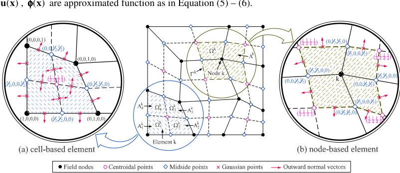
Ω (smoothing elements) in which the smoothing operation of the SCNI is performed. The first scheme forms the so-called cell-based element approach and the second the node-based element approach. The two approaches are illustrated in detail in Figure 1.

Substituting Φk into Equation (17) – (18) and applying the divergence theorem, we obtain a smoothed strain and smoothed electric field in the domain k

Ω as

1 1

( ) _k ( ) _k ( )

k k k

s u

k d k d

A Ω A Γ

=

∫

∫

ε% x u x n u x , (20)

1 1

( ) _k ( ) _k ( )

k k k

k d k d

A Ω A Γ φ

= −

∫

∫

where k u

n and k

φ

n are matrices associated with unit outward normal to the boundary k

Γ , 0 0 k x k k u z k k z x n n n n     =        n , k x k k z n n φ   =     

n , (22)

and u x( ), φφφφ( )x are approximated function as in Equation (5) – (6).

Figure 1. Details of smoothing elements: (a) Cell-based element: each element is divided into 4 smoothing cells, (b) Node-based element: each smoothing cell associated with a node is built by connecting midside

points with centroidal points of original elements surrounding the node.

By introducing the finite element approximation of u and φφφφ, Equation (20)–(21) can be transformed in the matrix form as follows.

1

( ) ( )

nk

k k i k

u i

i=

=

∑

ε% x B x q% , (23)

1

( ) ( )

nk

k k i k

i i

φ

=

= −

∑

E x% B x% φφφφ, (24)

where nk is the number of nodes connecting directly to node k (node-based element approach) or the number of subcells (cell-based element approach),

0 1

( ) _k 0

k i x

i k k

u k i z

k k

i z i x

N n

N n d A

N n N n

Γ

 

 

= _{ } Γ

 

 

∫

B x% , (25)

1

( ) k

k

i k i x

k k

i z N x

d

A N x

φ _Γ

 

=   Γ

 

∫

B x% . (26)

When bilinear quadrilateral elements are used for modelling, a linear completed displacement field along the boundary k

Γ is guaranteed. Therefore, one Gaussian point is sufficient for accurate boundary integration along each line segment k

i

Γ of the contour k

Γ of the domian k

Ω , and Equations (25) – (26) can be evaluated as

1

( ) 0

1

0 ( )

( ) ( )

G k

i b x

nb

i G k k

u k i b z b

b G k G k

i b z i b x

N n

N n l

A

N n N n

=     =        

∑

1

( ) 1

( )

G k

nb

i b x

i k

b

k G k

b i b z

N n

l

A N n

φ

=

 

=  

 

 

∑

B

x

% _{, (28)}

where nb is the total number of the line segments of the contour k

Γ , G b

x is the midpoint (Gauss point) of each line segment k

b

Γ , whose length and outward unit normal are k b

l and _nk_{, respectively.}

Finally, the element stiffness matrices in Equations (12) – (14) can be rewritten as follows.

1

nk

k iT i k

uu u E u

i

A

=

=

∑

K% B c B% % (29)

1

nk

k iT T i k

u u

i

A

φ φ

=

=

∑

K% B e B% % (30)

1

nk

k iT T i k

i

A

φφ φ φ

=

= −

∑

K% B g B% % (31)

4. Numerical examples

In this section, two examples are employed to demonstrate and assess the performance of two smoothing elements as applied to the linear static analysis of two-dimensional piezoelectric structures. The node-based smoothing piezoelectric element is denoted as NSPE-Q4 and the cell-based one as SPE-Q4.

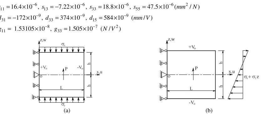
A piezoelectric (PZT-5) strip, polarized in the z-direction, under a combined loading of pressure and applied voltage is analyzed (Figure 2). Two types of combined loads corresponding to shear and bending behaviour are considered, respectively. The material PZT-5 is used for the problems and its properties are

6 6 6 6 2

11 13 33 55

9 9 9

31 33 15

8 7 2

11 33

16.4 10 , 7.22 10 , 18.8 10 , 47.5 10 ( / )

172 10 , 374 10 , 584 10 ( / ) 1.53105 10 , 1.505 10 ( / )

s s s s mm N

d d d mm V

g g N V

− − − −

− − −

− −

= × = − × = × = ×

= − × = × = ×

= × = ×

(a) (b)

Figure 2. A piezo-strip under different combined loads: (a)shear deformation and (b) bending deformation.

The boundary conditions for the piezo-strip in shear are

, 0 0

0

( , ) 0, ( , ) , ( , ) 0, ( , ) 0, ( , ,

( , ) 0, (0, ) , (0, ) 0, (0, 0) 0.

z z xz xz

z

x h x h L z x h L yz V

L z z V u z w

σ σ τ τ

σ

φ ± = ± = = ± = φ = −

= φ = + = =

0 , 0 1 ,

( , ) , ( , ) 0, ( , ) 0, ( , ) 0, ( , ) ,

( , ) 0, (0, ) 0, (0, ) 0, (0, 0) 0.

z xz x x

xz x

x h V x h x h L z L z z

L z z u z w

σ τ σ σ σ

τ

φ ± = ± ± = ± = φ = = +

= φ = = =

The analytic solutions for these problems can be found in Gaudnzi and Bathe (1995). In the calculation, we set L= 2h= 1 mm, σo= -5 N/mm2, σ1= 20 N/mm2 and V0= 1000V.

Two meshes, one with 8×8 uniform elements and the other with 8×8 distorted elements, are considered in this analysis as shown in Figure 3.

0 0.2 0.4 0.6 0.8 1 −0.5

−0.4 −0.3 −0.2 −0.1 0 0.1 0.2 0.3 0.4 0.5

x

y

0 0.2 0.4 0.6 0.8 1 −0.5

−0.4 −0.3 −0.2 −0.1 0 0.1 0.2 0.3 0.4 0.5

x

(a) (b)

Figure 3. Typical meshes of a piezo-strip: (a) regular elements and (b) irregular elements.

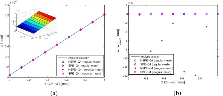
All the numerical results of the piezo-strip in shear are compared with corresponding analytic solutions and plotted together in Figures 4 – 6.

0 0.2 0.4 0.6 0.8 1 −1.5

−1 −0.5 0 0.5

1x 10

−6

x (z= −h) [mm]

u−u

exact

[mm]

Analytic solution NSPE−Q4 (regular mesh) SPE−Q4 (regular mesh) NSPE−Q4 (irregular mesh) SPE−Q4 (irregular mesh)

(a) (b)

Figure 4. A piezo-strip in shear: (a) u-displacement distribution, (b) u-displacement error.

0 0.2 0.4 0.6 0.8 1 −14

−12 −10 −8 −6 −4 −2 0 2x 10

−7

x (z= −h) [mm]

w−w

exact

[mm]

Analytic solution NSPE−Q4 (regular mesh) SPE−Q4 (regular mesh) NSPE−Q4 (irregular mesh) SPE−Q4 (irregular mesh)

(a) (b)

0 0.2 0.4 0.6 0.8 1 −12

−10 −8 −6 −4 −2 0 2 4 6x 10

−23

x (z= −h) [mm]

φ

−

φexact

[GV]

Analytic solution NSPE−Q4 (regular mesh) SPE−Q4 (regular mesh) NSPE−Q4 (irregular mesh) SPE−Q4 (irregular mesh)

(a) (b)

Figure 6. A piezo-strip in shear: (a) φ-electric potential, (b) φ-electric potential error.

It can be seen that all the computed displacements and electric potentials for both meshes and for both elements are in good agreement with analytic solutions.

For a uniform mesh, it is observed that the performance of SPE-Q4 element and NSPE-Q4 element achieves similar predictions. However, for the distorted mesh, the accuracy of SPE-Q4 for displacements is better than that of the NSPE-4 as can be seen from Figure 4b–5b.

0 0.2 0.4 0.6 0.8 1

−4 −3 −2 −1 0 1 2 3

4x 10

−6

z (x= L)[mm]

u−u

exact

[mm]

Analytic solution NSPE−Q4 (regular mesh) SPE−Q4 (regular mesh) NSPE−Q4 (irregular mesh) SPE−Q4 (irregular mesh)

(a) (b)

Figure 7. A piezo-strip in bending: (a) u-displacement distribution, (b) u-displacement error.

0 0.2 0.4 0.6 0.8 1 −8

−6 −4 −2 0 2 4x 10

−6

x (z= −h) [mm]

w−w

exact

[mm]

Analytic solution NSPE−Q4 (regular mesh) SPE−Q4 (regular mesh) NSPE−Q4 (irregular mesh) SPE−Q4 (irregular mesh)

(a) (b)

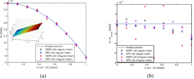
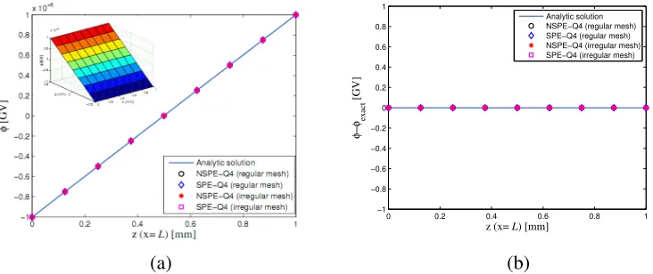
The numerical results for the piezo-strip in bending are illustrated in Figure 7–9. As can be seen, both computed displacements and electric potential match well the exact solutions for SPE-Q4 element as well as NSPE-Q4 element.

Once again, the SPE-Q4 element demonstrates better performance with respect to displacement fields than that of the NSPE-Q4 for the distorted mesh. For the uniform mesh, both elements perform nearly equally well.

0 0.2 0.4 0.6 0.8 1 −1

−0.8 −0.6 −0.4 −0.2 0 0.2 0.4 0.6 0.8 1

z (x= L) [mm]

φ

−

φexact

[GV]

Analytic solution NSPE−Q4 (regular mesh) SPE−Q4 (regular mesh) NSPE−Q4 (irregular mesh) SPE−Q4 (irregular mesh)

(a) (b)

Figure 9. A piezo-strip in bending: (a) φ-electric potential, (b) φ-electric potential error.

5. Conclusions

Two efficient piezoelectric elements based on nodal integration finite element techniques are developed and presented for linear static analysis of 2D piezoelectric solids. Numerical solutions are verified by excellent agreement with analytic solutions. Particularly, the present method can yield accurate results even with extremely distorted meshes.

6. References

Allik, H., Hughes, T. (1970). Finite element method for piezoelectric vibration. International Journal for Numerical Methods in Engineering, 2, pp. 151–157.

Chen, J., Wu, C., and You, Y. (2001) A stabilized conforming nodal integration for Galerkin meshfree method. International Journal for Numerical Methods in Engineering, 50, pp. 435–466.

Dai, K. Y. and Liu, G. R. (2007a). Free and forced vibration analysis using the smoothed finite element method (SFEM). Journal of Sound and Vibration, 301 (3–5), pp. 803–820.

Dai, K. Y., Liu, G. R., and Nguyen T. T. (2007b). An n-sided polygonal smoothed finite element method (nSFEM) for solid mechanics. Finite Elements in Analysis and Design, 43(11-12), pp. 847-860.

Gaudnzi, P., and Bathe, K. J. (1995). An iterative finite element procedure for the analysis of piezoelectric continua. Journal of Intelligent Material System Structures, 6, pp. 266–273.

Lim, C. W., and Lau, C. W. H. (2005). A new two-dimensional model for electro-mechanical response of thick laminated piezoelectric actuator. International Journal of Solids and Structures, 42, pp. 5589–5611.

Liu, G. R., Dai, K. Y., Lim, K. M., and Gu, Y. T. (2002). A point interpolation mesh free method for static and frequency analysis of two-dimensional piezoelectric structures. Computational Mechanics, 29, pp. 510–519.

Liu, G. R., Dai, K. Y., and Nguyen, T. T. (2007a). A smoothed finite element method for mechanics problems. Computational Mechanics, 39(6), pp. 859–877.

Liu, G. R., Nguyen, T. T., Dai, K. Y., and Lam, K. Y. (2007b). Theoretical aspects of the smoothed finite element method (SFEM). International Journal for Numerical Methods in Engineering, 71, pp. 902–930.

Mackerle, J. (2003). Smart materials and structures – an finite element approach - an addendum: a bibliography (1997-2002). Modelling and Simulation in Materials Science and Engineering, 11, pp. 707–744.

Nguyen-Van, H., Mai-Duy, N., and Tran-Cong, T. (2008a). A smoothed four-node piezoelectric element for analysis of two-dimensional smart structures. CMES: Computer Modeling in Engineering & Sciences, 23(2), pp. 209-222.

Nguyen-Van, H., Mai-Duy, N., and Tran-Cong, T. (2008b). Analysis of piezoelectric solids with an efficient node-based smoothing element. The 8th World Congress on Computational Mechanics (WCCM8), June 30 –July 5, 2008, Venice, Italy.

Nguyen-Van, H., Mai-Duy, N., and Tran-Cong, T. (2008c). A node-based element for analysis of planar piezoelectric structures. CMES: Computer Modeling in Engineering & Sciences (accepted)

Ohs, R. R., and Aluru, N. R. (2001). Meshless analysis of piezoelectric devices. Computational Mechanics, 27, pp. 23–36.