Solving high-order partial differential equations with indirect radial basis function networks

Solving High-Order Partial Differential Equations

with Indirect Radial Basis Function Networks

N. Mai-Duy

and R.I. Tanner

School of Aerospace, Mechanical and Mechatronic Engineering,

The University of Sydney, NSW 2006, Australia

Submitted to

Int. J. Numer. Meth. Engng

, 21st June 2004; revised

25 November 2004

SUMMARY

This paper reports a new numerical method based on radial basis function

net-works (RBFNs) for solving high-order partial differential equations (PDEs). The

variables and their derivatives in the governing equations are represented by

inte-grated RBFNs. The use of the integration process in constructing neural networks

allows the straightforward implementation of multiple boundary conditions and the

accurate approximation of high-order derivatives. The proposed RBFN method is

verified successfully through the solution of thin-plate bending and viscous flow

problems which are governed by biharmonic equations. For thermally driven cavity

flows, the solutions are obtained up to a high Rayleigh number of 107.

KEY WORDS: radial basis functions; approximation; multiple boundary conditions;

1

INTRODUCTION

Neural networks have found application in many disciplines: neurosciences,

math-ematics, statistics, physics, computer science and engineering [1]. The concept of

using radial basis function networks (RBFNs) to solve partial differential equations

(PDEs) was introduced by Kansa in 1990 [2]. Since then it has received much

atten-tion from the science and engineering communities. The construcatten-tion of networks

can be based on a differentiation process (the direct RBFN approach - DRBFNs) [2]

or based on an integration process (the indirect RBFN approach - IRBFNs) [3]. For

a typical RBFN-based numerical method, each dependent variable and its

deriva-tives are represented by DRBFNs/IRBFNs. The governing differential equations

together with boundary conditions are then discretized by point collocation. Most

RBF publications were concerned with the solution of second-order PDEs, e.g.,

[4-9]. Recently, the IRBFN method has been developed for the solution of high-order

ordinary differential equations (ODEs) without prior conversions into the

equiva-lent systems of first-order ODEs [10]. In this paper, the unsymmetric indirect RBF

collocation method is extended to solve high-order PDEs directly.

Consider problems governed by multi-harmonic equations, such as thin-plate

bend-ing and Stokes flow problems involvbend-ing biharmonic equations. To solve these

prob-lems, new variables are usually introduced in order to transform the multi-harmonic

equations into the coupled sets of harmonic equations from which the conventional

low-order methods of discretization such as the boundary element methods (BEMs),

finite difference methods (FDMs) or finite element methods (FEMs) can be applied

for obtaining a numerical solution. However, the drawbacks of this transformation

are that it produces large system matrices as well as one usually needs to derive

the computational boundary conditions for new variables. All of these difficulties

multi-harmonic equations directly. In addition, the high-order methods are known

to have the capability to achieve accurate results using relatively low numbers of

degrees of freedom (DOF) or to allow the savings in computational effort and virtual

storage for a given accuracy [11].

In solving high-order PDEs in a direct manner, special attention needs to be paid

to the two important issues, namely the implementation of multiple boundary

con-ditions and the approximation of high-order derivatives. To properly implement

the multiple boundary conditions, there are a number of techniques available in

the literature, e.g., the δ-technique [12], the modified weighting matrix approach

[13], the approach of directly substituting the boundary conditions into the discrete

governing equations [14], the general approach [15] and the generalized differential

quadrature rule (GDQR) technique [16]. The basic ideas of these techniques are to

try adding “extra boundary points” to the original set of data points so that each

boundary point has only one condition (the δ-technique), reducing the number of

data points used for discretizing the governing equations in an appropriate

man-ner (the direct substitution technique) and employing the same number of unknown

variables as that of the conditions at a point (the GDQR technique), in order to form

a square system matrix. More detailed discussions can be found in [16,17]. In the

context of the numerical solution of differential equations, high-order derivatives are

undesirable in general because they can introduce large approximation error. The

use of higher-order conventional Lagrange polynomials does not guarantee to yield

a better quality (smoothness) of approximation [18].

The two important issues mentioned above can be treated effectively here by using

integrated RBFNs. In the present unsymmetric indirect RBF collocation approach,

the construction of neural networks representing the variable and its derivatives is

based on integration. The governing equations and boundary conditions are

to the presence of integration constants is brought into balance with the increase

of rows due to the discretization of multiple boundary conditions, and hence it can

lead to a square system matrix whatever the order of PDEs. On the other hand,

the integration process appears to be suitable for the approximation of high-order

derivatives. It can be argued as follows. Due to the lack of theory, it is very

dif-ficult to choose RBFN parameters, such as RBF widths, properly. Consequently,

some oscillation can be induced between the nodal function values when using the

RBFN interpolation scheme. This behaviour has no relation at all to that of the

true function. In practice, the oscillation has been often observed in regions near the

boundaries. It can be seen that by differentiating RBFNs, the spurious oscillations

will be strongly magnified with an increase in order of derivatives (the slope of the

curve). However, it is expected that the process of integrating RBFNs (the area

under curve) can suppress “noise”, thereby resulting in smoother approximating

derivatives.

The present unsymmetric IRBFN collocation method will be verified with the

so-lution of thin-plate bending and viscous flow problems that are governed by

bi-harmonic equations. In the simulation of natural convection flows, the resultant

matrices become much larger due to the increased number of the field variables and

the requirement of dense data densities for the simulations at high Rayleigh

num-bers. To keep the system matrix size comparable to that associated with the DRBFN

approach, the multiple spaces of IRBFN weights for each variable are converted into

the single space of nodal variable values.

The remainder of the paper is organized as follows. In section 2, RBFNs and their

two direct and indirect approaches for the approximation of a function and its

deriva-tives are reviewed. Section 3 presents IRBFNs for solving high-order PDEs without

prior conversions into the equivalent systems of low-order PDEs. In sections 4 and

problems and thermally driven cavity flows that are governed by biharmonic

equa-tions. Section 6 gives some concluding remarks. Finally, the analytic forms of new

basis functions obtained from integrating RBFs are given in the appendix.

2

RADIAL BASIS FUNCTION NETWORKS

RBFNs allow a conversion of a function from low-dimensional space (e.g., 1D-3D)

to high-dimensional space in which the function will be expressed as a linear

com-bination of RBFs [1]

y(x)≈f(x) =

m

i=1

w(i)g(i)(x), (1)

where y and f are the exact and approximate functions, respectively, superscripts

denote the elements of a set of neurons,xthe input vector, mthe number of RBFs,

{w(i)}m_i=1 the set of network weights to be found, and{g(i)(x)}m_i=1 the set of RBFs.

According to Micchelli’s theorem, there is a large class of radial basis functions, e.g.,

multiquadrics, inverse multiquadrics and Gaussian functions, whose design matrices

(interpolation matrices, coefficient matrices) obtained from (1) are always

invert-ible, provided that the data points are distinct. This is all that is required for the

non-singularity of the design matrix, whatever the number of data points and the

dimension of the problem [1]. On the other hand, the Cover’s theorem, which can

be stated as follow “the higher the dimension of hidden space, the more accurate the

approximation will be” [1], indicates the property of “mesh convergence” of RBFNs.

Furthermore, it has been proved that RBFNs are capable of representing any

contin-uous function to a prescribed degree of accuracy (universal approximation theorem)

[19]. These important theorems can be seen to provide the theoretical basis for the

Since multiquadrics (MQ) are ranked as the most accurate among RBFs [20] and

possess exponential convergence with the refinement of spatial discretization [21,22],

this study will employ these basis functions whose form is

g(i)(x) =

(x−c(i))T(x−c(i)) +a(i)2, (2)

wherec(i)anda(i)are the centre and width of theith MQ basis function, respectively, and superscript T denotes the transpose of a vector. To make the training process

simple, the centres and widths of RBFs are chosen in advance. For the former, the

set of centres is chosen to be the same as the set of collocation points, while for the

latter, the following relation is used

a(i) =βd(i), (3)

whereβ is a positive scalar, andd(i)is the minimum of distances from theith center to its neighbours. Relation (3) allows the RBF widtha to be broader in the area of

lower data densities and narrower in the area of higher data densities. The network

weights are then found by minimizing the sum of squares of the difference between

actual and required outputs.

2.1

Direct approach

In the direct RBFN (DRBFN) approach, the RBFN (1) is utilized to represent the

(1) as

y(x) ≈ f(x) =

m

i=1

w(i)g(i)(x), (4)

∂yk(x)

∂xk_j ≈

∂kf(x)

∂xk_j =

∂km_i=1w(i)g(i)(x)

∂xk_j =

m

i=1

w(i)h[_[k_x](i)

j] (x), (5)

where subscripts j denote the scalar components of a vector, and

h[_[k_x](i)

j] (x)

_m

i=1 = ∂

k_g(i)_(x)/∂xk j

m

i=1 the set of newly derived basis functions in the

approximation of the kth-order derivative of a function y with respect to the x_j

variable.

2.2

Indirect approach

In the indirect (IRBFN) approach, RBFNs (1) are used to represent the

highest-order derivatives of a function y, e.g., ∂ky/∂xk_j. Lower-order derivatives and the

function itself are then obtained by integrating those RBFNs as

∂ky(x)

∂xk_j ≈

∂kf(x)

∂xk_j =

m

i=1

w(_[xi)

j]g

(i)_{(x), (6)}

∂k−1y(x)

∂xk_j−1 ≈

∂k−1f(x)

∂xk_j−1 =

m+q1

i=1

w(_[xi)

j]H

[k−1](i)

[xj] (x), (7)

· · · ·

y(x) ≈ f_[xj](x) =

m+qk i=1

w(_[xi)

j]H

[0](i)

[xj] (x), (8)

where subscripts [x_j] denote the quantities associated with the process of integration

in thex_j direction; q₁,· · · , q_k the numbers of nodal constants arising from the inte-gration process (inteinte-gration constants are directly captured here) (q₂ = 2q₁,· · · , q_k =

kq₁); and

H_[[_xk−1](i)

j] =

g(i)dx_j, H_[[_xk−2](i)

j] =

H[k−1](i)dx_j,· · · , H_[[0](_x i)

j] =

(k −2)th-order derivative, · · ·, the original function y, respectively. Note that for

convenience of notation, the integration constants (unknowns) and their associated

basis functions (known polynomials) are also denoted by the notations w(i) and

H[.](i)(x), respectively, but withi > m.

The evaluation of (6)-(8) at a set of collocation points{x(i)}n_i=1 yields the following systems of equations

f_[[_xk]

j](x) = G(x)w[xj], (9)

f_[[_xk−1]

j] (x) = H

[k−1]

[xj] (x)w[xj], (10)

· · · ·

f_[xj](x) = H[0]_[x

j](x)w[xj], (11)

where G_[xj],H[_[k_x−1]

j] ,· · · ,H

[0]

[xj] are the network-design-matrices associated with the approximation of thekth-order derivative, (k−1)th-order derivative,· · ·, the original

function with respect to the x_j variable, respectively; w_[xj] = {w(_[xi)

j]} m+qk

i=1 the set

of network weights in the x_j direction to be found; f_[xj] = {f_[xj](x(i))}n_i=1; f_[[1]_x j] =

{∂f_∂x(x(_ji))}n

i=1; andf[[xkj]]={

∂k_f(x(i)₎

∂xk

j }

n

i=1. For the purpose of computation, the matrices

G_[xj],H[_[k_x−1]

j] ,· · · ,H

[1]

[xj] will be augmented using zero-submatrices so that they have the same size as the matrix H[0]_[x

j]. In the approximation of a function and its derivatives, the IRBFN weight vectorsw_[xj] with j ={1,2,· · · } can be determined by making use of the functional networks (11).

For convenience of presentation, the following discussions are restricted to

bihar-monic boundary value problems. However, they can be extended straightforwardly

to multi-harmonic ones, and furthermore, all of the advantageous features found in

the case of biharmonic problems can be preserved. The cross derivative∂f4(x)/∂x2_i∂x2_j

can be computed by using the relevant network-design-matrices associated with the

theoretically, due to numerical error, it will be better to take the average of the two

equivalent representations

∂4f ∂x2_i∂x2_j =

1 2

∂2 ∂x2_i

∂2f ∂x2_j

+ ∂

2

∂x2_j

∂2f ∂x2_i

, (12)

or in the matrix form

f_,iijj = 1

2

H[2]_[x i](H

[0] [xi])

−1_H[2]

[xj]w[xj]+

H[2]_[x j](H

[0] [xj])

−1_H[2] [xi]w[xi]

. (13)

Expressions off and its derivatives at point x₀ in terms of network weightsw_[xj] =

{w_[(_xi)

j]} m+q4

i=1 can be given by

f(x₀) = 1

N

N

j=1

H_[[0](1)_x

j] (x0),· · · , H

[0](m+1)

[xj] (x0),· · · , H

[0](m+q1+1)

[xj] (x0),· · ·

w_[xj]

,

(14)

∂f2(x₀)

∂x2_j =

H_[[2](1)_x

j] (x0),· · · , H

[2](m+1)

[xj] (x0),· · · , H

[2](m+q1+1)

[xj] (x0),· · ·

w_[xj], (15)

∂4f(x₀)

∂x4_j =

g_[(1)_x

j](x0),· · ·,0,· · · ,0,· · ·

w_[xj], (16)

∂4f(x₀)

∂x2_i∂x2_j =

1 2(

H_[[2](1)_x

i] (x0),· · · , H

[2](m+1)

[xi] (x0),· · ·

(H[0]_[x i])

−1_H[2] [xj]w[xj]

+

H_[[2](1)_x

j] (x0),· · · , H

[2](m+1)

[xj] (x0),· · ·

(H[0]_[x j])

−1_H[2] [xi]w[xi]

), (17)

where N is the dimension of the problem. In (14), due to numerical errors, the

3

IRBFNs for solving high-order PDEs

Indirect RBFNs are employed to represent the solution of high-order PDEs via a

point collocation mechanism. The governing equations are solved without splitting

them into the equivalent systems of low-order PDEs. New constants arising from

the integration process are used for the treatment of multiple boundary conditions.

In constructing system/interpolation matrices, the increase of rows due to the

dis-cretization of multiple boundary conditions is brought into balance with the increase

of columns due to the presence of integration constants, and hence it can lead to a

square system of equations whatever the order of DEs.

The detailed implementation of IRBFNs for the solution of high-order ODEs was

reported previously in [10]. In present work that deals with high-order PDEs, two

versions of indirect RBFNs are employed. The first version uses the IRBFN

for-mulation directly in terms of network weights, while in the second version, the

formulation is expressed in terms of nodal variable values. The following is

con-cerned with biharmonic equations governing thin-plate problems and viscous flows.

However, the formulations can be extended to solve multi-harmonic equations in a

4

THIN-PLATE PROBLEMS

4.1

Governing equations

In this section, the deflection and free vibration of thin rectangular plates are

con-sidered. The governing equations can be written as

∇4_{v = F(x), (deflection) (18)}

∇4_{v = Ω}2_{v, (free vibration) (19)}

and the boundary conditions are given by

v = 0, ∂v

∂n = 0 for a clamped edge, (20)

v = 0, ∂

2_v

∂n2 = 0 for a simply supported edge, (21)

wherexis the position vector of a point in the domain of interest,vthe deflection/the

mode shape function, Ω the frequency, F the forcing term, and n the direction

normal to the edge.

4.2

IRBFN formulation

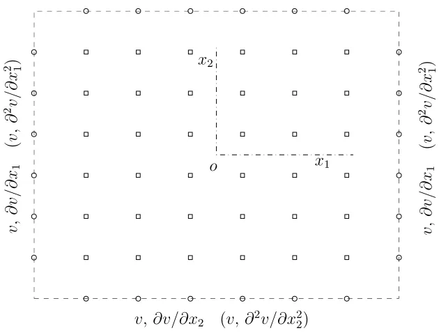
The rectangular domain of interest is discretized as shown in Figure 1. It is different

from the 1D-IRBFN analysis that there exist two RBF networks representing the

variable v here. These functional networks need to be enforced to be identical,

resulting in a constraint equation v_[x1](x) = v_[x2](x). The IRBFN formulation can be written as

where SSE₁, SSE₂ and SSE₃ are the sums of squared errors which are employed to ensure that IRBFNs satisfy the governing equation, the identical

representa-tions of the original function (i.e., v_[x1](x) = v_[x2](x)), and the boundary condi-tions, respectively. Let nip and nbp_j denote the number of interior points and

the number of boundary points on the plate edge normal to the x_j direction,

re-spectively. It can be seen that the direct matrix obtained from (22) will have the

number of rows as [(nip+ 2nbp₁ + 2nbp₂) + (nip) + (4nbp₁ + 4nbp₂)] that corre-sponds to SSE₁, SSE₂ and SSE₃, respectively, and the number of columns as [(nip + 2nbp₁ + 4nbp₁) + (nip+ 2nbp₂ + 4nbp₂)] that corresponds to the network weights in the x₁- and x₂- directions, respectively. Hence, the formulation (22) directly results in a square system matrix.

4.3

Numerical examples

A number of examples are presented in this section to demonstrate the effectiveness

of the present method. In all following test cases, the width of the ith RBF (a(i)) is simply chosen to be the minimum distance from the ith centre to neighbouring

centres (β = 1). The accuracy of numerical solution produced by an approximation

scheme can be measured via the norm of relative errors of the solution as follows

N_e=

_n

i=1[ve(x(i))−v(x(i))]2 n

i=1ve(x(i))2

, (23)

wheren is the number of collocation points,x(i) the ith collocation point,v and v_e

the calculated and exact solutions, respectively. Another important measure is the

convergence rate of the solution with the refinement of spatial discretization

in whichhis the centre spacing, andαandγ are the exponential model’s parameters.

Given a set of observations, these parameters can be found by the general linear least

squares technique.

4.3.1 Benchmark test problem

Consider a typical benchmark test problem [23] governed by the homogeneous

bi-harmonic equation (i.e.,F(x₁, x₂) = 0). The exact solution is given by

v = 1

2x1(sinx1coshx2−cosx1sinhx2). (25)

The rectangular domain of interest is taken to be [−2,2]×[−2,2]. Eight uniform

den-sities, namely 5×5,7×7,· · · ,19×19 data points, are employed to study convergence.

Two different types of boundary conditions, namely {v;∂v/∂n} and {v;∂2v/∂n2}, are considered (Figure 1). All boundary data are nonzero.

Boundary conditions given in terms of v and ∂v/∂n

Figure 2 shows that the present method yields high accuracy and high rates of

convergence. The obtained solutions converge apparently asO(h5.3) andO(h4.6) for

v and its Laplacian u (u = ∇2v), respectively, where h is the centre spacing. At the highest density of 19×19 data points, the error norms are 5.8×10−7 forv and 4.8×10−5 for u.

Boundary conditions given in terms of v and ∂2v/∂n2

Similarly, accurate results and high rates of convergence are obtained for this type

of boundary conditions (Figure 3). The convergence rates are ofO(h5.0) andO(h4.3) for v and u, respectively, where h is the centre spacing. At the finest density of

4.3.2 Thin-plate bending problems

Simply supported thin rectangular plates under sinusoidal load

A functionF(x₁, x₂) on the right hand side of (18) is given by

F(x₁, x₂) = q0

Dsin πx₁

a sin πx₂

b , (26)

where q₀ represents the intensity of the load at the centre of a plate, a and b the lengths of the plate edges, and D = Eh3/12(1−ν2) the flexural rigidity in which

E the modulus of elasticity, ν Poisson’s ratio, and h the thickness of a plate. The

bending moments in the x₁- and x₂- directions are given by

M_x = −D

∂2v ∂x2₁ +ν

∂2v ∂x2₂

, (27)

M_y = −D

∂2v ∂x2₂ +ν

∂2v ∂x2₁

. (28)

Analytical solutions can be found in [24]. The following parameters are used

a =b = 200cm, h= 10cm, ν= 0.3, E = 2.1×106kg/cm2 andq₀ = 0.5kg/cm2.

Three uniform discretizations of 4×4, 6×6 and 8×8 are employed. With relatively

low numbers of DOF, very accurate results are obtained. For example, at the highest

density of 8×8, error-norms are 1.2×10−6 and 5.8×10−5 for the deflection and bending moments, respectively. Convergence with spatial refinement is very fast,

e.g., up toO(h10.1) forv and O(h9.3) for M_x and M_y.

Clamped thin rectangular plates under a uniform load

results of deflection at the centre and bending moment at (x= a/2, y = 0) for the

ratio b/a varying from 1.0 to 2.0 with an increment of 0.1 are shown in Table 1

together with the analytical results. With only coarse data density of 11×11, the

computed results agree well with the analytical results [24].

4.3.3 Plate vibration problems

To further verify the present unsymmetric IRBFN collocation method, the free

vi-bration of simply supported plates is considered here. The IRBFN discretization of

(19) results in the following system of algebraic equations for the unknown vector

of network weights

Aw = Ω2Bw, (29)

Cw = 0, (30)

whereAand Bare the matrices obtained from discretizing the governing equations,

andCthe matrix obtained from two sources, namely the discretization of boundary

conditions and the condition of unity for two functional networks associated with

thex₁- and x₂- directions (v_[x1](x) = v_[x2](x)). To obtain natural frequencies Ω_i, the system (29)-(30) needs to be modified as follows

[A₁,A₂]{w₁;w₂} = Ω2[B₁,B₂]{w₁;w₂}, (31)

[C₁,C₂]{w₁;w₂} = 0, (32)

By solving (32), the subsetw₂ will be expressed as

Substitution of (33) into (31) yields

A₁−A₂C₂−1C₁w₁ = Ω2B₁−B₂C₂−1C₁w₁ (34)

from which the natural frequencies can be found by using the QZ algorithm. The

subsetw₂ contains the network weights associated with the interior points and the

integration constants.

Consider a simply supported square plate of a unit size. Three discretizations of

7×7, 9 ×9 and 11 ×11 data points are employed. The results of the natural

frequency for the first five modes are tabulated in Table 2. The solutions obtained

by the differential quadrature method [17] and by the Rayleigh-Ritz method [25] are

also included for comparison. All results are in good agreement. It is found that

using a low density of 7×7 is able to yield accurate results, where the maximum

error relative to the the Rayleigh-Ritz solutions is 0.4%.

5

NATURAL CONVECTION FLOWS

Heat transfer by natural convection in an enclosed cavity has received a great deal of

attention in recent years due to its wide applications in engineering. This problem

is known to provide a good means of testing and validating numerical methods.

5.1

Governing equations

Consider the two-dimensional, steady-state, laminar, buoyancy-induced flow of an

incompressible fluid of densityρand viscosityμ. With the employment of Boussinesq

generation of buoyant force, the dimensionless governing equations in terms of a

stream functionφ and a temperature T can be written as

∇4_φ− ∂T

∂x₁ = Ra P r ∂φ ∂x₂

∂3φ ∂x3₁ +

∂3φ ∂x₁∂x2₂

− ∂φ

∂x₁

∂3φ ∂x2₁∂x₂ +

∂3φ ∂x3₂

, (35)

∇2_{T = Ra}∂φ

∂x₂ ∂T ∂x₁ −

∂φ ∂x₁ ∂T ∂x₂ . (36)

The independent dimensionless parameters appearing in the equations (35)-(36) are

the Rayleigh number (Ra) and the Prandtl number (P r). More details can be found

in [26].

The domain of interest here is a square cavity of a unit size. Non-slip boundary

conditions (φ = 0, ∂φ/∂n = 0) are applied along all the walls. The left and right

vertical walls are kept at temperatures 1 and 0, respectively, while the horizontal

walls are insulated (∂T /∂n= 0). The thermally driven cavity flow contains no

sin-gularities which makes it more realistic than the lid driven cavity flow problem [27].

A Boussinesq fluid of the Prandtl number of 0.71 is considered. The benchmark

solutions for this problem can be found in [28] for 103 ≤ Ra ≤ 106 and in [29] for

Ra ≥ 106. The former used second-order, finite central difference approximations and a Richardson extrapolation scheme, while the latter employed a pseudo-spectral

Chebyshev algorithm with increasing the spatial resolution up to a 128×128

poly-nomial expansion.

5.2

IRBFN formulation

In the simulation of natural convection flows, the obtained system matrices are much

larger due to the increased number of the field variables and the requirement of dense

data densities for the simulations at high Rayleigh numbers. To keep the system

spaces of IRBFN weights for each variable (φ and T) need to be converted into

the single space of nodal variable values. All given derivatives on the boundaries

are treated here by taking them into account in the conversion process as follows.

Consider the field variable φ. The process of converting the multiple spaces of

network weights{w_[(_xi)

j]} n+q4

i=1 withj ={1,2}into the single space of the nodal variable

values {φ(i)}n_i=1 is based on the following sum of squared errors

n

k=1

_n+q

4

i=1

H_[[0](_x i)

j] (x

(k)_)w(i)

[xj]−φ(x

(k)₎

2

+

2nbpj k=1

_n+q

3

i=1

H_[[1](_x i)

j] (x

(k)_)w(i) [xj]−

∂φ(x(k))

∂x_j

2

→0,

(37)

where n is the number of collocation points (also centres) including corner points,

nbp_j the number of boundary points on the cavity edge normal to the x_j direction,

and q₃ and q₄ the numbers of nodal integration constants. The first term is the functional network representing the variable φ over the whole domain, while the

second term represents the given Neumann boundary conditions ∂φ/∂x_j along two

boundaries normal to the x_j direction. After solving (37) using the general linear

least squares technique [18], the network weights will be expressed in terms of the

nodal variable values

w_[xj]=C−_[x1

j]φ, (38)

where C_[xj] is the conversion matrix associated with the x_j direction. Like the approach previously presented for thin-plate problems, the increased number of

columns due to the integration constants is offset by the increased number of rows

due to the boundary conditions in the construction of conversion matrices C_[xj].

expressed as

φ(x₀) = 1 2

2

j=1

H_[[0](1)_x

j] (x0),· · · , H

[0](m+1)

[xj] (x0),· · ·

C−_[x1 j]φ

, (39)

∂φ2(x₀)

∂x2_j =

H_[[2](1)_x

j] (x0),· · · , H

[2](m+1)

[xj] (x0),· · ·

C−_[x1

j]φ, (40)

∂4φ(x₀)

∂x4_j =

g(1)_[x

j](x0),· · ·,0,· · ·

C−_[x1

j]φ, (41)

∂4φ(x₀)

∂x2_i∂x2_j =

1 2(

H_[[2](1)_x

i] (x0),· · · , H

[2](m+1)

[xi] (x0),· · ·

(H[0]_[x i])

−1_H[2] [xj]C

−1 [xj]φ

+

H_[[2](1)_x

j] (x0),· · · , H

[2](m+1)

[xj] (x0),· · ·

(H[0]_[x j])

−1_H[2] [xi]C

−1 [xi]φ

). (42)

Similarly, the multiple spaces of network weights {w_[(_xi)

j]} n+q2

i=1 with j = {1,2} for

the field variable T can be converted into the single space of nodal variable values

{T(i)}n_i=1. The IRBFN representations forφandT are substituted into the governing equations (35)-(36). By discretizing the governing equations at a set of interior

points and then imposing the given Dirichlet boundary conditions, a square system

of algebraic equations will be obtained. The dimension of the system matrix is

only 2nip×2nip in which nip is the number of interior points. It can be seen that

by making use of all given derivatives on the boundaries in conversion processes,

one can produce a square system of algebraic equations whatever the order of the

governing PDEs.

In present work, the non-linearity of the resultant discretized system is handled by

using trust region methods that retain two best features: rapid local convergence

of the Newtonian iteration method and strong global convergence of the Cauchy

5.3

Numerical results

The width of theith RBF (a(i)) is simply chosen to be the minimum distance from the ith centre to neighbouring centres (β = 1). A number of uniform densities,

namely 11×11, 21×21, 31×31, 41 ×41, 51 ×51 and 57×57 data points, are

employed to study this problem for a wide range of the Rayleigh number from 103 to 107. The natural convection flow is solved as steady flow problem. In the following simulations, the initial solutions are chosen to be zero-solutions (the condition of

fluid at rest) if Ra = 103 and lower-Ra-number solutions if Ra > 103. The sizes of the system matrices obtained here are smaller than those yielded through the

case of introducing a new variable (the vorticity ω = ∇2φ). For example, with a density of 31×31 points, the present matrix size is 58×58, while it is 87×87 in

the case of using the stream function, vorticity and temperature formulation. The

dimensionless velocity in the present non-dimensional scheme is related to the one

in [28] according to

Ra(u_{j)present = (}u_j)benchmark.

Some important measures associated with this type of flow are

• Maximum horizontal velocity (u₁)_max on the vertical mid-plane and its loca-tion,

• Maximum vertical velocity (u₂)_max on the horizontal mid-plane and its loca-tion,

• The average Nusselt number throughout the cavity, which is defined as

N u =

₁

0

N u(x₁)dx₁, (43)

N u(x₁) =

₁

0

(u₁T − ∂T

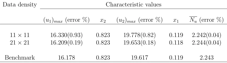
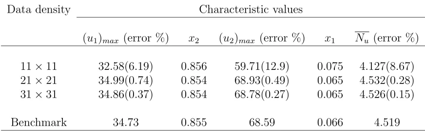
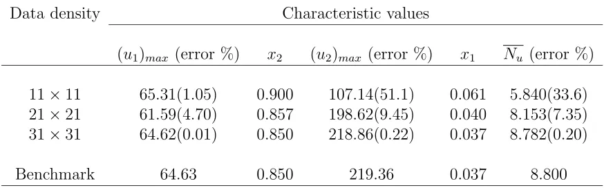
Integrals (44) and (43) are computed using Simpson rule. Results of (u₁)_max, (u₂)_max, their positions and N_u for Ra = {104,105,106,107} are displayed in Ta-bles 3-6, respectively, where finer densities are used for higher Ra values. In all

cases, the errors relative to the benchmark solutions consistently reduce with an

increase in data density, indicating “mesh convergence”.

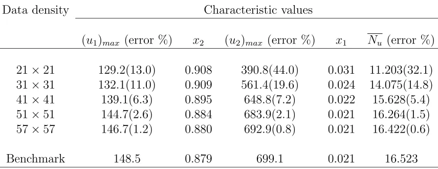
The successful simulations of natural convection flow at Ra = 107 using relatively coarse densities (21×21,· · · ,57×57) demonstrate the effectiveness of the proposed

methods. As can be seen from Figure 4, velocity boundary layers significantly

increase in strength with an increasing Rayleigh number.

General results for flow at Ra = 107 in the form of stream function, vorticity and temperature contour plots are displayed in Figure 5. Each plot draws 21 contour

lines whose values vary uniformly from the minimum to maximum values. The

temperature, vorticity and stream function fields are skew-symmetric with regard

to the geometric centre of the cavity (centro-symmetric).

6

CONCLUDING REMARKS

Two versions of indirect RBFNs are developed for the numerical solution of

high-order PDEs. In the first version, the IRBFN formulations are written directly in

terms of network weights, while in the second version, they are expressed in terms

of nodal variable values. The first version is more straightforward to implement, but

produces much larger system matrices than the second version. The emphasis here

is placed on the advantages of using integration in constructing neural networks with

regard to the implementation of multiple boundary conditions (straightforwardly)

and the approximation of high-order derivatives (accurately). The present

thin-plate bending problems and natural convection flows which are governed by

biharmonic equations. Accurate results and high rates of convergence are achieved.

APPENDIX

The following are new basis functions obtained from integrating MQ-RBFs by using

MATHEMATICA.

H_[[3](_x i)

j] =

(x_j−c(_ji))

2 A+

C

2B, (45)

H_[[2](_x i)

j] =

(x_j −c(_ji))2

6 −

C

3

A+ C(xj−c

(i)

j )

2 B, (46)

H_[[1](_x i)

j] =

(x_j −c(_ji))3

24 −

13C(x_j−c(_ji)) 48

A+

C(x_j−c(_ji))2

4 −

C2

16

B, (47)

H_[[0](_x i)

j] =

C2

45 −

83C(x_j−c(_ji))2

720 +

(x_j−c(_ji))4 120

A+

4C(x_j −c(_ji))3

48 −

3C2(x_j −c(_ji)) 48

B, (48)

where

r=x−c(i), A=r2+a(i)2, B = ln

(x_j −c(_ji)) +r2+a(i)2

, C =r2−(x_j−c_j(i))2+a(i)2.

ACKNOWLEDGEMENTS

N. Mai-Duy wishes to thank the University of Sydney for a Sesqui postdoctoral

research fellowship. The computing facilities provided by the APAC National

Fa-cilities are greatly acknowledged. The authors would like to thank the referees for

their helpful comments.

1. Haykin S. Neural Networks: A Comprehensive Foundation. Prentice-Hall:

New Jersey, 1999.

2. Kansa EJ. Multiquadrics- A scattered data approximation scheme with

appli-cations to computational fluid-dynamics-II. Solutions to parabolic, hyperbolic

and elliptic partial differential equations. Computers and Mathematics with

Applications 1990; 19(8/9): 147-161.

3. Mai-Duy N, Tran-Cong T. Numerical solution of differential equations using

multiquadric radial basis function networks. Neural Networks 2001; 14(2):

185-199.

4. Sharan M, Kansa EJ, Gupta S. Application of the multiquadric method for

numerical solution of elliptic partial differential equations. Journal of Applied

Science and Computation 1997; 84: 275-302.

5. Zerroukat M, Power H, Chen CS. A numerical method for heat transfer

prob-lems using collocation and radial basis functions. International Journal for

Numerical Methods in Engineering 1998; 42: 1263-1278.

6. Mai-Duy N, Tran-Cong T. Numerical solution of Navier-Stokes equations

us-ing multiquadric radial basis function networks. International Journal for

Numerical Methods in Fluids 2001; 37: 65-86.

7. Larsson E, Fornberg B. A numerical study of some radial basis function based

solution methods for elliptic PDEs. Computers and Mathematics with

Appli-cations 2003; 46: 891-902.

8. Shu C, Ding H, Yeo KS. Local radial basis function-based differential

quadra-ture method and its application to solve two-dimensional incompressible

Navier-Stokes equations. Computer Methods in Applied Mechanics and Engineering

9. Sarler B, Perko J, Chen CS. Radial basis function collocation method solution

of natural convection in porous media. International Journal of Numerical

Methods for Heat & Fluid Flow 2004; 14(2): 187-212.

10. Mai-Duy N. Solving high order ordinary differential equations with radial basis

function networks. International Journal for Numerical Methods in

Engineer-ing 2005;62: 824-852.

11. Canuto C, Hussaini MY, Quarteroni A, Zang TA. Spectral Methods in Fluid

Dynamics. Springer-Verlag: New York, 1988.

12. Jang SK, Bert CW, Striz AG. Application of differential quadrature to static

analysis of structural components. International Journal for Numerical

Meth-ods in Engineering 1989; 28(3): 561-577.

13. Wang X, Bert CW. A new approach in applying differential quadrature to

static and free vibrational analyses of beams and plates. Journal of Sound

and Vibration 1993; 162(3): 566-572.

14. Shu C, Du H. Implementation of clamped and simply supported boundary

con-ditions in the GDQ free vibration analysis of beams and plates. International

Journal of Solids and Structures 1997; 34(7): 819-835.

15. Shu C, Du H. A generalized approach for implementing general boundary

conditions in the GDQ free vibration analysis of plates. International Journal

of Solids and Structures 1997; 34(7): 837-846.

16. Liu GR, Wu TY. Multipoint boundary value problems by differential

quadra-ture method. Mathematical and Computer Modelling 2002; 35: 215-227.

17. Shu C. Differential Quadrature and Its Application in Engineering.

18. Press WH, Flannery BP, Teukolsky SA, Vetterling WT. Numerical Recipes in

C: The Art of Scientific Computing. Cambridge University Press: Cambridge,

1988.

19. Park J, Sandberg IW. Universal approximation using radial basis function

networks. Neural Computation 1991; 3: 246-257.

20. Franke R. Scattered data interpolation: tests of some methods. Mathematics

of Computation 1982; 38(157): 181-200.

21. Madych WR, Nelson SA. Multivariate interpolation and conditionally positive

definite functions. Approximation Theory and its Applications1989; 4: 77-89.

22. Madych WR, Nelson SA. Multivariate interpolation and conditionally positive

definite functions, II. Mathematics of Computation 1990; 54(189): 211-230.

23. Zeb A, Elliott L, Ingham DB, Lesnic D. A comparison of different methods to

solve inverse biharmonic boundary value problems. International Journal for

Numerical Methods in Engineering 1999; 45: 1791-1806.

24. Timoshenko S, Woinowsky-Krieger S. Theory of Plates and Shells.

McGraw-Hill: New York, 1959.

25. Leissa AW. The free vibration of rectangular plates. Journal of Sound and

Vibration 1973; 31: 257-293.

26. Leonard BP, Drummond JE. Why you should not use ‘Hybrid’, ‘Power law’

or related exponential schemes for convective modelling-there are much better

alternatives. International Journal for Numerical Methods in Fluids1995;20:

421-442.

27. Roache PJ. Verification and Validation in Computational Science and

28. de Vahl Davis G. Natural convection of air in a square cavity: a bench mark

numerical solution. International Journal for Numerical Methods in Fluids

1983; 3: 249-264.

29. Le Quere P. Accurate solutions to the square thermally driven cavity at high

Rayleigh number. Computers & Fluids1991; 20(1): 29-41.

30. McCartin BJ. A model-trust region algorithm utilizing a quadratic interpolant.

Table 1: Clamped rectangular plates of dimension [−a/2, a/2]×[−b/2, b/2] under a uniform loadq, 11×11 data points: deflections at the centre and bending moments at (x₁ = a/2, x₂ = 0). The computed solutions are in good agreement with the analytical solutions [24].

v/(qa4/D)×102 M_x/(qa2)×10

b/a IRBFN analytical IRBFN analytical

1.0 0.1265 0.126 -0.5138 -0.513

1.1 0.1507 0.150 -0.5813 -0.581

1.2 0.1724 0.172 -0.6392 -0.639

1.3 0.1911 0.191 -0.6871 -0.687

1.4 0.2068 0.207 -0.7259 -0.726

1.5 0.2196 0.220 -0.7565 -0.757

1.6 0.2300 0.230 -0.7802 -0.780

1.7 0.2382 0.238 -0.7982 -0.799

1.8 0.2446 0.245 -0.8116 -0.812

1.9 0.2495 0.249 -0.8214 -0.822

Table 2: Free vibration, simply supported plate, [0,1]×[0,1]: natural frequencies. The present results agree well with those obtained by the DQ method [17] and the Rayleigh-Ritz (R-R) method [25]. By regarding the results from the R-R method as exact solutions, it can be seen that the errors (%) consistently reduce with an increase in data density.

IRBFN DQ R-R

Ω 7×7(error) 9×9(error) 11×11(error) 12×12(error)

Table 3: Natural convection flow, Ra= 104.

Data density Characteristic values

(u₁)_max (error %) x₂ (u₂)_max (error %) x₁ N_u (error %)

11×11 16.330(0.93) 0.823 19.778(0.82) 0.119 2.242(0.04)

21×21 16.209(0.19) 0.823 19.653(0.18) 0.118 2.244(0.04)

Table 4: Natural convection flow, Ra= 105.

Data density Characteristic values

(u₁)_max (error %) x₂ (u₂)_max (error %) x₁ N_u (error %)

11×11 32.58(6.19) 0.856 59.71(12.9) 0.075 4.127(8.67)

21×21 34.99(0.74) 0.854 68.93(0.49) 0.065 4.532(0.28)

31×31 34.86(0.37) 0.854 68.78(0.27) 0.065 4.526(0.15)

Table 5: Natural convection flow, Ra= 106.

Data density Characteristic values

(u₁)_max (error %) x₂ (u₂)_max (error %) x₁ N_u (error %)

11×11 65.31(1.05) 0.900 107.14(51.1) 0.061 5.840(33.6)

21×21 61.59(4.70) 0.857 198.62(9.45) 0.040 8.153(7.35)

31×31 64.62(0.01) 0.850 218.86(0.22) 0.037 8.782(0.20)

Table 6: Natural convection flow, Ra= 107.

Data density Characteristic values

(u₁)_max (error %) x₂ (u₂)_max (error %) x₁ N_u (error %)

21×21 129.2(13.0) 0.908 390.8(44.0) 0.031 11.203(32.1)

31×31 132.1(11.0) 0.909 561.4(19.6) 0.024 14.075(14.8)

41×41 139.1(6.3) 0.895 648.8(7.2) 0.022 15.628(5.4)

51×51 144.7(2.6) 0.884 683.9(2.1) 0.021 16.264(1.5)

57×57 146.7(1.2) 0.880 692.9(0.8) 0.021 16.422(0.6)

v, ∂v/∂x₂ (v, ∂2v/∂x2₂)

v, ∂v/∂x₂ (v, ∂2v/∂x2₂)

v

,

∂v

/

∂

x1

(

v

,

∂

2 v/

∂

x

2 1)

v

,

∂v

/

∂

x1

(

v

,

∂

2 v/

∂

x

2 1)

x₁ x₂

o

10−0.6 10−0.5 10−0.4 10−0.3 10−0.2 10−0.1 100 100.1

10−7

10−6

10−5

10−4

10−3

10−2

10−1

100

v u

Centre spacing Ne

Figure 2: Biharmonic problem, domain [−2,2]×[−2,2], boundary conditionsv and

10−0.6 10−0.5 10−0.4 10−0.3 10−0.2 10−0.1 100 100.1

10−5

10−4

10−3

10−2

10−1

100

v u

Centre spacing Ne

Figure 3: Biharmonic problem, domain [−2,2]×[−2,2], boundary conditionsv and

−1500 −100 −50 0 50 100 150 0.1

0.2 0.3 0.4 0.5 0.6 0.7 0.8 0.9 1

Ra=107 Ra=106 Ra=105

u₁

x2

0 0.1 0.2 0.3 0.4 0.5 0.6 0.7 0.8 0.9 1 −800

−600 −400 −200 0 200 400 600 800

Ra=107 Ra=106 Ra=105

x₁

u2

a) stream function

b) vorticity

c) temperature