Fast-response piezoresistive pressure transducers for thermofluids experiments

(1)

Faculty of Engineering & Surveying

Fast-Response Piezoresistive Pressure Transducers For

Thermofluids Experiments

A dissertation submitted by

Peter Hockings

in fulfilment of the requirements of

ENG4112 Research Project

towards the degree of

Bachelor of (Mechanical Engineering)

(2)

Abstract

Thermofluids experiments often require the use of fast-response pressure transducers that maintain their accuracy over a wide range of operating temperatures. Existing pressure sensing technologies are available which suit these demanding applications, however these transducers are usually relatively expensive. This project investigates the use of inexpensive piezoresistive pressure transducers in the measurement of transient fluid pressures.

A temperature compensation routine was developed which improved the accuracy of the piezoresistive pressure transducers over a substantial range of operating tempera-tures. A dynamic response analysis indicated that the diaphragm resonant frequency of these sensors was 246.7 kHz (without the addition of latex or grease) and that the response times could be improved from approximately 12.5 µsto 0.38 µs with simple case modifications. These results demonstrated the suitability of piezoresistive pressure transducers for use in fast-response thermofluids experiments.

(3)

Faculty of Engineering and Surveying

ENG4111/2 Research Project

Limitations of Use

The Council of the University of Southern Queensland, its Faculty of Engineering and Surveying, and the staff of the University of Southern Queensland, do not accept any responsibility for the truth, accuracy or completeness of material contained within or associated with this dissertation.

Persons using all or any part of this material do so at their own risk, and not at the risk of the Council of the University of Southern Queensland, its Faculty of Engineering and Surveying or the staff of the University of Southern Queensland.

This dissertation reports an educational exercise and has no purpose or validity beyond this exercise. The sole purpose of the course pair entitled “Research Project” is to contribute to the overall education within the student’s chosen degree program. This document, the associated hardware, software, drawings, and other material set out in the associated appendices should not be used for any other purpose: if they are so used, it is entirely at the risk of the user.

Prof G Baker

Dean

(4)

Certification of Dissertation

I certify that the ideas, designs and experimental work, results, analyses and conclusions set out in this dissertation are entirely my own effort, except where otherwise indicated and acknowledged.

I further certify that the work is original and has not been previously submitted for assessment in any other course or institution, except where specifically stated.

Peter Hockings

Q11219289

Signature

(5)

Acknowledgments

I would like to sincerely thank the following individuals for their assistance in my work. Without the support of these people this project could not have reached completion.

Dr. David Buttsworth for his guidance and patience. Even with such a large number of project students, David was still able to find the time to lend assistance when it was needed.

Dr. Ahmad Sharifian for his assistance in the last few weeks of semester 2, once David had left for England.

The staff from the mechanical and electrical workshops for their vital contributions of supplying and manufacturing various components.

Finally, a special thankyou to my family, college friends and my girlfriend Emily. The understanding and support of these people was invaluable to the successful completion of this dissertation.

Peter Hockings

University of Southern Queensland

(6)

List of Figures

2.1 The Sensym 13U Stainless Steel Pressure Transducer (Honeywell/Sensym) 5

2.2 Basic Structure of Piezoresistive Pressure Transducer (MAXIM 2001) . 6

2.3 Wheatstone Circuit of the Pressure Transducer (Honeywell) . . . 7

2.4 The comparison of outputs between an uncompensated pressure sensor (a) and a sensor compensated for temperature changes (b) (Ainsworth et al. 2000) . . . 8

2.5 Basic circuit to determine Vsense (Ainsworth et al. 2000) . . . 9

2.6 Output of a piezoresistive pressure transducer after a step input pressure signal (Ainsworth et al. 2000) . . . 10

2.7 The power spectrum from a typical step response, showing the resonant frequency at the dominant peak on the graph (Ainsworth et al. 2000) . 11

3.1 The ‘Dead Weight’ tester used for the static calibrations . . . 17

3.2 Conditioning Circuit to determine Vsense . . . 18

3.3 Oven used for temperature calibrations . . . 19

(13)

3.5 The USQ Gun Tunnel used for experimental testing . . . 21

4.1 A block diagram, showing the approached used for the static calibrations 27 4.2 A photograph of the electrical circuit used to produce the sensor outputs, Vout and Vsense . . . 28

4.3 Static calibration of Sensym SX150AHO sensor . . . 29

4.4 Static calibration of Sensym 13U3000 sensor . . . 30

4.5 Static calibration of Sensym 13U0500 sensor . . . 31

4.6 The modified oven (right) and the Dead Weight tester (left) used for temperature calibrations . . . 33

4.7 The Positive Linear Relationship between Vsense and Sensor Temperature 35 4.8 The Positive Linear Relationship between Span and Sensor Temperature 36 4.9 The Relationship between Offset and Sensor Temperature . . . 37

4.10 Error from an uncompensated piezoelectric sensor . . . 40

4.11 Error from a compensated piezoelectric sensor . . . 41

5.1 Photograph of the shock tube used to test the sensor dynamic charac-teristics . . . 44

5.2 Schematic diagram of Shock Tube showing positions of pressure sensors 45 5.3 A block diagram, showing the method of pressure measurement for shock tube tests . . . 45

(14)

5.5 A typical sensor response and a comparison between measured and pre-dicted reflected shock pressures. . . 50

5.6 A typical long time scale sensor response and a comparison between measured and predicted reflected shock pressures. . . 51

5.7 Comparison of sensor response and theoretical internal pressure over time for shock test 2 . . . 53

5.8 Comparison of sensor response and a possible theoretical model of in-ternal pressure over time for shock test 2, given that the shock wave increases the internal pressure of the sensor to 250kPa . . . 54

5.9 Sensor output from Shock Tube test 4, demonstrating multiple modes of vibration . . . 55

5.10 The power spectrum density of Shock Tube test 4, showing the resonant frequency of the silicon diaphragm . . . 57

5.11 The amplitude ratio and phase shift for relative frequency ratios (Ainsworth et al. 2000) . . . 60

5.12 The 10 and 90% lines used to measure the response time of the sensor . 62

6.1 A schematic diagram of the USQ Gun Tunnel in the format used for this project (Top View) . . . 67

6.2 Mountings of piezoresistive and piezoelectric sensors in the Gun Tunnel barrel (note: the end of the barrel is unsealed at this stage) . . . 68

6.3 A block diagram, showing the method of pressure measurement for the USQ Gun Tunnel . . . 69

(15)

6.5 A comparison between the piezoresistive and piezoelectric pressure sen-sors after the peak Gun Tunnel pressure . . . 71

6.6 A comparison between the smoothed piezoresistive data and the piezo-electric sensor output . . . 72

6.7 A comparison between the smoothed piezoresistive and piezoelectric pressure sensors after the peak Gun Tunnel pressure . . . 72

7.1 A photograph showing the mounting of the piezoelectric (right) and piezoresistive (left) sensors on the engine . . . 75

7.2 The Shaft Encoder attached to the engine . . . 76

7.3 A block diagram, showing the method of pressure measurement for the internal combustion engine . . . 77

7.4 The layout of the engine testing apparatus . . . 77

7.5 Engine pressures determined from the piezoresistive and piezoelectric pressure transducers - motored, closed throttle . . . 78

7.6 Engine pressures determined from the piezoresistive and piezoelectric pressure transducers - fired, closed throttle, no load . . . 79

7.7 Engine pressures determined from the piezoresistive and piezoelectric pressure transducers - fired, closed throttle, loaded . . . 79

7.8 Engine pressures determined from the piezoresistive and piezoelectric pressure transducers - fired, open throttle, loaded . . . 80

7.9 A comparison between the theoretical and measured cylinder pressures - motored . . . 82

(16)

List of Tables

3.1 Engine Specifications for the Kubota GS200 Petrol Engine . . . 23

4.1 Sensor Characteristics for Sensym 13U0500 Piezoresistive Pressure Trans-ducer - Experimental Values and Manufacturer’s Specifications (Exper-imental Offset coefficient for 27 to 97◦_{C, Manufacturer’s Spec. Offset}

coefficient for 0 to 82◦_{C) . . . .} ₃₇

5.1 Summary of sensor modifications used for shock tube tests . . . 47

5.2 Shock Tube tests and corresponding sensors used . . . 48

5.3 Comparison between theoretical and measures reflected shock pressures) 52

5.4 Diaphragm resonant frequencies determined from power spectrum den-sity analysis (a resonant frequency of 0Hz indicates that no clear fre-quency was identified) . . . 58

5.5 Response times for sensor outputs for each of the Shock Tube tests . . . 63

(17)

Introduction

This project investigates the performance characteristics of piezoresistive pressure trans-ducers under high temperature operation and transient pressure measurement. Static calibrations and temperature compensation will be investigated as well as the dynamic response characteristics of the piezoresistive pressure transducers. These sensors will be applied to measurement of the cylinder pressures of an internal combustion engine and pressures within the USQ Gun Tunnel. The measurements taken with these pres-sure sensors can then be analysed and compared with similar data produced from other available types of transducers and various theoretical methods. The performance and suitability of piezoresistive pressure sensors for these applications can then be evaluated.

1.0.1 Project Aims and Objectives

This project aims to identify the frequency and temperature response characteristics of low cost piezoresistive pressure transducers and provide accurate calibration to allow these pressure sensors to be used with a high degree of confidence in fast-response thermofluids experiments.

The specific objectives of the project are as follows

(18)

piezoresistive pressure measurement devices.

2. Devise appropriate electrical circuits to implement such techniques.

3. Devise suitable apparatus for quasi-static calibration of pressure transducers for both pressure and temperature sensitivity.

4. Perform calibrations on selected transducers.

5. Investigate the dynamic response of sensors of various configurations (added grease, modified cases etc.) using a shock tube calibration.

6. Obtain pressure measurements in a Gun Tunnel.

7. Analyse the measurements from the Gun Tunnel and compare with data obtained from a piezoelectric sensor.

8. Obtain pressure measurements in an IC engine.

9. Analyse the measurements from the IC engine and compare with data obtained from a piezoelectric sensor.

as time permits

-10. Compare the measurements from the Gun Tunnel with predictions based on a computational model (Lagrangian quasi one dimensional).

11. Compare the measurements from the IC engine with predictions based on a com-putational model (thermodynamic engine simulation).

1.1

Overview of the Dissertation

This dissertation is organized as follows:

Chapter 2 covers the literature review, background and assessment of consequential effects.

(19)

Chapter 4 discusses static sensor calibration and temperature compensation tech-niques for piezoresistive sensors.

Chapter 5 covers the testing and analysis of the dynamic response characteristics of the piezoresistive sensors.

Chapter 6 investigates the application of measuring pressures within the Gun Tunnel using piezoresistive pressure sensors.

Chapter 7 examines the use of piezoresistive pressure transducers in the measurement of cylinder pressures of an IC engine

(20)

Background, Literature Review

and Assessment of Consequential

Effects

2.1

Project Background

Experimental testing facilities (including Gun Tunnels and Shock Tubes) and common machinery (such as the internal combustion engine) may require the measurement of internal pressures (both static and dynamic). This allows an analysis of their perfor-mance and provides further understanding of the thermofluids process that occur.

(21)

Typically, piezoresistive pressure transducers have been used for the measurement of static or quasi-static pressure levels. This project aims to test the dynamic response characteristics of the sensors and investigate the feasibility of using these piezoresistive sensors for fast response measurements. The temperature effects on the sensors will also be analysed. This will ultimately allow a temperature compensation technique that maintains accurate pressure measurements in a wide variety of harsh operational environments.

2.2

Literature Review

2.2.1 Background - Piezoresistive Pressure Transducers

The typical fast-response piezoresistive pressure transducer relies on accurately mea-suring the deflection of a diaphragm (typically silicon) that is caused by fluid pressures. These sensors are generally low cost and can be implemented in a wide variety of ap-plications. A diagram of a typical piezoresistive pressure transducer is shown in figure 2.1.

Figure 2.1: The Sensym 13U Stainless Steel Pressure Transducer (Honeywell/Sensym)

Some advantages associated with the piezoresistive pressure transducer are (Microsys-tems),

• Low-cost sensor fabrication opportunity.

(22)

• Different pressure levels can be achieved according to the application.

• Wide range of pressure sensitivities.

• Read-out circuitry can be either on-chip or discrete.

There are also some disadvantages of piezoresistive pressure sensors (MAXIM 2001),

• Strong nonlinear dependence of the full-scale signal on temperature (up to 1%/kelvin)

• Large initial offset (up to 100% of full scale or more)

• Strong drift of offset with temperature

The disadvantages associated with temperature dependance can be overcome (or at least, greatly reduced) using the temperature compensation techniques discussed in later sections.

The basic construction of the piezoresistive pressure transducer is shown in figure 2.2.

Figure 2.2: Basic Structure of Piezoresistive Pressure Transducer (MAXIM 2001)

Using diffusion methods, 4 piezoresistive elements are positioned on the top surface of the diaphragm. The elements change their resistance according to the level of strain. Therefore, as the diaphragm deflects (due to the fluid pressure), the resistance of each of the elements change.

(23)

under compression and two to be placed under tension as the diaphragm deflects. This causes the resistance to increase in two elements, and decrease in the remaining two. This change in resistance is represented by ∆R in figure 2.3. The shift in the values of resistance causes a voltage difference between V1 and V2. This voltage difference is measured as the value of Vout. The value of Vout is linearly related to the applied fluid

[image:23.595.240.397.236.357.2]

pressure.

Figure 2.3: Wheatstone Circuit of the Pressure Transducer (Honeywell)

The transducer sensitivity can be determined through a static calibration process. The value of Voutmay then be used to calculated the fluid pressure applied to the transducer.

Advances in production technology, such as the rapid developments in the semiconduc-tor industry in the 1960s (Ainsworth et al. 2000), have enabled piezoresistive pressure transducers to become more compact, improved the quality of construction and mini-mizing the cost of production.

2.2.2 Temperature Compensation

One major issue in the use of piezoresistive pressure transducers is their temperature sensitivity. The output of the sensor may therefore require compensation for tempera-ture effects. Temperatempera-ture related errors may severely compromise the sensor accuracy under operation in extreme hot or cold environments.

(24)

[image:24.595.183.456.101.491.2]

Figure 2.4: The comparison of outputs between an uncompensated pressure sensor (a) and a sensor compensated for temperature changes (b) (Ainsworth et al. 2000)

The output from a piezoresistive pressure transducer relies on two basic characteristics, the sensor Span (or sensitivity) and the sensor Offset (the sensor output at zero abso-lute pressure) (Ainsworth, Miller, Moss & Thorpe 2000, Denos 2002, Clark 1992). The values for Span and Offset change with temperature therefore errors are introduced when taking pressure measurements from relatively hot or cold environments. Com-pensation methods have been developed to take the temperature sensitivity of Span and Offset into account. These techniques allow a more consistent accuracy from the pressure transducers.

(25)

and Denos (2002) assumed a linear relationship between sensor Offset and Span with temperature, however these investigations incorporated a much smaller temperature range. Each of these temperature compensation methods allows a post-experimental routine, where the recorded sensor output voltage and temperature can be used to accurately determine fluid pressure.

Figure 2.5: Basic circuit to determine Vsense (Ainsworth et al. 2000)

To indicate the temperature of the sensor (and allow the temperature correction to be applied), the conditioning circuit shown in figure 2.5 was implemented by both Ainsworth et al. (2000) and Denos (2002). This circuit incorporates the pressure trans-ducer into a Wheatstone bridge. The overall resistance of the pressure transtrans-ducer will vary with temperature, and the temperature of the other resistors in the external circuit will remain constant (causing the resistance of the external circuit to remain constant). A change in the sensor temperature will therefore result in a change in the voltage, Vsense. The value of Vsense is then used to calculate the temperature of the sensor.

A temperature compensation routine can ultimately be applied to the pressure sensor output (demonstrated by Ainsworth et al. (2000) and Denos (2002)).

(26)

Temperature calibrations conducted by Ainsworth et al. (1991) assumed that with short experimental run times, only minor temperature changes would be expected. For experimental situations with a significant and sustained operational temperature (eg. testing in-cylinder engine pressures), the static temperature compensation methods mentioned previously can be applied.

2.2.3 Dynamic Response Calibration

The dynamic response characteristics of the piezoresistive pressure transducer deter-mine it suitability for use in fast-response thermofluids experiments.

[image:26.595.183.460.459.668.2]

Shock tubes can be used in experimental testing for the analysis of the dynamic re-sponse of the pressure transducers (eg. Ainsworth et al. 1991). The results from these tests reveal that certain frequencies become dominant in the response of the pressure sensor (these are the resonant frequencies of the pressure transducer). A typical sensor response to a step input can be observed in figure 2.6 and the related power spectrum demonstrating the resonant frequency is given in figure 2.7.

Figure 2.6: Output of a piezoresistive pressure transducer after a step input pressure signal (Ainsworth et al. 2000)

(27)

[image:27.595.180.461.103.323.2]

Figure 2.7: The power spectrum from a typical step response, showing the resonant frequency at the dominant peak on the graph (Ainsworth et al. 2000)

creates sounds waves of variable frequency. These sound waves then cause pressure variations at the pressure transducer. This allows the amplitude response and phase shift of the transducer to be analysed over a wide range of operational frequencies. As stated by Boerrigter & Charbonnier (1997), this has advantages over a shock tube tests since this technique easily identifies the resonant frequencies of other bodies (such as the air adjacent of the transducer) and the pressure and temperature of the test are known (the precise shock conditions in a shock tube test are difficult to determine).

Analytical techniques for the calculation of dynamic response were also demonstrated by Ainsworth et al. (2000) and Boerrigter & Charbonnier (1997). Ainsworth et al. (2000) have taken the approach of approximating the piezoresistive pressure transducer with a transfer function, which provides data about the expected frequency response of the system. This approach gives theoretical simulations for the transducer phase shift and amplitude. Boerrigter & Charbonnier (1997) developed an analytical model from key dynamics and fluid mechanics formulas that can also ultimately be used to predict the frequency response of a pressure measurement system.

(28)

of the transducer itself. Articles from Boerrigter & Charbonnier (1997) investigate the use of analytical calculations to determine the resonant frequency of the air in front of the diaphragm. Once the resonant frequencies of the piezoresistive pressure transducer have been measured, it can be determined whether these frequencies are related to the resonance of the air around the sensor or the resonance of the silicon diaphragm.

A layer of grease or a flexible compound may be used to cover the diaphragm on the pressure sensor. This procedure is designed to protect the pressure sensor from particles that may impact on the diaphragm and damage the sensor (Ainsworth et al. 2000, Buttsworth & Jacobs 2000). Experiments involving sensors with and without silastomer demonstrated that the silastomer layer significantly increased the damping ratio of the sensor response (Ainsworth et al. 2000).

2.3

Assessment of Consequential Effects

While this project focuses largely on short term results and immediate outcomes, long term effects of this research must also be considered. These effects include the aspects of sustainability, ethical responsibility and safety issues.

2.3.1 Substantiality

Environmental sustainability is of continually increasing importance to modern engi-neering practices. The short, medium and long term environmental consequences of an engineering task (such as the work undertaken on this project) must be anticipated. Where negative effects are apparent, actions need to be taken to minimize or remove any environmental damage.

While this project has a minimal environmental impact in terms of direct pollution created or environmental degradation caused, there are other non-direct environmental impacts associated with this research topic, including

(29)

• The resource requirements for experimental testing

The components used in this project (the pressure sensors and the developed testing apparatus) make use of finite resources for their production (metals and plastics). For-tunately these products are mostly recyclable. The pressure sensors themselves can be reused for different pressure measurement applications and offer a reasonable service life (depending on the severity of the testing environment). The other materials used for the construction of the testing apparatus are readily recyclable (plastics, metals and electrical components) therefore the waste from this project can be minimized.

Some of the experimental testing procedures may require non-renewable resources. This project will require the use of internal combustion engines (for use in pressure testing and for powering other experiments) which use fossil fuels and produce harmful emissions. While these are negative environmental effects, these experiments will only be conducted over a short period during the experimental stages of the project.

The results from this project may ultimately contribute to environmental sustainability. If these pressure sensors are widely available at low cost, machinery and manufactur-ing process could be more readily monitored and their efficiency could be maximized. This could lead to a reduction of pollutants created and contribute towards a cleaner environment.

2.3.2 Ethical Responsibility

Most new technologies have associated ethical implications related to the particular outcomes of that development. Therefore an ethical responsibility exists where the engineer must consider the people who are affected.

This project makes heavy use of relatively new technologies and the possible outcomes of this research may also bring further advancement to the area of piezoresistive pressure sensor technology. The range of possible ethical consequences were considered before commitment to this project.

(30)

tech-nology becomes widely implemented. Ultimately this project may allow a reduction in the use of highly expensive pressure transducers. This may adversely affect some suppliers and sensor producers. Fortunately the suppliers and manufacturers typically use a wide range of products, therefore if a small number of items became obsolete due to the piezoresistive technology, the consequences would be minimal.

(31)

2.4

Chapter Summary

This chapter has investigated background knowledge and previous research related to the field of piezoresistive pressure transducers. Past experiments and models used to test the dynamic characteristics and temperature compensations for piezoresistive sen-sors provide possible techniques that could be used for this project or similar research.

(32)

Design Methodology

3.1

Static Calibrations and Temperature Compensation

for Pressure Sensors

The pressure and temperature sensitivity of piezoresistive pressure transducers can be determined through a series of static calibrations. These calibrations allow accurate results to be obtained from experimental testing.

The static calibration process will initially begin by testing the pressure sensitivity of the pressure transducers at room temperature (approximately 25◦_{C). These static}

tests will be conducted using the ‘Dead Weight’ tester (shown in figure 3.1). The Dead Weight testers allows precise levels of pressure to be applied to the pressure sensor.

(33)

Sensors 17

Figure 3.1: The ‘Dead Weight’ tester used for the static calibrations

calibration experimentation.

The output voltage of the pressure transducer(Vout) relates directly to the applied

pressure. This typically results in a highly linear relationship between these two vari-ables. The output of the transducer can be correlated to pressure using the equation 4.1 (Ainsworth et al. 2000, Denos 2002),

V =SP +O (3.1)

In equation 4.1, ‘V’ is the output voltage (or Vout), ‘S’ is the senor span (or sensitivity)

and ‘O’ is the sensor offset (the voltage output, Vout, at zero absolute pressure). This

function can be used to accurately determine the pressure from the sensor output voltage while the pressure transducer is at room temperature.

As the temperature of the sensor changes, the values for Span and Offset also change. It is critical to determine the how these characteristics change with temperature. High temperature thermofluids experiments (such as testing the in-cylinder pressures on the IC engine) will produce inaccurate results if no temperature corrections are applied.

(34)

Sensors 18

a circuit as shown in figure 3.2. This electrical circuit is adapted from the work of Ainsworth et al. (2000).

Figure 3.2: Conditioning Circuit to determine Vsense

(Ainsworth et al. 2000)

As the overall resistance of the pressure transducer changes with temperature, the value for Vsense will also shift.

A range of different pressures can be applied to the pressure transducer while it is held at selected constant temperatures (approximately ranging from room temperature to 150◦_{C). This will be achieved by placing the pressure transducer in the oven shown in}

figure 3.3, and attaching a remote connection to the Dead Weight tester (figure 3.1).

The relationship between sensor output voltage, and applied pressure, allow values for Span and Offset to be calculated at a range of different testing temperatures. The rate of change of sensor Span and Offset with temperature can then be determined.

One particular method, developed by Ainsworth et al. (2000), applied the temperature correction directly to the value of Vout. A function was developed that uses the values

(35)

Sensors 19

Figure 3.3: Oven used for temperature calibrations

sensor. The temperature of the sensor is determined by the corresponding value for Vsense. This corrected value for Vout, known as V*out, is the predicted output that

the sensor would produce if it were at room temperature. This function is shown in equation 3.2.

V∗ ₌_V

µ

1− 1

S25

dS

dT∆T

¶

−O25

µ

1− 1

S25

dS

dT∆T

¶

−dO

dT∆T

µ

1− 1

S25

dS

dT∆T

¶

(3.2)

The value of V* (or V*out) can then be used with the room temperature values of

span (S25) and offset (O25) to allow the true experimental pressure to be determined (equation 3.3).

V∗ ₌_S

(36)

3.2

Testing of Dynamic Response Characteristics

The dynamic response characteristics of the piezoresistive pressure transducers deter-mines the behavior of the pressure sensors under high frequency changes in fluid pres-sures. Dynamic response testing allows the maximum operational frequencies of the pressure transducers to be deduced. As experimental pressure fluctuation frequencies reach the maximum operational frequency of the pressure transducer, errors begin to occur in the output of the sensor.

The dynamic response properties of the piezoresistive pressure transducers will be tested using a shock tube (as shown in figure 3.4).

Figure 3.4: Basic Shock Tube design, similar to the apparatus used for this project

(Boerrigter & Charbonnier 1997)

A shock wave is produced within the tube when a diaphragm is ruptured. This wave of pressure travels at high speed along the tube and reflects off the end face. The pressure transducer, mounted level with the end face of the tube, undergos an approximate step input (since the change in pressure is very rapid). The response of the transducer to this input then allows the dynamic response characteristics to be determined. These characteristics include values such as response time and resonant frequency.

(37)

The test results from the shock tube can also be used to find the response time of the pressure transducers. This will determine the suitability and general accuracy of the pressure sensors under fast response testing applications. In these transient pressure measurement applications short response times are essential for recording an accurate set of readings.

Shock tube tests can also be conducted to test the dynamic response characteristics of modified pressure sensors. Various configurations of sensors, including sensors with modified cases and added grease or silastomer, will be tested to investigate the effects of these changes on the sensor response. These modifications are expected to provide pro-tection to the silicon diaphragm of the sensor (with the addition of grease or silastomer) and possibly improve the response time of the sensors (with case modifications).

3.3

Pressure Testing with the USQ Gun Tunnel

[image:37.595.160.482.499.743.2]

The static calibration operations and dynamic response analysis lead to testing in facil-ities such as the USQ Gun Tunnel. This apparatus (shown in figure 3.5) (Buttsworth n.d.) is capable of producing a high speed, short duration gas flow.

(38)

The short period of the actual test flow (typically milliseconds) demands that the pres-sure sensors used to analyse the test gas has a very short response time. It is assumed that thermal effects from the hot gases on the sensor are negligible, since the short test times will not allow the pressure transducer to significantly change temperature while results are being recorded.

The results obtained from the Gun Tunnel with the piezoresistive pressure sensor are then able to be compared to the output from a piezoelectric pressure transducer (an expensive sensor, well suited to this measurement application). This gives an indication of the accuracy of the static calibration of the piezoresistive sensors and also shows a comparison between the dynamic characteristics of the two sensors.

If time permits, a theoretical analysis of the Gun Tunnel may also be conducted, using computational methods. This allows a comparison between theoretical pressures and the results from the output from the piezoresistive pressure transducer.

3.4

Pressure Testing with an IC Engine and Theoretical

Analysis

Pressure measurement within an internal combustion engine tests the effectiveness of the static calibrations and the sensor dynamic response characteristics. This applica-tion also tests the temperature compensaapplica-tion techniques for the piezoresistive sensors. The engine (specifications shown in table 3.1) has been modified to allow pressure transducers to be mounted in the head of the engine block.

In-cylinder pressure measurements can be taken from the engine during motored (un-fired) and fired runs. To allow the pressure measurements to be coordinated with the position of the cylinder, a basic shaft-encoder can be attached to the drive shaft of the engine. The signal from the encoder can be combined with the corresponding pressure sensor outputs to determine the pressure of the engine at different stages of operation.

(39)

Specifications Details

Make Kubota

Model GS200

Type Four Stroke, air cooled, spark

igni-tion,single piston, side valve, horizon-tal shaft

Rated Power 3.9 kW @ 3600 rpm (max), 2.8 kW @

3600rpm (continuous)

Rated Torque 10.5 Nm @ 3000 rpm

Bore 69 mm

Stroke 54 mm

Compression Ratio 6:1

Swept Volume 201 cc

Conrod Length 93.9 mm

Table 3.1: Engine Specifications for the Kubota GS200 Petrol Engine

(40)

3.5

Chapter Summary

(41)

Static Calibration and

Temperature Compensation

4.1

Chapter Overview

This chapter investigates the static calibrations of the various piezoresistive pressure transducers that are used for this project. Temperature calibrations are also investi-gated, since the operating temperature of the sensor also effects the transducer sensi-tivity and other characteristics. The calibrations and temperature compensation tech-niques developed in this chapter form the basis for the following sections, as this allows an accurate means of converting the sensor output voltage to fluid pressures.

4.2

Initial Static Calibrations

The initial static (or quasi-static) pressure calibrations were conducted using the Dead Weight pressure tester (figure 3.1). These calibrations were conducted for all pressure transducers to determine their related values for Span and Offset.

The static calibrations were conducted at room temperature (approx 25◦_{C) since this}

(42)

experi-ments conducted in the Shock Tube and the USQ Gun Tunnel. While the actual gas temperatures during these experiments may have significantly exceeded room temper-ature values, the poor heat transfer properties of air and the very short time span over which the piezoresistive sensors were exposed to this flow allows a negligible increase in overall sensor temperature. The calibration temperature may not have precisely match the testing temperatures, however this small temperature variation would cause minimal variation in the properties of the pressure sensors.

The static calibrations for each type of piezoresistive pressure transducer were con-ducted in a similar manner. As introduced in the Design Methodology section (Chap-ter 3), the output of a typical piezoresistive pressure transducer is quantified by the voltage level Vout. The basic relationship between sensor output (Vout or V) and

pres-sure (P) is shown in equation 4.1.

V =SP +O (4.1)

The values for Span (S) and Offset (O) can be determined from the coefficients derived from a linear regression of data points of pressure against Vout. For equation 4.1, the

units for Vout or V are mV, the units for Span are mV/Pa and the unit for Offset are

mV. The values determined for Span and Offset for each of the pressure sensors were divided by the supply voltage to the sensor (15V for 13U3000 and 13U0500 and 12V for SX150AHO). These values would need to be multiplied by the supply voltage in order to use equation 4.1 with the experimental data.

The values for span and offset were determined for various pressure transducers that were used during the course of this research. The three types of transducers used in this project are as follows,

• Sensym, SX150AHO (150 psi piezoresistive pressure sensor)

• Sensym, 13U3000 (3000 psi piezoresistive pressure sensor)

• Sensym, 13U0500 (500 psi piezoresistive pressure sensor)

(43)

4.2.1 Detailed Experimental Design

The sensor was attached to the Dead Weight Tester and a range of pressures were ap-plied. The sensor output (Vout) was recorded for each pressure value. While during the

initial experimentation stage, Vsense was recorded (a value that can be used to

deter-mine the operating temperature of the sensor), it served no use in the room temperature calibrations (the value of Vsense is used extensively for the temperature calibrations in

later sections). As expected, the values for Vsense remained relatively constant for each

the quasi-static room temperature calibrations (due to constant temperatures).

A basic block diagram in figure 4.1 demonstrates the process by which the values of Vout and Vsense were recorded.

Figure 4.1: A block diagram, showing the approached used for the static calibrations

The conditioning circuit (figure 3.2) provides the output signals from the sensor, these signals were then directed through an Instrumental Amplifier (INA114 - specifications in Appendix B). The gain (amplification) was set to 1, however the amplifier circuit enables greater values of gain for future experiments. A photograph of the circuit used is shown in figure 4.2.

The circuit shown in figure 4.2 indicates the power supply points, ground, the con-necting wires to the sensor, the amplifier integrated circuits (one for Vout and one for

Vsense), and the connectors for the output signals (Vout and Vsense). This circuit also

featured a potentiometer to allow Vsense to be trimmed close to 0V at room

(44)

Figure 4.2: A photograph of the electrical circuit used to produce the sensor outputs, Vout and Vsense

Each sensor was tested over a range of pressures that incorporated the majority of the pressure range for each particular sensor. Once the output values of the sensor had been recorded for each pressure value, MATLAB (version 6) was used to perform a simple linear regression of Vout(y-axis) against absolute applied pressure (x-axis). The

MATLAB function used for this process, ‘load cal2’, is displayed in Appendix C. A general first order equation (linear) is in an equivalent form to the equation used to relate pressure and sensor output voltage (equation 4.1). This allows the values for Span and Offset to be determined directly from the coefficients derived from the first order regression.

The results of the static calibrations for each of the sensors are discussed in the following subsections.

4.2.2 Static Calibration of Unmodified SX150AHO

(45)

section, purely demonstrating the techniques used for the static calibration at room temperature. The values configurations and calibrations for other modified SX150AHO sensors will be introduced in the Chapter 5, where these sensors are tested in the shock tube apparatus.

To allow the SX150AHO sensor to be attached to the Dead Weight tester, a unique part was constructed. The detail drawing for this part (SX150AHO Pressure Attachment) is shown in Appendix D.

The relationship between output voltage Vout and applied pressure is shown in figure

4.3. The supply voltage to the sensor was 12V.

0 2 4 6 8 10 12

x 105 −300 −250 −200 −150 −100 −50 0 50

Calibration with increasing pressure

Pressure (Pa)

Sensor Output (mV)

Figure 4.3: Static calibration of Sensym SX150AHO sensor

The negative slope shown in figure 4.3 is simply due to the polarity of the connection to the pressure sensor (by reversing the electrical connection, the plot would show a positive trend). For this particular data set, the room temperature values for Span and Offset were determined as follows (per unit supply voltage),

• Span = -2.29e-5 mV/V.Pa

(46)

4.2.3 Static Calibration of 13U3000

The Sensym 13U3000 piezoresistive pressure transducer was used for pressure measure-ment in the USQ Gun Tunnel (Chapter 6). Since it was used in previous research for engine testing, this particular sensor had a layer of silastomer (approximately 2mm thick) on the diaphragm to protect it from high gas temperatures and foreign particles in the test fluid. The Span and Offset determined by this stage of experimentation were used to determine the pressures from the sensor output recorded from the Gun Tunnel Test.

Output voltage Vout and applied pressure are shown in figure 4.4. The supply voltage

to the sensor was 15V.

0 1 2 3 4 5 6 7 8 9 10

x 106 50

100 150 200 250 300 350

Pressure (Pa)

Sensor Output (mV)

Figure 4.4: Static calibration of Sensym 13U3000 sensor

For these data points, the room temperature values for Span and Offset were determined as follows

-• Span = 1.19 e-7 mV/V.Pa

(47)

4.2.4 Static Calibration of 13U0500

The Sensym 13U0500 pressure sensor was used to determine in-cylinder pressure for an internal combustion engine (Chapter 7). Similar to the 13U3000 sensor, this sensor also had a layer of silastomer (approximately 3mm thick) on the diaphragm for added insulation and protection.

Since this sensor was primarily used in the engine testing, it mainly operated at high temperatures. The room temperature static calibration for this sensor simply allows for a comparison of the values for Span and Offset for when the sensor is at higher temperatures during temperature compensation calibrations (discussed in the following section).

For the room temperature calibration, the output voltage Voutagainst absolute pressure

is shown in figure 4.5. The supply voltage to the sensor was 15V.

0 0.5 1 1.5 2 2.5 3

x 106 50 100 150 200 250 300 350 400 450 500 550

Pressure (Pa)

Sensor Output (mV)

Figure 4.5: Static calibration of Sensym 13U0500 sensor

The related values for Span and Offset were then determined

-• Span = 1.15e-5 mV/V.Pa

(48)

4.3

Temperature Compensation Calibrations

During thermofluids experiments, a range of different temperatures will be encoun-tered. Piezoresistive pressure transducers must be calibrated for temperature effects to improve the accuracy of their results. Changes in temperature will alter the coefficients for sensor Span and Offset, therefore the effect of temperature on these values must be quantified.

The sensor used for the temperature calibrations is the Sensym, 13U0500, as this sensor is used for testing the pressures inside the cylinder of the internal combustion engine (discussed in Chapter 7). While the other thermofluids experiments may encounter a range of temperatures (shock tube and Gun Tunnel experiments), the 13U0500 is the only sensor where the actual sensor operating temperature significantly exceeded room temperature. A layer of silastomer was placed over the pressure sensitive diaphragm to protect the sensor from particles in the test fluid and high gas temperatures (encoun-tered during engine testing - Chapter 7)

To determine how Span and Offset were related to sensor temperature, the sensor was held at a range of constant temperatures (room temperature to approximately 150◦_C)

while quasi-static pressure tests were conducted. Span and Offset were subsequently determined for a range of operating temperatures.

To allow the sensor to be held at a variety of steady temperatures while applying a range pressures to the sensor, a testing apparatus was developed. A small oven was modified to allow the pressure sensor to be heated by the oven while also being remotely connected to the Dead Weight tester. This setup can be observed in figure 4.6.

(49)

Figure 4.6: The modified oven (right) and the Dead Weight tester (left) used for tem-perature calibrations

Since the thermostat control for the oven continuously switched the heating elements on and off, temperature fluctuations were present within the oven. To overcome this tem-perature variation, the sensor was positioned within an insulted copper tube inside the oven (visible inside the oven in figure 4.6), effectively smoothing the temperature fluctu-ations and providing steady temperatures for experimental testing. Detailed drawings of the insulating tube assembly and individual parts are shown in Appendix D.

A stainless steel tube, providing the hydraulic connection between the Dead Weight tester and the pressure transducer inside the oven, was deliberately designed to allow a reasonable length of the tubing inside the oven. The length of tubing inside the oven allowed the hydraulic oil to be raised to the oven temperature at the point where it came in contact with the pressure sensor. This ensured that the sensor was held at a predictable temperature. Exposing the sensor to cool hydraulic fluid may have adversely affected the accuracy of the temperature calibration.

As discussed in the Design Methodology section (Chapter 3) the value for Vsense can be

(50)

values recorded for Vsense were adjusted for the circuit supply voltage (divided by 30V),

causing the unit of Vsense to be mV/V.

To test for temperature effects, the pressure transducer was held at 4 different tempera-tures, while a range pressures were applied at each temperature. The first temperature test was conducted at approximately room temperature (the pressure test was per-formed with the oven switched off). Ideally a larger range of temperatures could be tested, however due to the insulation around the pressure sensor, a considerable amount of time (about 11₂ hours) was required for the sensor to reach a new steady temperature. This restricted temperature testing to a range of only 4 different temperatures.

The maximum temperature for testing was limited below 150◦_{C, since above this}

tem-perature the plastic insulation on the electrical wires begins to melt. At temtem-peratures approaching 200◦_{C, there is also a risk of melting the electrical soldering on the pressure}

sensor.

4.3.2 Analysis of Temperature Effects

After conducting pressure tests at a range of different temperatures, the changes in Span and Offset with temperature were investigated. For each set of data at a particular temperature (values for Vout, Vsense and the applied pressure values) an analysis was

conducted to determine the values for Span and Offset (the process for determining Span and Offset was identical to that discussed in the Static Calibration section). Span, Offset and Vsense were then related to the operating temperature of the pressure

sensor at each of the four tested temperatures (the operating temperature of the sensor was the steady temperature value displayed from the thermocouple instrumentation). A MATLAB script ‘temp cal2’, developed to analyse the temperature effects on the sensors is displayed in Appendix C.

The plot shown in figure 4.7 demonstrates a highly linear relationship between Vsense

and temperature. For each particular temperature Vsense remained relatively constant

during the static calibration process, therefore the average Vsense at each testing

(51)

280 300 320 340 360 380 400 420 0 10 20 30 40 50 60 70 80 90 100

Relationship between V

sense and Temperature

Vsense

(mV/V)

Temperature (K)

Figure 4.7: The Positive Linear Relationship between Vsense and Sensor Temperature

A linear regression of these results (via MATLAB version 6) provides a temperature coefficient for Vsense. This is listed in table 4.1. This demonstrates that Vsense can

reliably be used to determine the operating temperature of the pressure sensor. This technique is necessary where a direct measurement (such as that previously provided by the thermocouple) isn’t possible.

The relationship between sensor Span and temperature is displayed in figure 4.8. This also demonstrates a linear trend. The gradient of a linear regression provides the value for change in Span with change in temperature (dS_dT). Ainsworth et al. (2000) utilized a fractional span sensitivity, where the rate of change of Span with temperature is divided by the value of Span at room temperature (_S1

25

dS

dT). This matches the format of the

temperature coefficient of Span specified by the manufacturer. The value for fractional Span sensitivity is listed in table 4.1.

(52)

280 300 320 340 360 380 400 420 1.14 1.16 1.18 1.2 1.22 1.24 1.26 1.28 1.3 1.32 1.34x 10

−5 _{Relationship between Span and Temperature}

Span (mV/V.Pa)

Temperature (K)

Figure 4.8: The Positive Linear Relationship between Span and Sensor Temperature

a linear rate of Offset change with temperature. This is may be accurate for this set of results when considering a linear regression of the temperature range of approximately 300K to 370K (or 27◦_{C to 97}◦_C).

The basic circuit for determining Vsense can be analysed to allow the temperature

co-efficient of resistance of the pressure sensor to be determined (allowing a comparison with the manufacturers specifications). Equation 4.2 (Ainsworth et al. 2000) can be used to associate Vsense and the temperature coefficient of resistance with the

temper-ature changes of the pressure sensor. ‘V0’ is the supply voltage to the conditioning circuit (figure 3.2), ‘∆T’ is the change in sensor temperature, ‘α’ is the temperature coefficient of resistance.

∆T = 1

α

4Vsense

V0−2Vsense

(4.2)

By substituting the full temperature change of the experiment, and the change of Vsense

over this temperature, into equation 4.2 (since this equation assumed that Vsense was

zero at room temperature), the value for the temperature coefficient of resistance of the sensor can be determined (for this particular equation, the units for Vsense must

(53)

280 300 320 340 360 380 400 420 0.7 0.8 0.9 1 1.1 1.2 1.3 1.4

Relationship between Offset and Temperature

Offset (mV/V)

Temperature (K)

Figure 4.9: The Relationship between Offset and Sensor Temperature

Manufacturer’s specifications in table 4.1.

In table 4.1 the temperature coefficients for Span and Offset are given proportional to the sensor supply voltage, however the specific supply voltage to the sensor was dependant on the value of Vsense (refer to figure 3.2). In these cases, the value of

Vsense was subtracted from 15V to give the actual sensor supply voltage. The values

of Span and Offset were then divided by this value (15V - Vsense). The values given

for Vsense (in mV/V) were divided by the voltage supply to the original circuit (30V).

Sensor Characteristics Experimental Values

Manufacturer’s Spec. (0 to 82◦_C)

Temp. Coefficient of Vsense 0.795 mV/V.◦C N/A

Temp. Coefficient of Resistance 3928 ppm/◦_C _{3420 ppm/}◦_{C (Typical)}

Temp. Coefficient of Span 1371 ppm/◦_C _{720 ppm/}◦_{C (Typical)}

[image:53.595.175.467.116.361.2]

Temp. Coefficient of Offset 7.26 µV/V.◦_C ₃₀ _µ_V/V.◦_{C (Typical)}

Table 4.1: Sensor Characteristics for Sensym 13U0500 Piezoresistive Pressure Transducer - Experimental Values and Manufacturer’s Specifications (Experimental Offset coefficient for 27 to 97◦_{C, Manufacturer’s Spec. Offset coefficient for 0 to 82}◦_C)

(54)

causes for the differences between the experimental results and the manufacturer’s specifications may be due to the silastomer that was applied to the diaphragm of the sensor. While the silastomer should not effect the temperature coefficient of resistance, it may have effected the temperature coefficients of Span and Offset. The differences in these results reinforces the need for conducting the temperature calibrations to deter-mine the sensor characteristics, instead of relying on the manufacturer’s specifications. This is especially necessary if modifications (such as adding silastomer to protect the diaphragm) have been made.

4.3.3 Application of Temperature Calibrations

The experimental data provided by the previous subsection provides a means of deter-mining an accurate values from a pressure transducer as it operates over a wide range of temperatures.

Initially, the operating temperature of the pressure sensor can be determined with calculations involving the value of Vsense. Once Vsense at room temperature has been

recorded, equation 4.3 can be used to determine the operating temperature of the sensor.

∆T = Vsense_dV−Vsense(25)

sense

dT

(4.3)

‘V_sense₍₂₅₎’ is the value of Vsense at room temperature (originally trimmed to be close

to 0V), ‘∆T’ is the change in room temperature from 25◦_C

Once the temperature of the sensor has been determined, the particular values of Span and Offset related to this temperature can then be calculated or interpolated from the range of known experimental values.

(55)

P = V −O

S (4.4)

The basic equation for determining pressure (equation 4.4) does not take any changes in Span and Offset into account, therefore it cannot be used if the sensor is operating at temperatures other than room temperature. This equation must be modified to allow for the temperature sensitivity of Span and Offset.

If the temperature is less than approximately 370K, giving a constant rate of change in sensor offset (as displayed in table 4.1), equation 4.5 (Ainsworth et al. 2000) can be used to calculate an accurate pressure reading.

P = 1

S25+

³ dS dT ´ ∆T · V − µ

O25+

dO

dT∆T

¶¸

(4.5)

In equation 4.5, ‘S25’ and ‘O25’ are the span and offset of the sensor at room temperature (25◦_C).

If the sensor operational temperatures reach the region where Offset temperature sen-sitivity becomes non-linear (above 370K), equation 4.5 must be modified. This results in equation 4.6, where the value for offset (Ointerp) will be determined by linearly

interpolating from the existing experimental data points.

P = 1

S25+

³

dS dT

´

∆T [V

−Ointerp] (4.6)

While the Design Methodology (Chapter 3) introduced a different equation for deter-mining the temperature effects (equation 3.2), due to the non-linear behavior of Offset above approximately 370K, equations 4.5 and 4.6 will be used.

4.3.4 Temperature Compensation Effectiveness

(56)

The quasi-static pressure tests, conducted at a range of temperatures, provided a range of sensor outputs to test the temperature compensation techniques. This allowed a comparison between the calculated fluid pressure (determined from the sensor output) and the actual applied pressure (from the Dead Weight tester).

To simulate an uncompensated pressure sensor, the Span and Offset at 25◦_{C were}

applied to the sensor outputs for each tested operational temperature. These values were compared to the actual applied pressure for each quasi-static calibration. The error associated with the uncompensated sensor is shown in figure 4.10.

0 10 20 30 40 50 60 70 80 90 100

−15 −10 −5 0 5

Errors Before Temperature Compensation

Pressure Error (%FS)

Pressure (%FS) 22.0 C

[image:56.595.174.464.302.539.2]

53.0 C 100.5 C 138.5 C

Figure 4.10: Error from an uncompensated piezoelectric sensor

The temperature compensation routine was applied to the experimental data. The values for applied pressure were determined using equation 4.6. The error associated with the compensated sensor is displayed in 4.11

(57)

0 10 20 30 40 50 60 70 80 90 100 −5

−4 −3 −2 −1 0 1 2 3 4 5

Errors After Temperature Compensation

Pressure Error (%FS)

Pressure (%FS) 22.0 C

[image:57.595.176.463.319.558.2]

53.0 C 100.5 C 138.5 C

(58)

4.4

Chapter Summary

Static Calibrations for are vital to ensure the accuracy of pressure tests using piezore-sistive pressure transducers. Room temperature static calibrations were conducted for each of the piezoresistive pressure transducers used during this project, providing val-ues of sensor Span and Offset. These room temperature calibrations are sufficient for experimental testing in the Shock Tube and the Gun Tunnel since the sensor temper-ature in these experiments remains relatively close to room tempertemper-ature during the actual measurement of pressures.

Temperature calibrations become necessary once the piezoresistive pressure sensor op-erates at temperatures significantly different to room temperature (this will be the case for the pressure sensor used for testing pressures within the cylinder of the internal combustion engine). The temperature calibrations identified the relationship between the sensor characteristics (Span and Offset) and temperature. This allowed these sen-sor properties to be determined according to the particular operating temperature. To identify the operating temperature of the sensor, the value of Vsense was correlated to

temperature, allowing the temperature of the sensor to be determined if Vsense was

recorded.

(59)

Dynamic Response

Characteristics

5.1

Chapter Overview

This chapter explores the dynamic response characteristics of the piezoresistive pressure transducers. Using USQ’s shock tube facility, various aspects of sensor response will be investigated, including sensor resonant frequency and response time. These character-istics reveal the capabilities of the pressure sensors under transient fluid pressures and dictate the level overall performance of the piezoresistive pressure transducers during fast-response thermofluids experiments.

5.2

Shock Tube Testing

The shock tube (introduced in the Design Methodology section (Chapter 3)) allows the sensor response to be analysed in detail. A photograph of the shock tube used for these experiments can be seen in figure 5.1

(60)

characteris-Figure 5.1: Photograph of the shock tube used to test the sensor dynamic characteristics

tics for all three types of sensors could be investigated, however due to time constraints, only one type of sensor was tested with the shock tube. The dynamic characteristics of the SX150AHO sensor can however be generally related to the behavior of the other types of piezoresistive sensors.

[image:60.595.199.458.112.446.2]

(61)

Piezoelectric sensors are fitted along the tube at known locations. These sensors were used to determine shock speeds along the tube (by determining the shock speed, a theo-retical analysis of the shock wave can be applied). The positioning of the piezoresistive and piezoelectric pressure transducers are shown in figure 5.2.

Figure 5.2: Schematic diagram of Shock Tube showing positions of pressure sensors

In all shock tube experiments, air was the test gas used. The diaphragm placed in the shock tube consisted of four sheets of common Cellophane (with the exception of the first shock tube test that used only three sheets).

For each shock tube test, pressure was increased in the driver section of the tube until the diaphragm burst. The rupture of the diaphragm caused a shock wave to propagate down the tube towards the sensor. The shock wave then hit the end of the tube where the sensor was mounted (reflecting back up stream), causing an approximate ’step’ input of pressure to the pressure sensor. The response of the sensor to this input was then analysed.

A block diagram of the shock tube experiments demonstrates how the data was collected (figure 5.3).

(62)

5.2.2 Modification of Pressure Sensors

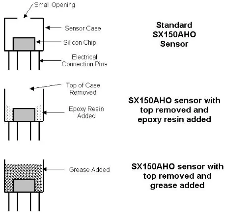
The stock SX150AHO sensor had a relatively small opening in its case, therefore the top of the case was removed in many instances to improve the filling time of the sensor (refer to figure 5.4. The filling time is the time taken for a higher pressure gas to fill the sensor.

[image:62.595.210.439.436.658.2]

Removing the top of the case further exposed the silicon diaphragm of the sensor to the test fluid. In these cases, to prevent foreign particles in the test gas from damaging the sensor, grease or latex were added (see figure 5.4) . Epoxy resin was also added to the sensors in some configurations to protect the gold connecting leads on the chip (the electrical connections). The use of Margarine (thinned with additional Canola oil) to protect the silicon chip was also trailed. This provided a readily available low viscosity grease-like compound, however Margarine was later found to deliver inconsistent results.

Figure 5.4: Modification of SX150AHO sensors

(63)

viewed in table 5.1.

Calibration Number Sensor Modification

1 Unmodified

2 Top of sensor removed

3 Top removed, Epoxy added around chip

(wires and diaphragm exposed)

4 Top removed, Epoxy added around chip

(wires covered, diaphragm exposed)

5 Sensor from (4), approx 1mm layer grease

added over diaphragm

6 Sensor from (5), approx 3mm layer grease

added over diaphragm (grease up to sensor lip)

7 Sensor from (2), thin layer latex (<1mm)

added over diaphragm

8 Sensor from (7), grease added up to sensor lip

over diaphragm

9 Sensor, top removed, approx 3mm of

Mar-garine added over diaphragm (up to sensor lip)

Table 5.1: Summary of sensor modifications used for shock tube tests

The analysis of the Shock Tube tests for each of the sensor configurations displayed in table 5.1 is detailed in the next section.

5.3

Analysis of Results

The summary shown in table 5.2 displays the type of sensor used for each Shock Tube test. The atmospheric pressure and temperature at the time of each test were also recorded to allow for analysis of the Shock Tube results. The MATLAB script associ-ated with the analysis of the Shock Tube tests, ’‘shock analysis2’ is shown in Appendix C.

(64)

Shock Test Number Related Calibration Notes 1 1 2 1 3 2 4 2 5 3 6 3 7 4 8 5

9 5 Sensor had approx 2mm layer grease

(cal. for 1mm layer of grease used)

10 6

11 7

added (cal. for no grease used)

14 8

15 8

16 9

17 9

Table 5.2: Shock Tube tests and corresponding sensors used

5.3.1 Reflected Shock Pressures

A theoretical analysis was used to calculate the fluid characteristics of the shock wave generated in the Shock Tube. This analysis, consisting of basic gas equations, was provided in a series of MATLAB scripts produced by Dr. David Buttsworth. The program code for running this analysis ’p T reflected’ is displayed in Appendix C.

By determining the inbound shock speed and inputting the ambient temperature and pressure, the reflected shock conditions of the test gas could be determined. This allowed the theoretical reflected shock pressure to be compared with the value indicated by the piezoresistive pressure transducer.

(65)

Shock Tube (173.5 mm in figure 5.2) (the distance between the second piezoelectric transducer and the piezoresistive transducer was therefore actually 176.5 mm). As the shock wave passed these sensors, a sudden increase in pressure occurred. A rapid increase in pressure also occurred in the piezoresistive pressure transducer (mounted at the end of the Shock Tube). By measuring the time between the sudden pressure changes in the sensors, the shock wave speed could be determined.

The measurement of shock speed between the three different sensors allowed three different shock speeds to be determined

-• Shock speed between the piezoelectric sensors

• Shock speed between the piezoelectric and piezoresistive sensor

• Estimated shock speed at the piezoresistive sensor

To estimate the shock speed at the piezoresistive sensor, a uniform deceleration of the shock wave was assumed. Therefore, given the time and location of the shock wave at the two piezoelectric sensors and the piezoresistive sensor, a third shock speed was calculated (the shock speed at the piezoresistive sensor). A second order polynomial was fitted to the points of time and displacement at each of the sensors. The gradient of this polynomial at the point of the piezoresistive sensor determined the shock speed at that point.

Since there was some degree of error in identifying the precise shock arrival times at each of the pressure transducer