This is a repository copy of Low Order Model for the Dynamics of Bi-Stable Composite Plates.
White Rose Research Online URL for this paper: http://eprints.whiterose.ac.uk/81015/
Version: Submitted Version
Article:
Arrieta, A.F., Spelsberg-Korspeter, G., Hagedorn, P. et al. (2 more authors) (Submitted: 2011) Low Order Model for the Dynamics of Bi-Stable Composite Plates. Journal of Intelligent Material Systems and Structures, 22 (17). 2025 - 2043. ISSN 1045-389X https://doi.org/10.1177/1045389X11422104
Reuse
Unless indicated otherwise, fulltext items are protected by copyright with all rights reserved. The copyright exception in section 29 of the Copyright, Designs and Patents Act 1988 allows the making of a single copy solely for the purpose of non-commercial research or private study within the limits of fair dealing. The publisher or other rights-holder may allow further reproduction and re-use of this version - refer to the White Rose Research Online record for this item. Where records identify the publisher as the copyright holder, users can verify any specific terms of use on the publisher’s website.
Takedown
If you consider content in White Rose Research Online to be in breach of UK law, please notify us by
Low order model for the dynamics of bi-stable
composite plates
Andres F. Arrieta∗, Gottfried Spelsberg-Korspeter, Peter Hagedorn
System Reliability and Machine Acoustics, Dynamics and Vibrations Group Technische Universit¨at Darmstadt, LOEWE-Zentrum AdRIA, Darmstadt, 64289
Germany
Simon A. Neild, David J. Wagg
Department of Mechanical Engineering,University of Bristol, Bristol, U.K, BS8 1TR
Abstract
This paper presents the derivation and validation of a low order model for the nonlinear dynamics of cross-ply bi-stable composite plates focusing on the response of one stable state. The Rayleigh-Ritz method is used to solve the associated linear problem to obtain valuable theoretical insight into how to formulate an approximate nonlinear dynamic model. This allows us to follow a Galerkin approach projecting the solution of the nonlinear problem onto the mode shapes of the linear problem. The order of the nonlinear model is reduced using theoretical results from the linear solution yielding the low order model. The dynamic response of a bi-stable plate specimen is studied to simplify further the model by only keeping the nonlinear terms leading to observed oscillations. Simulations for the dynamic response using the derived model are presented showing excellent agreement with the
exper-∗Corresponding author. Tel.:+4961517058324
imentally observed behaviour. Furthermore deflection shapes are measured and compared to the calculated mode shapes, showing good agreement. Key words: Bi-stable composites, Morphing structures, Low order modelling, Mode shapes
1. Introduction
Structures made from composite laminates are becoming increasingly important in a wide variety of applications including adaptive structures. Promising developments in this field relate to curved composite laminates which have multiple statically stable shapes [1]. These shapes result from an unsymmetric stacking sequence leading to asymmetric residual thermal stresses being induced during the curing process [2]. The transition between stable states is achieved by a snap-through mechanism which is strongly non-linear in nature [3]. Due to the property of multi-stability, these materials have been considered for use in a range of adaptive structures, particularly for morphing aerospace structures [4]. Recently, techniques to design the in-duced thermal stresses have allowed the production of a wide range of desired stable shapes [5], and aerospace applications using the designed morphing ca-pabilities have been proposed [6].
these composite structures to high levels of dynamic excitation, for example in an aeroelastic environment. Potentially, dynamic excitations could induce undesired sudden jumps between stable states or even early fatigue failure to the structure. However, to date, very little work has been carried out to examine the dynamics of bi-stable composites. A theoretical study of the dynamics of snap-through in bi-stable composites has been conducted [15]. It compared a semi-analytical model for the deflection of bi-stable compos-ites based on a strain energy approximation with Finite Element Analysis re-sults, showing good agreement for the force required to trigger snap-through. Experimentally, high amplitude oscillations of a bi-stable plate, showing in-dications of chaotic oscillations across the snap-through region, have been presented [16]. In addition, the nonlinear dynamic response of a single stable state of a bi-stable composite plate was experimentally studied showing the response is dominated by 1/2 subharmonic oscillations [17].
Experimental studies on the deflection of circular [21] and spherical isotropic plates [22] can be found in the literature. However, few studies comparing experimental deflection shapes to theoretical mode shapes were found in the literature [22]. To the knowledge of the authors no comparison between the-oretical mode shapes and experimental deflection shapes for bi-stable com-posites has been presented. A good understanding of the deflection shape of such structures is paramount in the successful implementation of morph-ing and vibration suppression control for structures incorporatmorph-ing bi-stable composite. The nonlinear problem is approximated by following a Galerkin procedure projecting the solution onto the mode shapes of the linear problem obtaining a set of nonlinear modal equations. Theoretical observations from the linear solution show close agreement between the chosen shape functions and the mode shapes obtained for the associated linear problem allowing to reduce the order of the nonlinear model. An experimental characterisation is conducted for the linear and nonlinear response of a square carbon-fibre epoxy bi-stable plate [04−904]T test specimen showing very close agreement
with the theoretical observations. In addition, this characterisation is used to retain the relevant nonlinear terms in the modal nonlinear equations of the low order model. A validation of the model is conducted by comparing simu-lated results for the key dynamic features of the response with experimental results.
using Love’s equations of motion for a shell including the von K´arm´an non-linearity in strain-displacement relations to account for geometric nonlinear-ities [26]. The Galerkin approach is followed to obtain a set of nonlinear ordinary differential equations using the shape functions employed in sec-tion 2 as a base for the expansion of the transverse displacement nonlinear solution. In section 3, the dynamic response of a test specimen is studied. Theoretical results are used to reduce the number of degrees-of-freedom and the required nonlinear terms to be kept in the equations to obtain a good low-order approximation for the dynamics of the plate, as described in section 4. In section 5, simulations for frequency response diagrams and displace-ment time series are conducted using the derived model showing good match with the experimental results. In section 6 of this paper, the mode shapes obtained in section 2 are compared to deflection shapes for the bi-stable plate specimen, showing good agreement. In addition, the deflection shapes for subharmonic oscillations are studied revealing a nonlinear behaviour in the spatial response. Finally, conclusions are presented and future research directions are discussed.
2. Model derivation
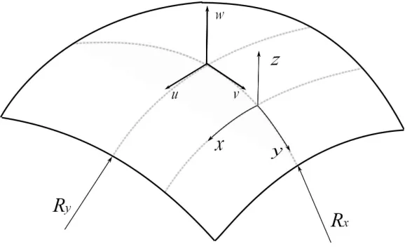
Figure 1: Curvilinear coordinates (x, y) and shell displacements u(x, y, t), y(x, y, t) and
w(x, y, t).
the model, first the associated linear problem is solved with the Rayleigh-Ritz method, allowing us to obtain mode shapes for the reduced nonlinear problem, as well as for comparison with experimentally measured deflection shapes. Secondly, a Galerkin procedure to approximate the solution of the nonlinear problem is conducted, using the same shape functions as for the Rayleigh-Ritz method to obtain nonlinear modal equations for the time re-sponse of cross-ply bi-stable composites.
2.1. Linear formulation
un-symmetrically laminated shell is given by
L = V − T, (1)
where L is the Lagrangian of the system. The strain (potential) energy is written as
Vs=
RLx
−Lx
RLy
−Ly
Nxxǫoxx+Nyyǫoyy+Nxyǫxyo +Mxxkxx+Myykyy+Mxykxy
dydx,
(2)
where Nij and Mij are the membrane forces and bending moments
respec-tively, and Lx and Ly are the dimensions of the shell (see Fig. 1). The
membrane and bending strains, ǫo and k respectively, are given by
ǫoxx =
∂u ∂x +
w Rx
, (3a)
ǫo yy =
∂v ∂y +
w Ry
, (3b)
ǫo xy =
∂u ∂y +
∂v
∂x, (3c)
(3d)
and
kxx = −
∂2w
∂x2, (4a)
kyy = −
∂2w
∂y2, (4b)
kxy = −2
∂2w
∂x∂y. (4c)
shallow composite shell [29], as
Nxx = A11ǫoxx+A12ǫyy+B11kxx,
Nyy = A21ǫoxx+A22ǫyy+B22kyy,
Nxy = A33ǫoxy,
Mxx = B11ǫoxx +D11kxx+D12kyy,
Myy = B22ǫoyy+D21kxx+D22kyy,
Mxy = D33kxy, (5a)
where Aij, Bij and Dij represent the membrane stiffnesses, coupling moduli
and the bending stiffnesses of coordinate i acting on the direction j respec-tively, and u(x, y, t), v(x, y, t) and w(x, y, t) are the displacements in the x,
y and z coordinate directions. An additional term in the strain energy is introduced to account for an elastic support to which the bi-stable plate may be attached to, given by
Vb =
1 2
Z Lx
−Lx
Z Ly
−Ly
kxu2+kyv2+kzw2
dxdy, (6)
where kx, ky and kz are the elastic constants of the support in x, y and z
directions [19]. The total strain energy is thus
V = Vs+Vb. (7)
The kinetic energy may be written as
T = 1
2ρh
Z Lx
−Lx
Z Ly
−Ly
h ˙
u2+ ˙v2+ ˙w2idxdy, (8)
The types of shells studied herein have unrestricted edges, i.e. free bound-ary conditions. Thus, no restrictions are placed on the admissible functions (shape functions) for the Rayleigh-Ritz procedure, as no geometric bound-ary conditions need to be satisfied. The solutions for the displacements along each coordinate direction are represented by the expansions
u(x, y, t) =
M X i=0 N X j=0
Uij(t)uij(x, y),
= I X i=0 J X j=0
Uij(t) cos
πxi Lx cos πyj Ly +
2I+1
X
i=I+1 2J
X
j=J+1
Uij(t) cos
πx(i−(I+ 1))
Lx
sin
πy(j−J)
Ly
+
3I+1
X
i=2I+2 3J+1
X
j=2J+1
Uij(t) sin
πx(i−(2I+ 1))
Lx
cos
πy(j−(2J+ 1))
Ly
+
4I+1
X
i=3I+2 4J+1
X
j=3J+2
Uij(t) sin
πx(i−(3I+ 1))
Lx
sin
πy(j−(3J+ 1))
Ly
,
v(x, y, t) = M X i=0 N X j=0
Vij(t)vij(x, y),
= I X i=0 J X j=0
Vij(t) cos
πxi Lx cos πyj Ly +
2I+1
X
i=I+1 2J
X
j=J+1
Vij(t) cos
πx(i−(I+ 1))
Lx
sin
πy(j−J)
Ly
+
3I+1
X
i=2I+2 3J+1
X
j=2J+1
Vij(t) sin
πx(i−(2I+ 1))
Lx
cos
πy(j−(2J+ 1))
Ly
+
4I+1
X
i=3I+2 4J+1
X
j=3J+2
Vij(t) sin
πx(i−(3I+ 1))
Lx
sin
πy(j −(3J+ 1))
Ly
,
(10)
w(x, y, t) =
M X i=0 N X j=0
Wij(t)wij(x, y),
= I X i=0 J X j=0
Wij(t) cos
πxi Lx cos πyj Ly +
2I+1
X
i=I+1 2J
X
j=J+1
Wij(t) cos
πx(i−(I + 1))
Lx
sin
πy(j−J)
Ly
+
3I+1
X
i=2I+2 3J+1
X
j=2J+1
Wij(t) sin
πx(i−(2I+ 1))
Lx
cos
πy(j−(2J + 1))
Ly
+
4I+1
X
i=3I+2 4J+1
X
j=3J+2
Wij(t) sin
πx(i−(3I+ 1))
Lx
sin
πy(j−(3J + 1))
Ly
,
(11)
whereUij(t),Vij(t) andWij(t) are time response coefficients to be determined,
uij(x, y), vij(x, y) and wij(x, y) are the shape functions on each coordinate
functions on each expansion as M ×N. Notice that the above given shape functions used to represent the displacements are all the possible non-zero combinations of sinusoidal functions. In addition to the constant term given by subscriptsi= 0j = 0, the two added terms inM = 4I+2 andN = 4J+2 account for the constants obtained from the cosine terms cos (0) multiplied by all the possible sine functions in each displacement direction.
Substituting Eqs. (9)-(11) into Eq. (1), and using Lagrange’s equations [30]
d dt
∂L
˙
qi
− ∂L
qi
= 0, (12)
where the generalized coordinatesqiare the time responses forming the vector
q = [Uij(t), Vij(t), Wij(t)]T, the equations of motion for the linear problem
are obtained by substituting q=keiωt in Eq. (12), written as
K−ω2M
k= 0. (13)
is attached to an elastic support, as is the case for any real specimen with free boundary conditions, for which the corresponding natural frequencies are non zero. Figs. 2(g)-2(l) show the first six flexible modes of the compos-ite plate. Each are either symmetric (S) or antisymmetric (A) with respect to the (x,y) axes of the shell, thus the notation for the first out-of-plane mode having symmetry with respect to the x-direction and antisymmetry with respect to the y-direction is (S, A)w
1. The corresponding mode shape for
mode (S, A)w
1 is w(S,A)1. The theoretical results obtained from Eq. (13) are
further exploited in section 4 to obtain a low order model for the dynamics of bi-stable composites.
2.2. Nonlinear analysis
To study the nonlinear response of bi-stable composites the classical shal-low shell nonlinear vibration theory is folshal-lowed. This takes into account the effect due to the curvature and the stretching of the middle surface cap-tured by the von-K´arm´an geometric nonlinearity in the strain-displacement relations [31], given by
ǫo xx =
∂u ∂x +
w Rx
+1 2
∂w ∂x
2
, (14a)
ǫo yy =
∂v ∂y +
w Ry
+ 1 2
∂w ∂y
2
, (14b)
ǫo xy =
∂u ∂y +
∂v ∂x+
∂w ∂x
∂w
∂y. (14c)
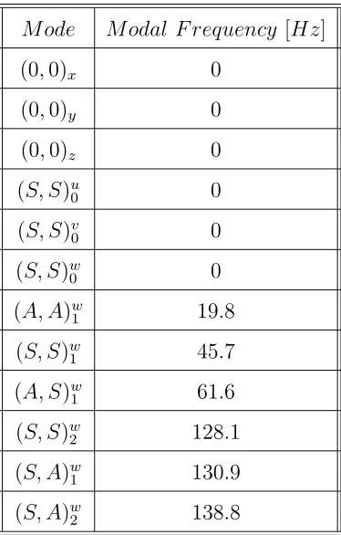
Mode Modal F requency [Hz]
(0,0)x 0
(0,0)y 0
(0,0)z 0
(S, S)u
0 0
(S, S)v
0 0
(S, S)w
0 0
(A, A)w
1 19.8
(S, S)w
1 45.7
(A, S)w
1 61.6
(S, S)w
2 128.1
(S, A)w
1 130.9
(S, A)w
[image:14.595.212.399.226.519.2]2 138.8
Table 1: Modal frequencies for the first 12 modes. Notice that the first 6 modes are rigid
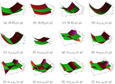
(a) (0,0)x(x, y) (b) (0,0)y(x, y) (c) (0,0)z(x, y) (d) u(S,S)0(x, y)
(e) v(S,S)0(x, y) (f) w(S,S)0(x, y) (g) w(A,A)1(x, y) (h) w(S,S)1(x, y)
[image:15.595.110.501.124.411.2](i)w(A,S)1(x, y) (j) w(S,S)2(x, y) (k) w(S,A)1(x, y) (l)w(S,A)2(x, y)
Figure 2: Mode shapes (deformed shapes) for the first 12 modes of a square cross-ply
bi-stable composite plate with unsymmetrical stacking sequence obtained with Eq. (13).
Figures 2(a)-2(c) show the rotational rigid body modes in the x-, y- and z-directions, and
Figs. 2(d)-Fig. 2(f) show the translational rigid body modes in the x-, y- and z-directions.
Flexural modes are shown in Figs. 2(g)-2(l) where the subscripts refer to the symmetry
class and the modal number for each mode shape, e.g. w(S,A)1 refers to the first
out-of-plane mode shape of the symmetric-antisymmetric symmetry class.
com-posite is given by [35]
(D11−P11B112 )
∂4w
∂x4 + 2(D12+P12B11B22+ 2D33)
∂4w
∂x2∂y2 + (D22−P22B 2 22)
∂4w
∂y4
+ 1
Rx
∂2φ
∂y2 +
1
Ry
∂2φ
∂x2 −
∂2φ
∂y2
∂2w
∂x2 −
∂2φ
∂x2
∂2w
∂y2 + 2
∂2w
∂x∂y ∂2φ
∂x∂y
+P12B11
∂4φ
∂y4 +P12B22
∂4φ
∂x4 −(P11B11+P22B22)
∂4φ
∂x2∂y2 +Cw˙ +ρhw¨=
p(x, y, t)−kzw(xs, ys, t),
(15)
where Rx and Ry are the radii of curvature in the x- and y-directions
re-spectively, C is the viscous damping, h is the thickness, ρ the density of the plate, kz is the stiffness of a support to which the plate may be attached,
and p(x, y, t) is the external excitation. For a detailed derivation see for example [33]. The coefficients Pij are given by
(P11, P12, P22) =
(A22, A12, A11)
A11A22−A212
, (16)
P33 =
1
A66
. (17)
The compatibility equation is obtained from the elasticity relations for a body subject to a state of plane stress [26], and may be written as
P11
∂4φ
∂y4 +P22
∂4φ
∂x4 + (P33−2P12)
∂4φ
∂x2∂y2 =P12B11
∂4w
∂x4 +P12B22
∂4w
∂y4
−(P11B11+P22B22)
∂4w
∂x2∂y2 +
1
Rx
∂2w
∂y2 +
1
Ry
∂2w
∂x2 + (
∂2w
∂x∂y)
2− ∂2w
∂x2
∂2w
∂y2,
(18)
where Airy’s stress function φ(x, y, t) is defined as
Nxx =
∂2φ
∂y2, Nyy =
∂2φ
∂x2, Nxy =−
∂2φ
(see for example [34]).
Equations (15) and (18) govern the dynamics of the transverse displace-ment of the bi-stable composite confined to one stable state, thus no changes between stable states or snap-through are accounted for. These equations are solved using a Galerkin approach, as outlined in [35]. Both the trans-verse displacement w(x, y, t) and the stress function φ(x, y, t) are defined in the same domain and therefore it is assumed that they can be expanded in the same shape functions w(i,j)(x, y). This is exact, for the case of a simply
supported plate with homogeneous material properties subject to small de-flections [36]. For the case being considered here, this is an approximation due to the coupling between in-plane and transverse deflections caused by the curvature and unsymmetrical lamination. However, for shallow shells this approximation yields very good results [41]. Therefore, the solution for the transverse displacement and stress functions are written as
w(x, y, t) =
N
X
i=0 N
X
j=0
w(i,j)(x, y)Wij(t), (20)
φ(x, y, t) =
N
X
m=0 N
X
n=0
w(m,n)(x, y)Fij(t), (21)
where wij(x, y) are the shape functions given in Eq. (11), and, W(i,j)(t) and
F(m,n)(t) are the displacement and stress function time response coefficients
for shape function (i, j) and (m, n), the parenthesis in the equations for time responses W(i,j)(t) and F(m,n)(t) are dropped for clarity. Note that the
first term in Eq. (20), i, j = 0, corresponds to a purely rigid body transla-tion of the bi-stable plate in the out-of-plane directransla-tion, given by the term cosπx0
Lx
cosπyL0
y
rota-tional rigid body modes with respect to the in-plane directions also result in out-of-plane displacements of the bi-stable plate. For the case where the studied composite is attached to an elastic support as the one described in Eq. (6), these rigid body modes will have a non-zero modal frequency. It is assumed that the torsional rigidity of the support is large, thus only the translational mode (S, S)w
0 is considered in the derivation neglecting the
ro-tational modes (0,0)x, (0,0)y and (0,0)z.
to obtain N X i=0 N X j=0 h
(D11−P11B112 )w
′′′′
ij (x, y) + (D22−P22B222 )wij∗∗∗∗(x, y)
i
Wij(t)
+ N X i=0 N X j=0
2(D12+P12B11B22+ 2D33)w
′′∗∗
ij (x, y)Wij(t)
+ N X m=0 N X n=0 1 Ry
w′′mn(x, y) +
1
Rx
w∗∗
mn(x, y)
Fmn(t)
+ N X m=0 N X n=0 h
P12B11w
′′′′
mn(x, y) +P12B22w∗∗∗∗mn (x, y)
i
Fmn(t)
− N X m=0 N X n=0
(P11B11+P22B22)w
′′∗∗
mn(x, y)Fmn(t)− N X i=0 N X j=0 N X m=0 N X n=0 h
(wij′′(x, y)w∗∗
mn(x, y) +w∗∗ij(x, y)w ′′
mn(x, y)
i
Wij(t)Fmn(t)
+ N X i=0 N X j=0 N X m=0 N X n=0 h 2w′∗
ij(x, y)w ′∗ mn(x, y)
i
Wij(t)Fmn(t)
+ N X i=0 N X j=0
wij(x, y)CijW˙ij + N X i=0 N X j=0
wij(x, y)ρhW¨ij =p(x, y, t)− N X i=0 N X j=0
kzwij(x, y)Wij
and N X m=0 N X n=0 h
P22w
′′′′
mn(x, y) +P11wmn∗∗∗∗(x, y) + (P33−2P12)w
′′∗∗ mn(x, y)
i
Fmn(t)
= N X i=0 N X j=0 1 Ry
wij′′(x, y) + 1
Rx
w∗∗
ij(x, y)
Wij(t)
+ N X i=0 N X j=0 h
P12B11w
′′′′
ij (x, y) +P12B22wij∗∗∗∗(x, y)
i
Wij(t)
− N X i=0 N X j=0 h
(P11B11+P22B22)w
′′∗∗ ij (x, y)
i
Wij(t)
+ N X i=0 N X j=0 N X p=0 N X q=0 h
w′∗
ij(x, y)w ′∗
pq(y)−w ′′
ij(x, y)wpq∗∗(x, y)
i
Wij(t)Wpq(t),
(23)
where{}∗and{}′indicate differentiation with respect toxandyrespectively
and the summation indices m, n have been used for φ, and, i, j and p, q for the cases where w is multiplied by another w term. Following the Galerkin procedure a set of modal nonlinear equations is obtained by projecting the solution onto shape functions given in Eq. (11), leading to a system of two coupled nonlinear equations of dimension 2(N ×N) each. This is achieved by multiplying Eq. (22) by arbitrary shape functions w(a,b), and Eq. (23)
by arbitrary shape functions w(m,n), integrating over the surface of the shell
and using the orthogonality conditions of the shape functions, given in Ap-pendix B, to obtain
¨
Wab+ 2ζab,plateωab,plateW˙ab+ωab,plate2 Wab+ ([Γab] + [Ξab])Fab
+ N X k=0 N X l=0 N X p=0 N X q=0 h
and
Fmn= [Gmn]−1([Hmn] + [Nmn])Wmn+ N X i=0 N X j=0 N X p=0 N X q=0
[Gmn]−1
Tmnijpq
WijWpq,
(25)
where [G], [H], [N], [T], [Γ], [Π] and [Ξ] are coefficients depending on the mode shapes, Qab is the modal participation factor for mode (a, b) due to the
external forcing, Kz
ab is the stiffness term due to the elastic support in the
z-direction, and, ωab,plate and ζab,plate are the natural frequency and damping
ratio without including the curvature effect for mode (a, b). The definition of the coefficients multiplying the time response functions for the deflection W
and stress function F in Eqs. (22) and (23) are given in Appendix B. Notice that since the shape functions for both the transverse displacement and the stress functions are sinusoidal functions, the stress function time response is decoupled from the transverse displacement in Eq. (25). This allows us to decouple the system of equations and write the governing equation of motion for the transverse displacement by substituting the expressions for F(m,n) in
Eq. (24) as
¨
Wab+ 2ζabωabW˙ab+ω2abWab
+ N X i=0 N X j=0 N X p=0 N X q=0
[Gab]−1([Γab] + [Ξab])
Tabijpq
WijWpq
+ N X i=0 N X j=0 N X m=0 N X n=0
[Gab]−1([Hab] + [Nab]) Π ijpq ab
WijWab
+ N X i=0 N X j=0 N X p=0 N X q=0 N X m=0 N X n=0
[Gab]−1
Tabijpq Πijmnab
WijWpqWab =Qab− KzabWab,
whereωab andζab are the natural frequency and damping ratio including the
curvature effects, accounted by term [Gab]−1([Γab] + [Ξab]) ([Hab] + [Nab]), for
mode (a, b). Equation (26) gives the modal equation for the time response
Wab of mode (a, b), including all possible modal interactions. The solution
for the time response coefficients along with the corresponding mode shapes, are substituted in Eq. (20) to obtain the solution for the transverse nonlinear vibration of a bi-stable composite.
3. Dynamic response
The dynamics of a test specimen are experimentally studied to identify the existence of important nonlinear phenomena in the response of the bi-stable plate following the procedure detailed in Ref. [17]. These results allow for identifying nonlinear oscillations of the tested plate as well as to validate the derived model, as detailed in section 5. A bi-stable composite plate with unsymmetric stacking sequence [04−904]T and dimension 300 by 300 mm is
used as the specimen for this study. The radii of curvature of the specimen
Rx and Ry are 0.9 m and 10 m, respectively. The material properties of
the specimen are given in Table 2. A schematic diagram of the plate in the stable configuration studied throughout this paper is shown in Fig. 3. In this state, the x-direction and y-direction are aligned with the larger and smaller curvatures of the plate, i.e. with the directions of principal curvature. The measured points Px and Py lie just off lines crossing at centre of the plate
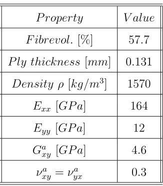
P roperty V alue
F ibrevol. [%] 57.7
P ly thickness [mm] 0.131
Density ρ [kg/m3] 1570
Exx [GP a] 164
Eyy [GP a] 12
Ga
xy [GP a] 4.6
νa
[image:23.595.224.387.122.308.2]xy =νyxa 0.3
Table 2: Material properties for a ply of HexPly 8557 IM7 used to manufacture the
bi-stable plate experimental specimen.
the edges are unrestrained, resulting in a plate with free boundary conditions attached to an elastic support.
Figure 3: Measured points to study the out-of-plane displacement of the bi-stable plate.
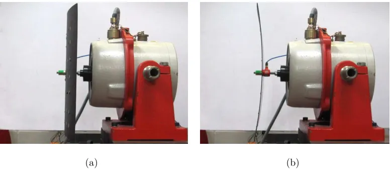
[image:23.595.182.426.425.603.2](a) (b)
Figure 4: Bi-stable plate mounted on Ling shaker, which is used as external excitation
source. (a) Stable state 1. (b) Stable state 2. (Reproduced with the kind permission of
the Journal of Intelligent Material Systems and Structures [39])
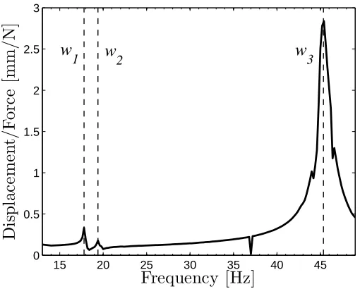
amplitude response of the specimen in the frequency range of interest for this work. This is chosen so it contains the frequencies for which snap-through is achieved with less actuation effort [39]. The FRF for pointPx for
a low forcing amplitude of 1 N shows a linear response for this low level of excitation in Fig. 5. Three modes dominate the response of the specimen in this frequency range: mode w1 at 17.6 Hz, mode w2 at 19.4 Hz and mode
w3 at 45.4 Hz. Comparing the obtained theoretical modal frequencies with
the experimental results it is observed that mode w2 and w3 correspond
to theoretical modes (A, A)w
1 and (S, S)w1, respectively. A distinct notation
between theoretical modes (e.g. (S, S)w
0) and experimental modes (e.g. w1),
will be used throughout the paper for differentiation. Mode w1 does not
relate to theoretical flexible modes, however inspecting its deflection shape, shown in Fig. 9(a), it corresponds to the rigid body translational mode in the out-of plate direction (S, S)w
frequency is not zero as the plate is attached to an elastic support. This effect is taken into account by introducing a non-zero stiffness in the out-of-plane direction, kz, in Eq. (6), the remaining elastic constants kx and ky are zero.
15 20 25 30 35 40 45
0 0.5 1 1.5 2 2.5 3
Frequency [Hz]
D
is
p
lac
em
en
t/F
or
ce
[m
m
/N] w
2 w3
w
[image:25.595.170.425.209.414.2]1
Figure 5: Experimental receptance (Displacement/Force) FRF for point Px. Forcing
am-plitudeFo = 1.0N, frequency range Ω=[13,49]
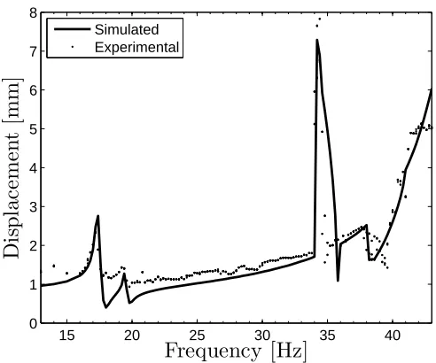
signalling nonlinear oscillations. The experimental frequency response dia-gram measured at point Px for an input force amplitude of 5 N is shown
in Fig. 6. The response is qualitatively similar to that observed in the lin-ear FRF in Fig. 5, except for the regions around 35 Hz and 39 Hz. The multiple points shown in the experimental frequency response diagram in Fig. 6 indicate the appearance of nonlinear oscillations for these frequency ranges. Inspecting the time series for the deflection of point Px presented
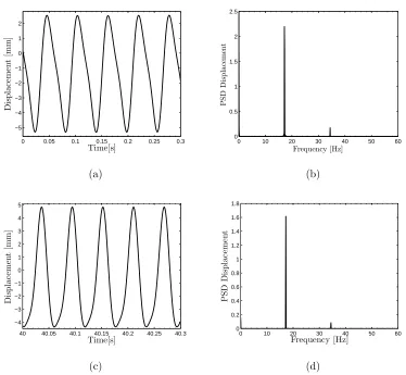
in Fig. 7(a) for a forcing frequency of 34.4 Hz, we observe a non-sinusoidal response to a harmonic excitation of the plate. The power spectrum of this time response is presented in Fig. 7(b). It shows that most of the energy transmitted by the external forcing at 34.4 Hz, is transferred to a lower fre-quency at around 17.6 Hz. This frefre-quency is very close to the experimentally identified modal frequency for mode w1. The experimental observations for
this nonlinear response show that as the forcing frequency is increased, the expected linear type response at the forcing frequency loses its stability. A completely different solution showing harmonics at the modal frequency and at twice the modal frequency (coinciding with the forcing frequency) appear around these frequency ranges. These characteristics match those of 1/2 subharmonic oscillations of mode w1 [17, 40].
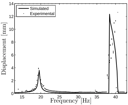
A similar behaviour can be seen for the experimental frequency response diagram measured at pointPy for the response of modew2, shown in Fig. 8. A
dominant nonlinear response is seen around 39 Hz, this is at twice the modal frequency of modew2. This response was previously observed in Fig. 6,
15 20 25 30 35 40 0
1 2 3 4 5 6 7 8
Frequency [Hz]
D
is
p
lac
em
en
t
[m
m
]
[image:27.595.178.424.135.340.2]Simulated Experimental
Figure 6: Experimental frequency response diagram for point Px. Fo=5.0 N, frequency
range Ω=[13,43]
the experimental results agree with the characteristics of a 1/2 subharmonic response of modew2. Although other sub- and super- harmonics were
exper-imentally searched for, both at lower and higher frequencies, no others could be found for the chosen levels of forcing and the current plate configuration.
4. Low order model formulation
The main focus of this work is to develop a low order model for the trans-verse nonlinear dynamics of bi-stable composites confined to a stable state. Inspecting results from the associated linear eigenvalue problem, Eq. (13), it is noticed that very few shape functions are required to almost completely span the subspace of the first few transverse displacement eigenvectors. In particular, for the transverse displacement modes (A, A)w
vir-0 0.05 0.1 0.15 0.2 0.25 0.3 −5 −4 −3 −2 −1 0 1 2 Time[s] D is p lac em en t [m m ] (a)
0 10 20 30 40 50 60 0 0.5 1 1.5 2 2.5 Frequency [Hz] P S D D is p la ce m en t (b)
40 40.05 40.1 40.15 40.2 40.25 40.3 −4 −3 −2 −1 0 1 2 3 4 5 Time[s] D is p lac em en t [m m ] (c)
[image:28.595.115.489.126.471.2]0 10 20 30 40 50 60 0 0.2 0.4 0.6 0.8 1 1.2 1.4 1.6 1.8 Frequency [Hz] P S D D is p lac em en t (d)
Figure 7: Experimental and simulated dynamic response for pointPx. Forcing amplitude
Fo=5N, forcing frequency Ω=34.4Hz. (a) Experimental displacement time response. (b)
Experimental displacement power spectrum. (c) Simulated displacement time response.
(d) Simulated displacement power spectrum.
tually no coupling exists between in-plane and transverse terms. Further-more, for these modes it is possible to closely approximate each mode shapes with only one shape function. Therefore, it is possible to treat these shape functions as eigenvectors of transverse displacement for modes (A, A)w
1, and
(S, S)w
15 20 25 30 35 40 0
2 4 6 8 10 12 14
Frequency [Hz]
D
is
p
lac
em
en
t
[m
m
]
[image:29.595.173.424.135.340.2]Simulated Experimental
Figure 8: Experimental frequency response diagram for pointPy. Measured using
strobo-scopic sampling for a forcing amplitude ofFo= 5.0N, frequency range Ω=[13,43]
Fig. 2(f), is also closely approximated by a constant given by cosines terms in Eq. (11) and the shape function w(S,S)1. These theoretical results allow for
truncating the number of terms used in the nonlinear problem solution, keep-ing only the relevant terms givkeep-ing the eigenvectors of modes (S, S)w
0, (A, A)w1,
and (S, S)w
1, i.e shape functions w(S,S)0, w(A,A)1, and w(S,S)1. Moreover, the
previous discussion leading to an order reduction of the derived nonlinear model corresponds closely to the results from the dynamic characterisation presented in section 3. Thus, the solution for the transverse displacement
w given by Eq. (20) can be truncated keeping only the first three shape functions in the expansion, i.e. w(0,0),w(1,1) andw(1,0)corresponding to
solution for the transverse displacement is thus written as
w(x, y, t) =
N
X
i=0 N
X
j=0
(w(0,0)+w(1,0))W00(t) +w(1,1)W11(t) +w(1,0)W10(t)
wij(x, y)Wij(t),
(27) where W(0,0)(t), W(1,1)(t) and W(1,0)(t), and, w(0,0)(x, y), w(1,1)(x, y), and
w(1,0)(x, y) are the time response coefficients and mode shapes for
theoreti-cal modes (S, S)w
0, (A, A)w1, and (S, S)w1 respectively. Following the Galerkin
procedure by substituting Eq. (27) into Eq. (26), integrating over the shell domain, and dropping vanishing coefficients, the following nonlinear ordinary differential equations are obtained
¨
W00+ 2ζ00wω00wW˙00+ω
2
00wW00+ Φ
00w
1110W11W10+ Φ000000W00W00+
Φ001100W11W00+ Φ000010W00W10+ Φ001111W11W11+ Φ00100110W10W01W10+
Φ00110110W11W01W10+ Φ00110110W11W01W10+ Φ00111110W11W11W10=Q00sin (Ωt),
(28)
¨
W11+ 2ζw11ωw11W˙11+ω
2
w11W11+ Φ
11
1001W10W01+ Φ011011W10W11+
Φ111101W11W01+ Φ111111W11W11+ Φ10011111 W10W01W11+ Φ11110111W11W01W11+
Φ10
101111W10W11W11+ Φ11111111W11W11W11=Q11sin (Ωt),
(29)
¨
W10+ 2ζw10ωw10W˙10+ω
2
w10W10+ Φ
10
1110W11W10+ Φ101001W10W01+
Φ101101W11W01+ Φ101010W10W10+ Φ101111W11W11+ Φ10100110W10W01W10+
Φ10110110W11W01W10+ Φ10110110W11W01W10+ Φ10111110W11W11W10=Q10sin (Ωt),
where the coefficients Φ are calculated using Eq. (26) and the relations given in Appendix B, andωw00,ωw11 andωw10 are the theoretical modal frequencies
of modes (S, S)w
0, (A, A)w1, and (S, S)w1 respectively.
To reduce the nonlinear terms in Eqs. (28)-(30), the experimental obser-vations for the response of the plate are employed. First, only interactions between experimental modes w1 and w3, and modes w2 and w3, which
cor-respond to theoretical modes (S, S)w
0 and (A, A)w1, with mode (S, S)w1 are
experimentally observed. Thus, all terms leading to other modal interactions are dropped. Second, only 1/2 subharmonic oscillations of modes w1 andw2
were observed in the response. Therefore, quadratic terms alone are kept in the equations to account for this dominant nonlinear response [42, 43, 44], al-lowing us to neglect cubic terms which lead to 1/3 sub- and super-harmonic oscillations not observed for the current configuration. This last simplifi-cation agrees with previous theoretical and experimental studies of shells, where cubic terms have been neglected as the quadratic terms arising from the curvature dominate the response of such structures [22]. Finally, the values of the nonlinear coefficients remaining in the governing equations are identified from the experimental frequency response diagrams.
Now we can rewrite equation Eqs. (28)-(30) for a sinusoidal forcing in the centre of the plate to obtain the reduced set nonlinear modal equations as
¨
W00+ 2ζw1ωw1W˙00+ω
2
w1W00+α11W
2
00+α13W00W10=Q00sin(Ωt), (31)
¨
W11+ 2ζw2ωw2W˙11+ω
2
w2W11+α22W11
2+α
23W11W10=Q11sin(Ωt), (32)
¨
W10+ 2ζw3ωw3W˙10+ω
2
w3W10 =Q10sin(Ωt), (33)
for mode w1 with natural frequency ωw1 = 17.6 Hz, W(1,1)(t) is the time
response coefficient of the transverse displacement for mode w2 with natural
frequency ωw2 = 19.4 Hz, W(1,0)(t) is the time response coefficient of the
transverse displacement for mode w3 with natural frequency ωw3 = 45.4 Hz,
Ω is the forcing frequency, Qij is the modal participation factor for mode
wi given in Appendix B, αij is the coefficient for the nonlinear quadratic
term for an interaction between modes (wi, wj). The system of reduced
Eqs. (31)-(33) gives the time response for the set of modes kept in the low order model. These equations are solved numerically to obtain simulated modal time functions for the transverse deflection. The complete solution is obtained by substituting the modal time functions along with the associated mode shapes obtained from Eq. (13), into Eq. (20).
5. Simulations and model validation
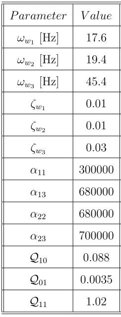
The reduced set of nonlinear equations for the modal time responses given by Eqs. (31)-(33) are solved using a Runge-Kutta type solver. The coeffi-cients for the equations of motion are identified using experimental frequency response diagrams obtained as detailed in section 3. The parameters used in the simulations for equations Eqs. (31)-(33) are given in Table 3. The numerical solution for the reduced set of equations in the derived model is used to calculate the simulated dynamic response of the bi-stable plate and compared to the experimental results. The simulated frequency response di-agram for point Px is presented in Fig. 6 in a solid line and compared with
P arameter V alue
ωw1 [Hz] 17.6
ωw2 [Hz] 19.4
ωw3 [Hz] 45.4
ζw1 0.01
ζw2 0.01
ζw3 0.03
α11 300000
α13 680000
α22 680000
α23 700000
Q10 0.088
Q01 0.0035
[image:33.595.243.365.124.442.2]Q11 1.02
Table 3: Parameters used in numerical simulations.
comparing the displacement and power spectrum graphs of point Px for a
forcing frequency Ω of 34.4 Hz, given in Figs. 7(c)-7(d), with the experimen-tal results, shown in Figs. 7(a)-7(b), the ability of the model to capture even detailed dynamic features is highlighted. In addition, a comparison between the experimental and simulated frequency response diagrams for point Py is
shown in Fig. 8. As for point Px, a close quantitative and qualitative match
6. Spatial response comparison
Experimental deflection shapes are obtained and compared to theoretical mode shapes. The experimental deflection shapes are obtained by exciting the plate with sinusoidal inputs for a forcing frequency equal to the frequency of the relevant modes. Additionally, deflection shapes for the ranges of sub-harmonic oscillations are also obtained. The measurements are performed for a range of forcing amplitudes between [0.5,5] N in both stable states for each of the dominant modes and subharmonic oscillations in order to detect possible amplitude dependent deflection shapes. The experimental results for both stable states are virtually identical, and for illustration we use those obtained for state one. A Polytec OFV056/3001 scanning laser vibrometer is used to acquire instant displacement for a grid of point on the bi-stable plate surface. The software provided by the laser vibrometer manufacturer is used to construct the deflection shapes. The algorithm obtains amplitude and phase information for each point on the grid. The displacement in space of these points is measured with respect to a plane (shown as a squared grid in Figs. 9(a), 9(b), 10(a), 10(b), 11(a), 11(b), 12 and 13), from which the deflected shapes can be inferred based on the assumption that the static curvature is small (see section 2 and Fig. 1).
Figures 9(a) and 9(b) show the experimental and simulated mode shapes for mode w1. Comparing the measured deflection shape shown in Figs. 9(a)
(a) (b)
[image:35.595.109.496.118.518.2](c) (d)
Figure 9: Comparison between experimental deflections shapes for mode w1 and mode
shapes obtained from Eq. (13) for mode (S, S)w
0. (a) 3-D view of the experimental
deflec-tion shape for modew1. (b) Lateral view (ZXplane) of the experimental deflection shape
for mode w1. (c) 3-D view of simulated mode shape (deformed shapes)w(S,S)0(x, y). (d)
Lateral (ZX plane) view of simulated mode shape (deformed shapes)w(S,S)0(x, y).
ob-tained, however no amplitude dependent behaviour is observed, hence these images are omitted. The mode shapes and the experimental deflection shapes for modes w2 and w3 are also compared in Figs. 10 and 11, respectively. For
mode w2 the experimental deflection shape differs from the calculated mode
shape. The observed mismatch may be explained by the effects added by the non perfect support and small geometrical imperfections in the shape of shells, as a non-uniform curvature, which can largely alter the actual shape of the deflection [22, 31]. For mode w3 very good agreement between the
measured deflection shape and calculated mode shape is achieved as seen in Fig. 11. This is a very relevant result since this mode dominates the dy-namic behaviour in the frequency range of interest, which potentially allows us to use the model for morphing shape and vibration suppression control of bi-stable composites.
The deflection shapes for the subharmonic oscillations are also studied. Figure 12 shows the deflection shape for a forcing amplitude of 1 N and a forcing frequency of 34.8 Hz. For this level of forcing no subharmonic response is observed (see Fig. 12), thus the measured shape matches that observed for mode w3 as it dominates the linear response in this range of
frequencies. As the forcing amplitude is increased and the subharmonic in-stability is triggered, the plate response shows two dominant harmonics, at the forcing frequency and at half the forcing frequency. The corresponding deflection shapes are shown in Figs. 13(a) and 13(b). In view of this, the actual deflection shape for the subharmonic response is assumed to be the sum of the linear response dominated by mode w3, and the response due
(a) (b)
[image:37.595.111.495.110.508.2](c) (d)
Figure 10: Comparison between experimental deflections shapes for mode w2 and mode
shapes obtained from Eq. (13) for mode (A, A)w
1. (a) 3-D view of the experimental
de-flection shape for mode w2. (b) Lateral view (ZY plane) of the experimental deflection
shape for modew2. (c) 3-D view of simulated mode shapew(A,A)1(x, y). (d) Lateral (ZY
plane) view of simulated mode shapew(A,A)1(x, y).
(a) (b)
[image:38.595.109.495.107.506.2](c) (d)
Figure 11: Comparison between experimental deflections shapes for mode w3 and mode
shapes obtained from Eq. (13) for mode (S, S)w
1. (a) 3-D view of the experimental
deflec-tion shape for modew3. (b) Lateral view (ZXplane) of the experimental deflection shape
for modew3. (c) 3-D view of simulated mode shapew(S,S)1(x, y). (d) Lateral (ZXplane)
view of simulated mode shapew(S,S)1(x, y).
Figure 12: Experimental deflection shape for a forcing frequency of 34.8 Hz
respect to the x-direction deviating from the deflection shape of w1, as can
be seen by comparing Figs. 9(a) and 13(a). Hence, as the subharmonic oscil-lations are triggered, the deflection shape of the plate varies, resulting in an amplitude dependent behaviour of the spatial response. In spite of this, the measured nonlinear deflection shape behaviour is approximated by the model with the chosen mode shapes obtained from the associated linear problem, as explained in the following.
The time response of modeW(0,0) when the subharmonic oscillations are
triggered is non-zero, this condition can be written as
W(0,0) = 0, f or F0 < Fsubw1
W(0,0) 6= 0, f or F0 ≥Fsubw1
(34)
where F0 is the forcing amplitude, and Fsubw1 is the forcing amplitude
re-quired to trigger the subharmonic oscillations for mode w1 previously
subhar-monic oscillations associated to mode w1 is given by
w1sub(x, y, t) = (w(0,0)+w(1,0))W00(t) +w(1,0)W10(t), (35)
as the response for W(1,1) is negligible for this frequency range. The total
response for the subharmonic oscillations associated to mode w2 can be
ob-tained following a similar procedure using the results for Fsubw2 given in [17].
Equation (35) shows the ability of the derived model to qualitatively approx-imate the observed nonlinear deflection shape behaviour.
[image:40.595.124.485.309.457.2](a) (b)
Figure 13: Experimental deflection shape for a subharmonic response. Forcing amplitude
Fo=4 N, forcing frequency Ω=34.8 Hz. (a) Experimental deflection shape due to the
response content at 17.6 Hz. forcing frequency of 34.8 Hz. (b) Experimental deflection
shape due to the response content at 34.8 Hz.
7. Conclusions
the full response for the transverse displacement following a Rayleigh-Ritz-Galerkin approach. The number of modes in the general model is reduced based on theoretical results from the associated linear problem to obtain a low order model for the dynamics of bi-stable composites. The reduced model is validated comparing simulated results to the experimental response of a bi-stable plate test specimen. The experimentally observed subharmonic oscillations are modelled accurately with the nonlinearities kept in the low order model. In addition, the calculated modal frequencies from the asso-ciated linear problem are in good agreement with the experimental results providing an upper frequency bound for each mode.
Acknowledgements
The authors would like to acknowledge the support of the ORS scheme; Andres F. Arrieta was funded through an ORS scholarship during the time of this research. In addition, the authors would like to thank Dr. Anirvan DasGupta for his invaluable remarks and Dr. Dario Di Maio for his help to obtain the experimental deflection shapes.
A. Components of the mass and stiffness matrices
The mass matrix M in Eq. (13) is given by
Maijmn [0] [0]
[0] Mbijmn [0]
[0] [0] Mcijmn
, (A.1)
where the coefficients are
Maijmn = ρh
Z Lx
0
Z Ly
0
(uijumn)dydx, (A.2)
Mbijmn = ρh
Z Lx
0
Z Ly
0
(vijvmn)dydx, (A.3)
Mcijmn = ρh
Z Lx
0
Z Ly
0
(wijwmn)dydx. (A.4)
The stiffness matrix Kin Eq. (13) is given by
Ku
aijmn Kbijmnu Kcijmnu
Ku
bijmn Kbijmnv Kcijmnv
Ku
cijmn Kcijmnv Kcijmnw
where the coefficients are written as
Kaijmnu =
Z Lx
0
Z Ly
0
A11(u∗iju∗mn) +A33(u′iju′mn)
dxdy, (A.6)
Kbijmnu =
Z Lx
0
Z Ly
0
A12(u∗ijvmn∗ ) +A33(u′ijvmn∗ )
dxdy, (A.7)
Kcijmnu =
Z Lx
0
Z Ly
0 A11 u∗ ij wmn Rx +A12
u∗ ij wmn Ry
−B11 u∗ijwmn∗∗
dxdy
(A.8)
Kbijmnv =
Z Lx
0
Z Ly
0
A22(v′iju′mn) +A33(vij∗vmn∗ )
dxdy, (A.9)
Kcijmnv =
Z Lx
0
Z Ly
0 A22 v′ ij wmn Ry +A12
v′ ij wmn Rx
−B22 vij′ w′′mn
dxdy
(A.10)
Kcijmnw =
Z Lx
0
Z Ly
0
(A11
wij
wmn
Rx
+A22
wij
wmn
Ry
+ 2A12
wijwmn
RxRy
−B11
wijw∗∗mn
Ry
−B22
wijwmn∗∗
Ry
+D11 wij∗∗w∗∗mn
+D22 w′′ijwmn′′
+ 2D12 wij∗∗w′′mn
+ 4D33
w∗′ ijw∗
′ mn
+kzwijwmn)dxdy.(A.11)
B. Orthogonality conditions and coeffients
The orthogonality conditions for sinusoidal functions used in Eqs. (25)-(26) are given by
Z L
0
sin(αmx) sin(αnx) =
0, f or m6=n
L
2, f or m =n
(B.1)
Z L
0
cos(αmx) cos(αnx) =
0, f or m6=n
L
2, f or m =n
Z L
0
sin(αmx) cos(αnx) = 0. (B.3)
The coefficients used in Eqs. (25)-(26) are given by
Kzab =
kz ω2 ab,plateρh , (B.4) ω2 ab,plate = 1 ρh λ 4
xa D11−P11B
2 11
+λ4
yb D22−P22B
2 22
+ 1
ρh2λ
2 xaλ
2
xb(D12+P12B11B22+ 2D33), (B.5)
ω2ab=ωab,plate2 +Kz
ab+ [Gab]−1([Γab] + [Ξab]) ([Hab] + [Nab]) (B.6)
ζab,plate =
Cab
ω2
ab,plateρh
, (B.7)
ζab =
Cab
ω2 abρh
, (B.8)
Γab =
1 ρh 1 Rx γ2 yb +
1 Ry γ2 xa , (B.9)
Ξab =
1
ρh γ
4
ybP12B11+γ
4
xaP12B22+γ
2 xaγ
2
yb(P11B11+P22B22)
,
(B.10)
Πijmnab = 1
LxLyρh
−λ2xaγy2nΦijmnab −γ2xaλy2nΦijmnab + 2λxiλyjγxmγynΦ
ijmn ab
,
(B.11)
Gab =
LxLy
4 γ
4
xaP11+γ
4
ybP22+γ
2 xaγ
2
yb(P33−2P12)
, (B.12)
Hab =
LxLy
4
1
Rx
λ2xa+
1
Ry
λ2ya
Nab =
LxLy
4 λ
4
xaP12B11+λ
4
ybP12B22−λ
2 x1λ
2
xb(P11B11+P22B22)
, (B.14)
Tabijmn = λxiλyjγxmγynΦ
ijmn ab +λ
2 xiγ
2 ynΦ
ijmn ab
, (B.15)
Qab =
4
LxLyρh
Z Lx
0
Z Ly
0
p(x, y, t)Xa(x)Yb(y)dydx, (B.16)
λxa =
πxa Lx
, (B.17)
γxa =
πxa Lx
, (B.18)
where the coefficients Φ is defined as
Φijmnab =
Z Lx
0
Z Ly
0
w(a,b)(x, y)w(i,j)(x, y)w(m,n)(x, y)dydx, (B.19)
References
[1] M.-L. Dano, M.W. Hyer, Thermally-induced deformation behavior of unsymmetric laminates. International Journal of Solids and Structures, 35, (1998) 2101-2120.
[2] M. Schlecht, K. Schulte, Advanced calculation of the room-temperature shapes of unsymmetric laminates, Journal of Composite Materials, 33. (1999) 1472-1490.
[3] S.V. Sokorin, A.V. Terentiev, On Modal Interaction, Stability and Non-linear Dynamics of a Model Two D.O.F. Mechanical System Performing Snap-Through Motion, Nonlinear Dynamics, 16, (1998) 239-257.
[5] K. Potter, P.M. Weaver, A concept for the generation of out-of-plane distortion from tailored FRP laminates, Composites Part A, 35, (2004) 1353-1361.
[6] C. G. Diaconu, P. M. Weaver, F. Mattioni, Concepts for morphing airfoil sections using bi-stable laminated composite structures, Thin-Walled Structures, 46, (2008) 689-701.
[7] F. Mattioni, P.M. Weaver, K. Potter, M.I. Friswell, The application of residual stress tailoring of snap-through composites for variable sweep wings, Proceedings of the 47th AIAA/ASME/ASCE/AHS/ASC Struc-tures, Structural Dynamics, and Materials Conference, Rhode Island, May (2006).
[8] M.-L. Dano, M.W. Hyer, Snap-through of unsymmetric fiber-reinforced composite laminates. International Journal of Solids and Structures, 39, (2002) 175-198.
[9] W. Hufenbach, M. Gude, L. Kroll, Design of multistable composites for application in adaptive structures, Composites Science and Technology, 62,(2002) 2201-2207.
[10] P. Giddings, C.R. Bowen, R. Butler, H.A. Kim, Characterisation of actu-ation properties of piezoelectric bi-stable carbon-fibre laminates, Com-posites Part. A, 39,(2008) 697-703.
[12] M.-L. Dano, M.W. Hyer, SMA-induced snap-through of unsymmetric fiber-reinforced composite laminates,International Journal of Solids and Structures, 40, (2003) 5949-5972 .
[13] K. Potter, P. Weaver, A.A. Seman, S. Shah, Phenomena in the bifur-cation of unsymmetric composite plates. Composites Part A, 35,(2006) 100-106.
[14] M.R Schultz, M.W. Hyer, R.B. Williams, W.K. Wilkie, D.J. Inman, Snap-through of unsymmetric laminates using piezocomposite actua-tors, Composite Science and Technology, 66, (2006) 2442-2448.
[15] C. G. Diaconu, P. M Weaver, A. F. Arrieta, Dynamic analysis of bi-stable composite plates, Journal of Sound and Vibration, 22, (2009) 987-1004.
[16] A.F. Arrieta, F. Mattioni, S.A. Neild, P.M. Weaver, D.J. Wagg, K. Pot-ter, Nonlinear dynamics of a bi-stable composite laminate plate with ap-plications to adaptive structures, Proceedings of the 2nd European Con-ference for Aero-Space Sciences(EUCASS2007), Brussels, July (2007)
[17] A. F. Arrieta, S.A. Neild, D.J. Wagg, Nonlinear dynamic response and modelling of a bi-stable composite plate for applications to adaptive structures, Nonlinear Dynamics, 58, (2009) 259-272.
[19] K. M. Liew and K. Y. Lam, Effects of Arbitrarily Distributed Elas-tic Point Constraints on Vibrational Behaviour of Rectangular Plates, Journal of Sound and Vibration, 174, (1994) 23-36.
[20] S. Hurlebaus, L. Gaul, J. T.-S. Wang. An exact series solution for cal-culating the eigenfrequencies of orthotropic plates with completely free boundarys, Journal of Sound and Vibration, 244, (2001) 747-759.
[21] O. Thomas, C. Touze, A. Chaigne, Asymmetric non-linear forced vibra-tions of free-edge circular plates. part ii: experiments. Journal of Sound and Vibration, 265, (2003) 1075-1101.
[22] O. Thomas, C. Touze, E Luminais, Non-linear vibrations of free-edge thin spherical shells: Experiments on a 1:1:2 internal resonance, Non-linear Dynamics, 49, (2007) 259-284.
[23] A.H. Nayfeh, D.T. Mook, Nonlinear Oscillations. Wiley, New York, (1979).
[24] S. Lefschetz, Modern Mathematics for the Engineer. Mcgraw-Hill, New York, (1956).
[25] T. Von Karman, The Engineer Grapples With Nonlinear Problems. Bul-letin of American Mathematical Society, 46,(1940) 615-683.
[26] A.H. Nayfeh, P.F. Pai, Linear and Nonlinear Structural Mechanics. Wi-ley, New York, (2004).
[28] P. Hagedorn and A. DasGuptaVibration and Waves in Continuous Me-chanical Systems. John Wiley & Sons, Chichester, (2007).
[29] A.H. Nayfeh, Introduction to Composite Materials, Technomic Publish-ing Company, Inc., Lancaster, (1980).
[30] L. MeirovitchMethods of Analytical Dynamics. McGraw-Hill, New York, (1970).
[31] M. Amabili, Nonlinear Vibrations and Stability of Shells and Plates, Cambridge University Press, (2008).
[32] V. Z. Vlasov, Basic differential equations in the general theory of elastic shells, NACA TM 1241, 1951.
[33] D.J. Wagg, S.A. Neild, Nonlinear vibration with control: for flexible and adaptive structures, Springer, (2009).
[34] W. Nowacki, Dynamics of Elastic Systems, Wiley, (1963).
[35] C.-Y. Chia, Nonlinear Analysis of Plates, McGraw-Hill, (1980).
[36] A.W. Leissa, Vibration of Shells, National Aeronautics and Space Ad-ministration, (1971).
[37] A.W. Leissa, Free vibration of rectangular-plates, Journal of Sound and Vibration, 31, (1973) 257-293.
[39] A. F. Arrieta, D.J. Wagg, S.A. Neild, Dynamic snap-through for morph-ing of bi-stable composite plates,Journal of Intelligent Material Systems and Structures, in Press, (2010).
[40] A.H. Nayfeh, Nonlinear Interactions, Analytical, Computational, and Experimental Methods, Wiley, New York, (2000).
[41] W. Soedel, Vibration of shells and plates, Marcel Dekker, Inc., (2004).
[42] B. Balachandran, A.H. Nayfeh, Observations of Modal Interactions in Resonantly Forced Beam-Mass Structures, Nonlinear Dynamics, 2, (1991) 77-117.
[43] S.H. Chen, Y.K. Cheung, H.X. Xing, Nonlinear Vibration of Plane Structures by Finite Element and Incremental Harmonic Balance Method, Nonlinear Dynamics, 26, (2001) 87-104.