This is a repository copy of
Long-distance quantum key distribution with imperfect devices
.
White Rose Research Online URL for this paper:
http://eprints.whiterose.ac.uk/78176/
Version: Published Version
Article:
Lo Piparo, N and Razavi, M (2013) Long-distance quantum key distribution with imperfect
devices. Physical Review A: Atomic, Molecular and Optical Physics, 88 (1). 012332. ISSN
1050-2947
https://doi.org/10.1103/PhysRevA.88.012332
eprints@whiterose.ac.uk https://eprints.whiterose.ac.uk/ Reuse
Unless indicated otherwise, fulltext items are protected by copyright with all rights reserved. The copyright exception in section 29 of the Copyright, Designs and Patents Act 1988 allows the making of a single copy solely for the purpose of non-commercial research or private study within the limits of fair dealing. The publisher or other rights-holder may allow further reproduction and re-use of this version - refer to the White Rose Research Online record for this item. Where records identify the publisher as the copyright holder, users can verify any specific terms of use on the publisher’s website.
Takedown
If you consider content in White Rose Research Online to be in breach of UK law, please notify us by
Long-distance quantum key distribution with imperfect devices
Nicol´o Lo Piparo and Mohsen Razavi*
School of Electronic and Electrical Engineering, University of Leeds, Leeds, United Kingdom
(Received 5 November 2012; published 30 July 2013)
Quantum key distribution over probabilistic quantum repeaters is addressed. We compare, under practical assumptions, two such schemes in terms of their secret key generation rates per quantum memory. The two schemes under investigation are the one proposed by Duanet al.[Nature (London)414, 413 (2001)] and that of Sangouardet al.[Phys. Rev. A76, 050301 (2007)]. We consider various sources of imperfection in both protocols, such as nonzero double-photon probabilities at the sources, dark counts in detectors, and inefficiencies in the channel, photodetectors, and memories. We also consider memory decay and dephasing processes in our analysis. For the latter system, we determine the maximum value of the double-photon probability beyond which secret key distillation is not possible. We also find crossover distances for one nesting level to its subsequent one. We finally compare the two protocols in terms of their achievable secret key generation rates at their optimal settings. Our results specify regimes of operation where one system outperforms the other.
DOI:10.1103/PhysRevA.88.012332 PACS number(s): 03.67.Bg, 03.67.Dd, 03.67.Hk, 42.50.Ex
I. INTRODUCTION
Despite all practical progress with quantum key distribution (QKD) [1–4], its implementation over long distances remains to be a daunting task. In conventional QKD protocols such as BB84 [5], channel loss and detector noises set an upper bound on the achievable security distance [6]. In addition, the path loss results in an exponential decay of the secret key generation rate with distance. Both of these issues can, in principle, be overcome if one implements entanglement-based QKD protocols [7,8] over quantum repeater systems [9–12]. This approach, however, is not without its own challenges. Quantum repeaters require quantum memory (QM) units that can interact with light and can store their states for sufficiently long times. Moreover, highly efficient quantum gates might be needed to perform two-qubit operations on these QMs [9]. The latter issue has been alleviated, to some extent, by introducing a novel technique by Duan, Lukin, Cirac, and Zoller (DLCZ) [10], in which initial entanglement distribution and swapping, thereafter, rely on probabilistic linear-optic operations. Since its introduction, the DLCZ idea has been extended and a number of new proposals have emerged [13–18]. Such probabilistic schemes for quantum repeaters particularly find applications in QKD systems of mid- to long distances, which makes them worthy of analytical scrutiny. This paper compares DLCZ with one of its favorite successors [17], which relies on single-photon sources (termed SPS protocol, hereafter). Using a general system-level approach, which encompasses many relevant physical sources of imperfections in both systems, we provide a realistic account of their performance in terms of their secret key generation rates per logical memory used. This measure not only quantifies performance, but it also accounts for possible costs of implementation.
The SPS protocol attempts to resolve one of the key drawbacks in the original DLCZ protocol: multiphoton emis-sions. DLCZ uses atomic ensembles as QMs, which lend themselves to multiphoton emissions. This leads to obtaining not fully entangled states, hence resulting in lower key
*m.razavi@leeds.ac.uk
rates when used for QKD. To tackle this issue, in the SPS protocol, entanglement is distributed by ideally generating single photons, which will either be stored in QMs or directed toward a measurement site. Whereas, in principle, the SPS protocol should not deal with the multiphoton problem, in practice, it is challenging to build on-demand single-photon sources that do not produce any multiphoton components. A fair comparison between the two systems is only possible when one considers different sources of nonidealities in both cases, as we pursue in this paper.
The SPS protocol is one of the many proposed schemes for probabilistic quantum repeaters. In [18] authors provide a review of all such schemes and compare them in terms of the average time that it takes to generate entangled states, of a certain fidelity, between two remote memories. Their conclusion is that in the limit of highly efficient memories and detectors, the top three protocols are the SPS protocol and two others that rely on entangled and two photon sources [14,16]. In more practical regimes, however, the SPS protocol seems to have the best performance per memory and/or mode used. In this paper, we therefore focus on the SPS protocol and investigate, under practical assumptions, whether the above conclusion remains valid in the context of QKD systems.
Our work is distinct from previous related work in its focusing on the performance of QKDsystems over quantum repeaters. In [18], authors have adopted the general measure of fidelity to find the average time of entanglement generation. Whereas their approach provides us with a general insight into some aspects of quantum repeater systems, it cannot be directly applied to the case of QKD. In the latter, the performance is not only a function of the entanglement generation rate, but also the quantum bit error rate caused by using nonideal entangled states. To include both of these issues, here we adopt the secret key generation rate per memory as the main figure of merit, by which we can specify the optimal setting of the system and its performance in different regimes of operation.
our analysis, we provide a normalized key rate per memory and/or mode. We calculate the dependence of the secret key generation rate on different system parameters when resolving or nonresolving detectors are used. In particular, we find the optimal values for relevant system parameters if loss, double-photon emissions, and dark counts are considered. Moreover, we account for the dephasing and the decay of memories in our analysis. Memory decoherence is one of the key challenges in any practical setup.
The paper is structured as follows. In Sec.II, we review the DLCZ and the SPS protocols, their entanglement distribution and swapping schemes, as well as their QKD measurements. In Sec.III, we present our methodology for calculating the secret key generation rate for the SPS protocol, followed by numer-ical results in Sec.IV. We draw our conclusions in Sec.V.
II. TWO PROBABILISTIC SCHEMES FOR QUANTUM REPEATERS
In this section we review two probabilistic schemes, namely, DLCZ and SPS, for quantum repeaters. We describe the multiple-memory setup for such systems and model relevant system components.
A. DLCZ entanglement-distribution scheme
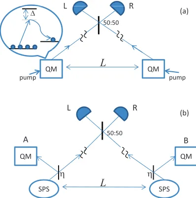
The DLCZ scheme works as follows [see Fig. 1(a)]. Ensemble memories A and B, at distance L, are made of atoms with -level configurations. They are all initially in their ground states. By coherently pumping these atoms, some of them may undergo off-resonant Raman transitions that produce Stokes photons. The resulting photons are sent toward a 50:50 beam splitter located at distanceL/2 between
L R
L R
50:50
(a)
QM QM
pump pump
L
L R
50:50
(b)
QM QM
A B
L
SPS
L
SPSFIG. 1. (Color online) Schematic diagram for entanglement distribution between quantum memories (QMs)AandBfor (a) the DLCZ protocol and (b) the SPS protocol. In both cases, we assume QMs can store multiple excitations. Sources, memories, and detectors are represented by circles, squares, and half circles, respectively. Vertical bars denote beam splitters. In both protocols the detection of a single photon ideally projects the two memories onto an entangled state.
A and B. If, ideally, only one photon has been produced in total at the ensembles, one and, at most, only one of the detectors in Fig. 1(a) clicks. In such a case, the DLCZ protocol heralds A and B to be ideally in one of the Bell states |ψ±AB=(|10AB± |01AB)/
√
2, where |0J is the
ensemble ground state and |1J =SJ†|0J is the symmetric
collective excited state of ensembleJ =A, B,where SJ† is the corresponding creation operator [10]. An important feature of such collective excitations is that they can be read out by converting their states into photonic states.
The fundamental source of error in the DLCZ scheme is the multiple-excitation effect, where more than one Stokes photon are produced [11]. If the probability of generating one Stokes photon is denoted bypc, there is a probabilityp2c that each
ensemble emits one photon. If this happens, a click on one of the two detectors heralds entanglement generation, whereas the memories are in the separable state|11AB.
In practice, one has to find the right balance between the heralding probability, which increases with pc, and the
quantum bit error rate (QBER), which also increases withpc.
In [11], authors find the optimal value ofpc that maximizes
the secret key generation rate in various scenarios when photon-number resolving detectors (PNRDs) or nonresolving photon detectors (NRPDs) are used. In this paper, we use their results in our comparative study.
B. SPS entanglement-distribution scheme
The SPS protocol, proposed in [17] aims at reducing multiphoton errors and, in particular, terms of the form |11AB by using single-photon sources. The architecture of
this scheme is presented in Fig.1(b). The two remote parties each have one single-photon source and one memory. In the ideal scenario, each source produces exactly one photon on demand, and these photons are sent through identical beam splitters with transmission coefficientsη.It can be shown that the state shared by the QMs after a single click on one of the detectors in Fig.1(b)is given by [17]
η|00AB00| +(1−η)|ψ±ABψ±|, (1) which has our desired entangled state plus a vacuum compo-nent. The latter, at the price of reducing the rate, can be selected out once the above state is measured at later stages [10,11].
[image:3.608.72.271.455.657.2]L R L R
50:50 c
D
50:50
s s
D
c
(a) (b)
c c
L
A A’ B’ B
FIG. 2. (Color online) (a) Entanglement connection between two entangled linksA-A′andB′-B. The memoriesA′andB′are read out and the resulting photons are combined on a 50:50 beam splitter. A click on one of the detectors projectsAandBinto an entangled state. The retrieval efficiencies and quantum efficiencies are represented by fictitious beam splitters with transmission coefficient ηc and ηD,respectively. (b) The equivalent butterfly transformation to the measurement module, whereηs =ηcηD.
Throughout the paper, we assume that both setups in Fig.1 are symmetric and phase stabilized. Furthermore, all conditions required for a proper quantum interference at 50:50 beam splitters are assumed to be met. Recent experimental progress in QKD shows that it is indeed possible to achieve these conditions [22,23].
C. Entanglement swapping and QKD measurements
Figure 2(a) shows the entanglement swapping setup for the DLCZ and the SPS protocols. Entanglement is established between QM pairsAA′andB′Busing either protocol. A partial Bell-state measurement (BSM) on photons retrieved from the middle QMsA′andB′is then followed, which, upon success, leavesAandBentangled. The BSM is effectively performed by a 50:50 beam splitter and single-photon detectors. To include the effects of the atomic-to-photonic conversion efficiency and the photodetectors’ quantum efficiency, we introduce two fictitious beam splitters with transmission coefficients ηc and ηD, respectively. All photodetctors in
Fig.2 will then have unity quantum efficiencies. Note that the parameterηcalso includes the memory decay during the
storage time.
Figure2(b)provides a simplified model for the measure-ment module in Fig.2(a). The 50:50 beam splitter and the two fictitious beam splitters in Fig.2(b) constitute what we call abutterflyoperation, which is further studied in Sec.IIIand AppendixA.
Alice and Bob use two butterfly operations to generate a raw key bit, as shown in Fig.3. After generating entangled pairs over a distanceL, Alice and Bob retrieve the states of memories and perform a QKD measurement on the resulting photons. They apply a random relative phase shift,ϕ,of either 0 or π/2 between their two fields. They later, at the sifting stage, keep only data points where the same phase value is used by both parties. They then turn their sifted keys into a secret key by using privacy amplification and error reconciliation techniques. Eavesdroppers can be detected by following the BBM92 or the Ekert protocol [7,24].
As mentioned in Sec. I, previous analyses only provide the fidelity or the time required for a successful creation of an entangled state [17]. Instead, in Sec.III, we calculate the
3 3
50:50 c
c
D
D
50:50 c
c
D
D entangled
A
C
B
D
D c D
L
C D
FIG. 3. (Color online) QKD measurements on two entangled pairs. Two pairs of memories,A-BandC-D, each share an entangled state. Memories are read out and the resulting photons are combined at a beam splitter and then detected. Different QKD measurements can be performed by choosing different phase shift values,ϕ, of 0 andπ/2.
secret key generation rate for the SPS scheme and compare it with that of the DLCZ protocol reported in [11].
It is worth noting that because of the reliance of our QKD protocols on entanglement, all entanglement swapping operations at the middle nodes can be done by untrusted parties, e.g., service providers. This is, in essence, similar to the recently proposed measurement-device-independent QKD (MDI-QKD) protocols [25–27], which also rely on entanglement swapping. MDI-QKD schemes, in their original form, are not suitable for long-distance quantum cryptography. By combining them with quantum repeaters in a hybrid setup that relies on MDI-QKD for the access network and on quantum repeaters for the core network, one can achieve the best of the two worlds. Preliminary analysis on such hybrid networks has been done [28] and the extended work is in preparation.
D. Multiple-memory configuration
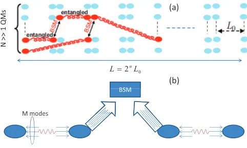
In order to compare different quantum repeater setups, we consider the multiple-memory configuration shown in Fig.4(a)
along with the cyclic protocol described in [29,30]. In this protocol, in every cycle of duration L0/c, where L0 is the
length of the shortest segment in a quantum repeater and c
(a) ( )
>1Q
M
s
N
BSM 0
2 L
L n
(b)
BSM
M modes M modes
>
[image:4.608.315.556.69.127.2] [image:4.608.75.271.72.163.2] [image:4.608.314.555.505.650.2]is the speed of light in the channel, we try to entangle any unentangled pairs of memories at distanceL0.We assume our
entanglement-distribution protocol succeeds with probability
PS(L0). At each cycle, we also perform as many BSMs as
possible at the intermediate nodes. The main requirement for such a protocol is that, at the stations that we perform BSMs, we must be aware of establishment of entanglement over links of lengthl/2 before extending it tol(informedBSMs). We use the results of [29] to calculate the generation rate of entangled statesper memoryin the limit of infinitely many memories. It is given byRent(L)=PS(L/2n)P
(1)
M P
(2)
M · · ·P
(n)
M /(2L/c),where
PM(i), i=1, . . . ,n,is the BSM success probability at nesting levelifor a quantum repeater withnnesting levels.
We use the following procedure, in forthcoming sections, to find the secret key generation rate of the setup in Fig.4(a). For each entanglement distribution scheme, we find PS(L0)
and relevantPM probabilities to deriveRent(L).We then find
the sifted key generation rate by multiplying Rent(L) by the
probability,Pclick,that an acceptable click pattern occurs upon
QKD measurements. Finally, the ratio between the number of secure bits and the sifted key bits is calculated using the Shor-Preskill lower bound [31]. In the limit of an infinitely long key, the secret key generation rate per logical memory is lower bounded by
RQKD(L)=max{Rent(L)Pclick[1−2H(ǫQ)],0}, (2)
whereǫQdenotes the QBER, andH(p)= −plog2p−(1−p)
log2(1−p),for 0p1.
E. Multimode-memory configuration
Another way to speed up the entanglement generation rate is via using multimode memories [15,32]. As can be seen in Fig.4(b), in this setup, we use only one physical memory per node but each memory is capable of storing multiple modes. In each round, we attempt to entangle memories at distance
L0 by entangling, at least, one of the existing M modes.
Once this occurs, we stop entanglement generation on that leg and wait until a BSM can be performed. For readout, all modes must be retrieved in order to perform BSMs or QKD measurements on particular modes of interest. In effect, this scheme is similar to that of Fig.4(a), except that entanglement distribution is not sequentially applied to unentangled modes. The success probability for entanglement distribution between the two memories is, however,Mtimes that of Fig.4(a). One can show that, the generation rate of entangled states per mode is approximately given by (23)nR
ent(L) [18,30].
In our forthcoming analysis, we consider only the case of Fig.4(a), but our results are extensible to the case of Fig.4(b)
by accounting for the relevant prefactor.
F. Memory decay and dephasing
Quantum memories are expected to decay and dephase while storing quantum states. In this paper, we model these two decoherence processes independently. The decay process, with a time constant T1, can be absorbed in the retrieval
efficiency of memories. If the retrieval efficiency immediately after writing into the memory is given byη0, after a storage time T, the retrieval efficiency is given by ηc=η0exp(−T /T1).
Different memories in the multiple-memory setup of Fig.4(a)
undergo different decay times. In our analysis, we consider the worst-case scenario, where all memories have decayed for
T =L/c, which is applicable only to the far-end memories. Under this assumption,ηccan be treated as a constant at all
stages of entanglement swapping.
We model the memory dephasing via a dephasing channel, by which the probability of dephasing after a period T is given by ed =[1−exp(−T /T2)]/2. In the context of the
QKD protocol in Fig. 3, this phase error is equivalent to the misalignment error in a conventional polarization-based BB84 protocol and has mostly the same effect. In our analysis, we neglect the effect of dephasing at the middle stages and consider only its effect on the far-end memories used for the QKD protocol. Again, for the multiple-memory setup of Fig.4(a), the relevant storage time is given byT =L/c[29].
III. SPS SECRET KEY GENERATION RATE
In this section, the secret key generation rate for the SPS scheme proposed in [17] is calculated. As shown in Sec.II, this scheme relies on simultaneous generation of single photons in two remote sites. Most practical schemes for the generation of single photons, however, suffer from the possibility of multiple-photon emissions. To address this issue, in this section we consider nonideal photon sources with nonzero probabilities for two-photon emissions and find the secret key generation rate in the repeater and no-repeater cases.
Suppose our photon sources emit one photon with proba-bility 1−pand two photons with probabilityp.We therefore have the following input density matrix for the initial state of
landrsources in Fig.5(a):
ρlr(in)=ρl(in)⊗ρr(in), (3) where
ρj(in)≡(1−p)|1jj1| +p|2jj2|, j =l, r. (4)
As we show later, in a practical regime of operation,
p≪1; hence, in our following analysis, we neglectO(p2)
terms corresponding to the simultaneous emission of two photons by both sources.
A. No-repeater case
In this section, we describe how we obtain parameters
PS, Pclick, and RQKD for the setup in Fig. 5(a) and QKD
measurements as in Fig.3.
Figure 5(a) depicts the entanglement-distribution setup for the SPS scheme. In our model the memories’ writing efficiencies, the path loss, and the detectors’ efficiencies are represented by fictitious beam splitters with transmis-sion coefficients ηm, ηt, and ηD, respectively, where ηt =
exp[−L/(2Latt)], with Latt=25 km for an optical fiber
channel. Photodetectors, in Fig.5, are then assumed to have unity quantum efficiencies.
In our analysis, we use an equivalent setup, as shown in Fig.5(b), where beam splitters have been rearranged such that
ηtηD =ηmηd.We can then recognize similar building blocks,
D
D d d
L R L R
(a) (b)
50:50
t
50:50
B B
A A
QM t QM QM QM
m
m m m m
m
r
r l
l SPS SPS SPS SPS
FIG. 5. (Color online) A schematic model for the SPS scheme. In (a) the memories’ writing efficiencies, the path loss, and the detectors’ efficiencies are represented by fictitious beam splitters with transmission coefficients ηm, ηt andηD, respectively. In (b), an equivalent model is represented, where we have grouped beam splitters in the form of butterfly modules; see Fig.6. Here,ηtηD= ηmηdand the model is valid so long asηtηdηm.
building block consisting of three beam splitters. For an input stateρL′R′in Fig.6, we denote the output state on portsLand
RasBηB,ηx(ρL′R′).
We use well-known models for beam splitters [33] to find output density matrices for input states to a generic butterfly module. In Appendix A, we find the relevant input-output relationships for the states of interest. We useMAPLE15 to simplify some of our analytical results. We can then find
ρALBR,the joint state of the memories and the optical modes
entering detectorsLandRin Fig.5(b)by applying the butterfly operation three times, as follows:
ρALBR=B0.5,ηd
Bη,ηm
ρl(in)⊗Bη,ηm
ρr(in). (5) According to the SPS protocol, a click on exactly one of the detectors L or R in Fig. 5(b)would herald the success of entanglement distribution. This process can be modeled by applying proper measurement operators considering whether PNRDs or NRPDs are used. For example, for a click on detectorL, the explicit form of the measurement operator is given by
M=
⎧
⎪ ⎪ ⎪ ⎨
⎪ ⎪ ⎪ ⎩
(1−dc)[|1LL1| ⊗ |0RR0|
+dc|0LL0| ⊗ |0RR0|], PNRD
(1−dc)[(IL− |0LL0|)⊗ |0RR0|
+dc|0LL0| ⊗ |0RR0|], NRPD
(6)
R
L
x
L’
R’
x
B
FIG. 6. (Color online) A generic butterfly module, represented by BηB,ηx,whereηBandηxare transmissivities for beam splitters shown in the figure.
whereIL denotes the identity operator for the mode entering
the left detector [34], anddc is the dark count rate per gate
width per detector.
After the measurement, the resulting joint state,ρAB,of
quantum memories is given by
ρAB=
trL,R(ρALBRM)
P , (7)
where
P =tr(ρALBRM)=
PS(L)
2 (8)
is the probability that the conditioning eventM occurs. The last equality is due to the symmetry assumption.
For QKD measurements, we assume that two pairs of memories, A-B and C-D, are given in an initial state similar to that of Eq. (7). We use the scheme described in Fig. 3 to perform QKD measurements. For simplicity, we assume both users use zero phase shifts; other cases can be similarly worked out in our symmetric setup. In Fig. 3, the retrieval efficiency and the quantum detectors efficiency are represented by fictitious beam splitters with, respectively, transmission coefficient ηc and ηD. It is again possible to
remodel the setup in Fig. 3 as shown in Fig.2(b) and use the butterfly operationB0.5,ηs, whereηs=ηcηD.The density
matrix right before photodetection in Fig.3is then given by
B0.5,ηs(B0.5,ηs(ρAB⊗ρCD)),where one of theB operators is
applied to modes A andC, and the other one to modes B
andD.Using this state, we findPclick andǫQas outlined in
AppendixB.
Using Eq.(2), the secret key generation rate per memory,
RQKD, in the no-repeater setup, is then lower bounded by [11] R1 =max
[1−2H(ǫQ)]
PS(L)
2L/c Pclick/2,0 , (9)
where PS(L)
2L/c, given by Eq. (8), is the generation rate of
entangled pairs per logical memory, Pclick is the probability
of creating a sifted key bit by using two entangled pairs, and [1−2H(ǫQ)] is the probability of creating a secret key bit out
of each sifted key bit. Here, we assume a biased basis choice to avoid an extra factor of two reduction in the rate [35]. The full definition forPclickis given by Eq.(B3). The QBER,
ǫQ=
Perror
Pclick
, (10)
where Perror is the probability that Alice and Bob assign
different bits to their sifted keys, is given by Eq.(B4).
B. Repeater case
First, consider the repeater setup of nesting level one in Fig. 2(a). We use the structure of Fig. 5(a) to distribute entanglement betweenA-A′andB′-B memories. The initial joint state of the system,ρAA′BB′=ρAA′⊗ρBB′,can then be
[image:6.608.53.292.73.191.2] [image:6.608.55.296.537.716.2]operators in Eq.(6), which results in
ρAB=
trLR(MρALBR′ )
PL
, (11)
whereρ′
ALBR =B0.5,ηs(ρAA′BB′), whereLandRrepresent the
input modes to the photodetectors. Note that in Fig. 2 the detectors have ideal unity quantum efficiencies. Moreover,
PL=tr(MρALBR′ )=PM/2 (12)
is the probability that only the left detector clicks in the BSM module of Fig. 2. A click on the right detector has the same probability by symmetry.
In order to find the secret key generation rate, we follow similar steps to the no-repeater case. That is, we apply the butterfly operation to find relevant density matrices, from which Pclick and ǫQ can be obtained. From Eq. (2), in the
one-node repeater case,RQKDis lower bounded by
R2 =max
[1−2H(ǫQ)]
PS(L/2)
2L/c PMPclick/2,0 . (13)
Using the same approach, and by using Eq.(2), we find the secret key generation rate for higher nesting levels. The details of which have, however, been omitted for the sake of brevity.
IV. NUMERICAL RESULTS
In this section, we present numerical results for the secret key generation rate of the SPS protocol, versus different system parameters, in the no-repeater and repeater cases, and we compare them with that of the DLCZ protocol. As mentioned earlier, we have used MAPLE 15 to analytically derive expressions for Eqs.(2),(9), and(13)when PNRDs or NRPDs are used. Unless otherwise noted, we use the nominal values summarized in TableIfor all the results presented in this section.
A. SPS key rate versus system parameters
1. Source transmission coefficient
Figure7shows the secret key generation rate per memory,
[image:7.608.312.557.72.208.2]RQKD, versus the source transmission coefficientηin Fig.1(b),
TABLE I. Nominal values used in our numerical results.
Memory writing efficiency,ηm 0.5 Quantum efficiency,ηD 0.3 Memory retrieval efficiency,ηc 0.7 Dark count per pulse,dc 10−6 Attenuation length,Latt 25 km
Speed of light,c 2×10⁵km/s
Decay (dephasing) time constants,T1(T2) ∞
0 0.1 0.2 0.3 0.4 0.5 0.6 0.7 0.8 0.9 1
0 1 2 3 4 5
x 10−4
Source transmission coefficient, η
Secret key generation rate per memory (b/s/QM)
0 0.5 1
0 2 4x 10 PS
0 0.5 1
0 0.005 0.01
Pclic
k
no−repeater PNRD no−repeater NRPD repeater PNRD repeater NRPD
η
FIG. 7. (Color online) RQKD versus the source transmission
coefficient η for the PNRDs and NRPDs in the no-repeater and one-node repeater cases. Here,p=0.001,L=250 km, andn=1 for the repeater system; other parameters are listed in TableI
atp=0.001 andL=250 km. It can be seen that there exist optimal values ofηfor both repeater and no-repeater systems. TableIIsummarizes these optimum values for different nesting levels. The optimal value of η for the no-repeater system is higher than the repeater ones, and that is because of the additional entanglement swapping steps in the latter systems. Another remarkable feature in Fig. 7 is that the penalty of using NRPDs, versus PNRDs, seems to be minor atp=10−3.
PNRDs better show their advantage at higher values ofpwhen double-photon terms become more evident.
The existence of an optimal value forηarises from a com-petition between the probability of entanglement distribution
PS, which grows withη,andPclick,which decreases withη.
This has been demonstrated in the inset of Fig.7. The latter issue is mainly because of the vacuum component in Eq.(1). In the case of the repeater system,PM also decreases withη
for the same reason, and that is why the optimal value ofηis lower for repeater systems.
The optimum values ofηin Fig.7are interestingly almost identical to the value ofηthat minimizes the total time for a successful creation of an entangled state, as prescribed in [17]. It is because, at a fixed distance, the QBER term in Eqs.(9)
and(13)is mainly a function of the double-photon probability and the dark count rate, and it does not vary considerably with
[image:7.608.47.295.664.751.2]η. More generally, the optimum values ofηremain constant as in TableIIso long as the error terms are well below the cutoff threshold in QKD.
TABLE II. Optimal values ofη, atp=0.001 andL=250 km, for repeater and no-repeater systems, when PNRDs or NRPDs are used. The figures with an asterisk are approximate values.
Nesting level PNRD NRPD
0 0.35 0.34
1 0.28 0.27
2 0.21 0.20*
[image:7.608.312.558.679.752.2]0 500 1000 1500 2000 2500 3000 10−12
10−10 10−8 10−6 10−4 10−2 100
Distance, L (km)
Secret key generation rate per memory (b/s/QM
)
two nesting levels three nesting levels one nesting level no repeater 0 500 1000 1500 2000 10
10 10
Key rate (b/s/QM)
d
c = 0
d
c = 10 −7
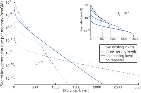
FIG. 8. (Color online) RQKD versus distance for up to three
nesting levels at two different dark count rates atp=10−4. All other
values are listed in TablesIandII.
2. Nesting levels and crossover distance
Figure8depicts the normalized secret key generation rate versus distance for different nesting levels. At dc=0, the
slope advantage, proportional toPS(L/2n), for higher nesting
levels is clear in the figure. Because of additional entanglement swapping stages, the no-path-loss rate atL=0 is, however, lower for higher nesting levels. That would result in crossover distances—at which one system outperforms another—once we move from one nesting level to its subsequent one. The crossover distance has architectural importance and will specify the optimum distance between repeater nodes.
The crossover distance is a function of various system parameters. As shown in the inset of Fig. 8, positive dark count rates can change considerably the crossover distance. By including dark counts in our analysis, there will be a cutoff security distance for each nesting level. By increasing the dark count rate, these cutoff distances will decrease and become closer to each other. That would effectively reduce the crossover distance. At dark count rates as high asdc=10−6,
the superiority of three over two nesting levels at long distances would almost diminish as they both have almost the same cutoff distances.
The crossover distance will decrease if component efficien-cies go up. This has been shown in Fig.9when the crossover distance is depicted versus measurement efficiency. The latter directly impacts the BSM success probability,PM, and that is
why the larger its value the lower is the crossover distance. Larger values ofηmalso reduce the vacuum component, thus
enhancing the chance of success at the entanglement swapping stage.
It can be noted in Fig. 9 that, even for highly efficient devices, the optimum distance between repeater nodes would tend to lie at around 150–200 km. For instance, at
L=1000 km, and with the nominal values used in this paper, the optimum nesting level is 2, which implies that the distance between two nodes of the repeater is 250 km. This could be a long distance for practical purposes, such as for phase stabilization, and that might require us to work at a suboptimal distancing. The latter would further reduce the secret key generation rate. Our result is somehow different from what
1400
1000 1200 1400
2 3 nesting level
600
800 1 2 nesting level
0.2 0.4 0.6 0.8 1
200
400 0 1 nesting level
Measurement efficiency, s
FIG. 9. (Color online) The crossover distance, at which a repeater system with nesting levelnoutperforms a system with nesting level n−1, as a function of measurement efficiencyηs =ηcηD, atp= 10−4. All other parameters are taken from TablesIandII, except for
the dark count, which is 10−7.
is reported in [18,30], although one should bear in mind the different set of assumptions and measures used therein.
3. Double-photon probability
Figures 10 show the secret key generation rate for the SPS protocol, at the optimal values of η listed in TableII, versus the double-photon probability p in the no-repeater and repeater cases. It can be seen that, in both cases, there exists a cutoff probability at which RQKD becomes zero.
This point corresponds to the threshold QBER of 11% from the Shor-Preskill security proof. In the case of QMs with sufficiently long coherence times, as is the case in Fig. 10, the QBER in our system stems from two factors: dark count and double-photon probability. The former is proportional to dc/ηd and it comes into effect only when the path loss
is significant. The latter, however, affects the QBER at all distances. To better see this issue, in Fig. 10(b) the cutoff probability is depicted versus the dark count rate. It can be seen that the cutoff probability linearly goes down with dc,
0 0.005 0.01 0.015 0.02 0.025
0 2 4
x 10−4
Double photon probability, p R QKD
(b/s)
1 2 3 4 5
x 10−4 0.01
0.02 0.03
Dark count rate per pulse
Cutoff for p
no−repeater PNRD no−repeater NRPD repeater PNRD repeater NRPD
no−repeater
repeater
(a)
(b)
FIG. 10. (Color online) (a) RQKD versus double-photon
[image:8.608.50.292.73.233.2] [image:8.608.313.557.74.184.2] [image:8.608.313.557.514.679.2]TABLE III. Cutoff double-photon probabilities when PNRDs are used for different nesting levels. The paramter values used are listed in TablesIandII.
Nesting level Cutoff double-photon probability
0 2.5×10⁻²
1 5.0×10⁻³
2 1.8×10⁻³
3 2.1×10⁻⁴
which confirms the additive contribution of dark counts and two-photon emissions to the QBER.
The cutoff probability atdc=0 deserves particular
atten-tion. As can be seen in Fig.10(b), for the no-repeater system, the maximum allowed value ofpis about 0.028 for PNRDs and 0.026 for NRPDs. This implies that the QBER in this case, at
dc=0, is roughly given by 4p. This can be verified by finding
the contributions from two- and single-photon components in Eq. (4). We can then show that the QBER, at the optimal value ofηin TableII, is roughly given by 3(1+η)p≈4p. Similarly, in the repeater case, one can show that each BSM almost doubles the contribution of two-photon emissions to the QBER. Considering that four pairs of entangled states is now needed, and that the chance of making an error for an unentangled pair is typically 1/2, the QBER is roughly given by 4×2×3(1+η)p/2≈16p, which implies that, to the first-order approximation, the maximum allowed value for
pis about 0.11/16=0.0068. Figure10(a)confirms this result, where the cutoff probability is about 0.0056 for the PNRDs and 0.0054 for the NRPDs, corresponding toǫQ≈20p.
With a similar argument as above, one may roughly expect a factor of 4 to 5 increase in the QBER for each additional nesting level. This implies that for a repeater system with nesting level 3, we should expect a QBER around 500pjust because of the double-photon emission. Table III confirms our approximation by providing the actual cutoff figures for different nesting levels. We discuss the practical implications of this finding later in this section.
4. Memory dephasing
Figure 11(a) shows the secret key generation rate per memory for the SPS protocol with NRPDs versus distance for two different values of the dephasing time,T2,atp=10−3.
It is clear that, by reducing the coherence time, the security distance drops to shorter distances. Whereas atT2=100 ms
the key rate remains the same as that of Fig.8(b), atT2=10 ms
both repeater and nonrepeater systems would fall short of supporting distances over 360 km.
Figure 11(b) shows the secret key generation rate per memory versus T2 at L=250 km. There is a minimum
required coherence time of around 5 ms below which we cannot exchange a secret key. This point corresponds to the 11% QBER mainly caused by the dephasing process. In fact, at this point, we have ǫQ≈ed = {1−exp[−L/(cT2)]}/2=
0.11, which implies that the maximum distance supported by our protocol is about cT2/4. To be operating on the flat
region in the curves shown in Fig.11(b), one even requires a higher coherence time. In other words, the minimum required
100 150 200 250 300 350 400 450 500 550 600 10−5
10−3
10−7
Distance, L (km)
Secret key generation rate per memory (b/s/QM)
no−repeater repeater
0 0.01 0.02 0.03 0.04 0.05 0.06 0.07 0.08 0.09 0.1 0
2 4
x 10−4
Decoherence time, T2 (s) T
2 = 100 ms
L = 250 km T
2 = 10 ms
FIG. 11. (Color online) (a) The secret key generation rate versus distance for two values of decoherence time,T2=10 and 100 ms. In
(b) the secret key rate is plotted as a function ofT2atL=250 km.
In both graphs,p=10−3.
coherence time to support a link of lengthLis on the order of 10L/c. This is in line with findings in [29]. Although not explicitly shown here, the same requirements are expected to be as applicable to other QKD systems that rely on quantum repeaters.
B. SPS versus DLCZ
Figure12compares the secret key generation rate for the SPS protocol found in this paper with that of the DLCZ protocol as obtained in [11]. In both systems, we have assumed
dc=0. All other parameters are as in TableI. In both systems,
we use the optimal setting in the PNRD case. The conclusion would be similar if one uses NRPDs, as seen in all numerical results presented in this paper. For the SPS protocol, the optimal setting corresponds to the values ofηin TableII. In the DLCZ protocol, the adjustable parameter is the excitation probabilitypc. Note that, whereas in the SPS protocol, the
rate decreases monotonically withp, in the DLCZ protocol, it peaks at a certain value ofpc. That is because in the SPS
300 350 400 450 500 550 600
10−7 10−6 10−5 10−4
Total distance, L (km)
Secret key generation rate per memory (b/s/QM)
p = 0.003
p = 0.004 p = 0
p = 0.001 SPS
L L L L L L L L L L L L L L
L L
L
L L
L L
L
[image:9.608.49.296.105.178.2] [image:9.608.313.555.519.648.2]protocol we use an on-demand source of photons, whereas in the DLCZ protocol the heralding probability as well as the relative double-photon probability are both proportional topc.
The optimum value for the excitation probability is given by
pc=0.0243 in the no-repeater case andpc=0.0060 in the
one-node repeater case [11]. Note that the analysis in [11] accounts for all multiexcitation components in the initial state of the system. In all curves in Fig.12, we have used the better of the repeater and no-repeater systems at each distance. Our results show that the SPS protocol offers a higher key rate per memory than the DLCZ for on-demand single-photon sources with double-photon probabilities of 0.004 or lower. The advan-tage is, however, below one order of magnitude in most cases. A key assumption in the results obtained above is the use of on-demand sources in the SPS protocol. The less-than-one-order-of-magnitude difference between the two protocols can then be easily washed away if one uses single-photon sources with less than roughly 50% efficiencies. This means that the conventional methods for generating single photons, such as parametric down-conversion or quantum dots, may not yet be useful in the SPS protocol. The partial memory-readout technique could still be a viable solution. In this scheme, we drive a Raman transition, as in the DLCZ protocol, in an atomic ensemble, such that with some probabilitypa Stokes photon is released. If we detect such a photon, then we are left with an ensemble, which can be partially read out with probability
ηto resemble the first part of the SPS protocol. One should, however, note that with limitations on the cutoff probability to be on the order of 10−4–10−5, it may take quite a long time to prepare such a source-memory pair. For instance, if the requiredpis 10−4, and the efficiency of the collection and
detection setup is 0.1, even if we run the driving pulse at a 1-GHz rate, it takes on average 0.1 ms to prepare the initial state. This time is comparable to the time that it takes for light to travel 100 km, which is on the same order of magnitude that we run our cyclic protocol in Fig. 4(a). Considering a particular setup parameters, it is not then an obvious call to which of the DLCZ or SPS protocols performs better, and that underlines the importance of our theoretical analysis.
V. CONCLUSIONS
In this paper, we analyzed the SPS protocol proposed in [17] in terms of the secret key generation rate that it could offer in a QKD-over-repeater setup. This protocol belongs to a family of probabilistic quantum repeaters, perhaps one of their best, inspired by the DLCZ proposal [10]. Our aim was to compare the SPS protocol for QKD applications with the original DLCZ protocol, as reported in [11], in a realistic scenario. To this end, we considered various sources of imperfections in our analysis and obtained the optimal regime of operation as a function of system parameters. We accounted for double-photon probabilities at the source and realized that, under Shor-Preskill’s security-proof assumptions, its value should not exceed 0.11/4 in a direct-link scenario and 0.11/20 in a one-node repeater case. We would expect the same scaling, if not worse, at higher nesting levels, which implied that for a repeater setup of nesting level 3, the double-photon probability must be on the order of 10−4 or lower. That would be a
challenging requirement for on-demand single-photon sources
needed in the SPS protocol. Under above circumstances, the advantage of the SPS protocol over the DLCZ would be marginal and would not exceed one order of magnitude of key rate in bit/s per memory. In our analysis, we also accounted for memory dephasing and dark counts. The former would quantify one of the key characteristics of quantum memories in order to be useful in long-distance quantum communications. Our results showed that the minimum required coherence time for a link of lengthL is roughly given by 4L/c, where cis the speed of light in the channel. The crossover distance at which we have to move up the nesting-level ladder varies for different system parameters. The optimum distancing between repeater nodes can nevertheless be typically as high as 150 to 200 km depending on the measurement efficiency among other parameters. We noticed that, within practical regimes of operation, there would only be a minor advantage in using resolving photodetectors over more conventional threshold detectors. We emphasized that, because of using a normalized figure of merit in our analysis, our results would be applicable to multimemory and/or multimode scenarios.
ACKNOWLEDGMENTS
The authors would like to thank X. Ma for fruitful discussions. This work was in part supported by the European Community’s Seventh Framework Programme under Grant Agreement No. 277110 and UK Engineering and Physical Science Research Council Grant No. EP/J005762/1.
APPENDIX A: BUTTERFLY TRANSFORMATION
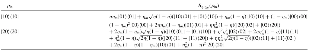
In this Appendix, we find input-output relationships for the butterfly module in Fig. 6. We do this in the number-state representation only for the relevant input states in Eq.(5).
TableIVprovides the output state for the butterfly operation
Bη,ηm when there is exactly one or two photons at one of the
input ports. These are the only relevant terms in the input states in Eqs. (3) and (4). Using Table IV, we find Bη,ηm(ρ
(in)
l )⊗
Bη,ηm(ρ
(in)
r ), to be used in Eq.(5).
The last operation required in Eq. (5) is the symmetric butterfly operation B0.5,ηd. Table V lists the input-output
relationships for all relevant input terms in our system for the more general operationB0.5,ηx. Note that by choosingηx =ηs,
we can use the same relationships for the measurement modules used in entanglement swapping and QKD of Figs.2
and3, respectively. For the sake of brevity, in TableV, we have only included the terms that provide us with nonzero values after applying the measurement operation. More specifically, we have removed allasymmetricdensity matrix terms, such as |1001| or|0110|, for which the bra state is different from the ket state, from the output state.
APPENDIX B: DERIVATION OFPclickANDPerror
In this Appendix, we find the gain and the QBER for the QKD scheme of Fig.3. Let us assume that the memory pairs
AB andCDare already entangled via the no-repeater or the one-node repeater scheme described in Sec.III. In the case of SPS protocol, their state is, respectively, given by Eqs.(7)and
TABLE IV. The input-output relationship for theBη,ηm operator.|j kj k| = |jJ Jj| ⊗ |kKKk|, whereJ =L′ andK=R′ for input number states andJ =LandK=Rfor output number states in Fig.6.
ρin Bη,ηm(ρin)
|1010| ηηm|0101| +ηm√η(1−η)(|1001| + |0110|)+ηm(1−η)|1010| +(1−ηm)|0000| (1−ηm)2|0000| +2ηηm(1−ηm)|0101| +ηηm2(1−η)(|2002| + |0220|)
|2020| +2ηm(1−ηm)√η(1−η)(|1001| + |0110|)+η2η2m|0202| +2ηη2m(1−η)|1111|
+η2
m(1−η)
√
2η(1−η)(|2011| + |1120|)+ηη2
m
√
2η(1−η)(|0211| + |1102|)
+2ηm(1−η)(1−ηm)|1001| +η2m(1−η)2|2020|
is then given byρABCD=B0.5,ηs(B0.5,ηs(ρAB⊗ρCD)),where
one of theB operators is applied to modesAandC and the other one to modesBandD.Using TableV, we can calculate the exact form ofρABCD, as we have done in this paper.
The most general measurement on the modes entering the photodetectors of Fig. 3, namely, A, B, C, andD, can be written in terms of the measurement operators
Mabcd = |aAAa| ⊗ |bBBb| ⊗ |cCCc| ⊗ |dDDd|
(B1) for PNRDs, where a, b, c, d=0,1 and |kK represents a
Fock state for the optical mode K=A, B, C, D. In the
case of NRPDs, we only need to replace |1KK1| with
(IK− |0KK0|), where IK is the identity operator for
modeK.
Similarly, we can define the corresponding probabilities to the above measurement operators as follows:
Pabcd =T r(ρABCDMabcd). (B2)
The explicit forms forPclickandPerrorare then given by
Pclick=PC+PE (B3)
TABLE V. The input-output relationship for a symmetric butterfly module. The notation used is similar to that of TableIV.
ρin B0.5,ηx(ρin)
|1010| ηx
2(|1010| + |0101|)+(1−ηx)|0000|
|0101| ηx
2(|1010| + |0101|)+(1−ηx)|0000|
|1111| ηx(1−ηx)(|1010| + |0101|)+(1−ηx)2|0000| + η2
x
2(|2020| + |0202|) |2020| ηx(1−ηx)(|1010| + |0101|)+(1−ηx)2|0000| +
ηx2
2|1111| +
ηx2
4(|2020| + |0202|) |0202| ηx(1−ηx)(|1010| + |0101|)+(1−ηx)2|0000| +η
2
2|1111| +
η2 x
4(|2020| + |0202|)
|2121| 3
2ηx(1−ηx)2(|1010| + |0101|)+(1−ηx)3|0000| + η2x
2(1−ηx)|1111|
+54η 2
x(1−ηx)(|2020| + |0202|)+38η 3
x(|3030| + |0303|)+
1 8η
3
x(|2121| + |1212|)
|2121| 32ηx(1−ηx)2(|1010| + |0101|)+(1−ηx)3|0000| + η2
x
2(1−ηx)|1111|
+54η 2
x(1−ηx)(|2020| + |0202|)+38η 3
x(|3030| + |0303|)+
1 8η
3
x(|2121| + |1212|)
|1001| 1
2ηx(|1010| − |0101|)
|0110| 1
2ηx(|1010| − |0101|)
|1120| √2
2 ηx(1−ηx)(|1010| − |0101|)+ 1 2√2η
2
x(|2020| − |0202|)
|1102| √2
2 ηx(1−ηx)(|1010| − |0101|)+2√12η2x(|2020| − |0202|)
|2011| √22ηx(1−ηx)(|1010| − |0101|)+2√12η2x(|2020| − |0202|)
|0211| √2
2 ηx(1−ηx)(|1010| − |0101|)+ 1 2√2η
2
x(|2020| − |0202|)
|2121| ηx(1−ηx)2(|1010| − |0101|)+η2x(1−ηx)(|2020| − |0202|)
+38η 3
x(|3030| − |0303|)+
1 8η
3
x(|1212| − |2121|)
|1212| ηx(1−ηx)2(|1010| − |0101|)+η2x(1−ηx)(|2020| − |0202|)
+3 8η
3
x(|3030| − |0303|)+
1 8η
3
x(|1212| − |2121|)
(1−ηx)4|0000| +2ηx(1−ηx)3(|1010| + |0101|)+η2x(1−ηx)2|1111|
|2222| +3
2η 3
x(1−ηx)(|3030| + |0303|)+12η 3
x(1−ηx)(|2121| + |1212|)
5 2η
2
x(1−ηx)2(|2020| + |0202|)+38η 4
x(|4040| + |0404|)+
1 4η
4
[image:11.608.51.557.382.757.2]and
Perror=edPC+(1−ed)PE, (B4)
whereedis the dephasing (misalignment) error,
PC =
⎧
⎪ ⎪ ⎪ ⎪ ⎪ ⎨
⎪ ⎪ ⎪ ⎪ ⎪ ⎩
(1−dc)2
P1100+P0011+dc(P1000+P0100+P0010+P0001)+2dc2P0000
,PNRD
d2 c
2 −dc+1
(P1100+P0011)+dc(1−d2c)(P1001+P0110)
+dc
2(2−dc)(P1000+P0100+P0010+P0001)+
d2 c
2(2−dc) 2P
0000
+12(P1110+P1101+P0111+P1011)+
dc
2(2−dc)(P1010+P0101)+ 1
2P1111,NRPD
(B5)
is the probability that Alice and Bob assign identical bits to their raw keys if there is no misalignment, and
PE=
⎧
⎪ ⎪ ⎪ ⎪ ⎪ ⎨
⎪ ⎪ ⎪ ⎪ ⎪ ⎩
(1−dc)2
P1001+P0110+dc(P1000+P0100+P0010+P0001)+2dc2P0000
,PNRD
d2 c
2 −dc+1
(P1001+P0110)+d2c(2−dc)(P1000+P0100+P0010+P0001)
+dc2
2(2−dc) 2P
0000+12(P1110+P1101+P0111+P1011)
+dc
2(2−dc)(P1100+P1010+P0011+P0101)+ 1
2P1111,NRPD
(B6)
is the probability that they make an erroneous bit assignment in the absence of misalignment.
[1] S. Wang, W. Chen, J.-F. Guo, Z.-Q. Yin, H.-W. Li, Z. Zhou, G.-C. Guo, and Z.-F. Han,Opt. Lett.37, 1008 (2012).
[2] M. Sasakiet al.,Opt. Exp.19, 10387 (2011).
[3] I. Choi, R. J. Young, and P. D. Townsend,New J. Phys. 13, 063039 (2011).
[4] M. Razavi,IEEE Trans. Commun.60, 3071 (2012).
[5] C. H. Bennett and G. Brassard, in Proceedings of the IEEE International Conference on Computers, Systems and Signal Processing, Bangalore(IEEE, New York, 1984), pp. 175–179. [6] H.-K. Lo, X. Ma, and K. Chen,Phys. Rev. Lett.94, 230504
(2005).
[7] A. K. Ekert,Phys. Rev. Lett.67, 661 (1991).
[8] C. H. Bennett, G. Brassard, and N. D. Mermin,Phys. Rev. Lett.
68, 557 (1992).
[9] H.-J. Briegel, W. D¨ur, J. I. Cirac, and P. Zoller,Phys. Rev. Lett.
81, 5932 (1998).
[10] L. M. Duan, M. D. Lukin, J. I. Cirac, and P. Zoller, Nature (London)414, 413 (2001).
[11] J. Amirloo, A. H. Majedi, and M. Razavi,Phys. Rev. A 82, 032304 (2010).
[12] S. Abruzzo, S. Bratzik, N. K. Bernardes, H. Kampermann, P. van Loock, and D. Bruß,Phys. Rev. A87, 052315 (2013).
[13] L. Jiang, J. M. Taylor, and M. D. Lukin,Phys. Rev. A76, 012301 (2007).
[14] Z.-B. Chen, B. Zhao, Y.-A. Chen, J. Schmiedmayer, and J.-W. Pan,Phys. Rev. A76, 022329 (2007).
[15] C. Simon, H. de Riedmatten, M. Afzelius, N. Sangouard, H. Zbinden, and N. Gisin,Phys. Rev. Lett.98, 190503 (2007).
[16] N. Sangouard, C. Simon, B. Zhao, Y.-A. Chen, H. de Riedmatten, J.-W. Pan, and N. Gisin,Phys. Rev. A77, 062301 (2008).
[17] N. Sangouard, C. Simon, J. Min´aˇr, H. Zbinden, H. de Riedmatten, and N. Gisin,Phys. Rev. A76, 050301 (2007).
[18] N. Sangouard, C. Simon, H. de Riedmatten, and N. Gisin,Rev. Mod. Phys.83, 33 (2011).
[19] E. Bocquillon, C. Couteau, M. Razavi, R. Laflamme, and G. Weihs,Phys. Rev. A79, 035801 (2009).
[20] M. Razavi, I. S¨ollner, E. Bocquillon, C. Couteau, R. Laflamme, and G. Weihs,J. Phys. B42, 114013 (2009).
[21] J. Claudon, J. Bleuse, N. S. Malik, M. Bazin, P. Jaffrennou, N. Gregersen, C. Sauvan, P. Lalanne, and J.-M. Ger´ard,Nat. Photon.4, 174 (2010).
[22] H.-K. Lo, M. Curty, and B. Qi,Phys. Rev. Lett.108, 130503 (2012).
[23] A. Rubenok, J. Slater, P. Chan, I. Lucio-Martinez, and W. Tittel,
arXiv:1304.2463.
[24] C. H. Bennett,Phys. Rev. Lett.68, 3121 (1992).
[25] H.-K. Lo, M. Curty, and B. Qi,Phys. Rev. Lett.108, 130503 (2012).
[26] X. Ma and M. Razavi, Phys. Rev. A 86, 062319 (2012).
[27] X. Ma, Chi-Hang Fred Fung, and M. Razavi,Phys. Rev. A86, 052305 (2012).
[28] M. Razavi, N. Lo Piparo, C. Panayi, and D. E. Bruschi,Iran Workshop on Communication and Information Theory (IWCIT), Tehran, Iran, 2013(IEEE, Piscataway, NJ, 2013), invited paper. [29] M. Razavi, M. Piani, and N. L¨utkenhaus, Phys. Rev. A 80,
032301 (2009).
[30] M. Razavi, K. Thompson, H. Farmanbar, M. Piani, and N. L¨utkenhaus, in Quantum Communications Realized II, edited by Y. Arakawa, M. Sasaki, and H. Sotobayashi (SPIE, Bellingham, WA, 2009), Vol. 7236, p. 723603.
[31] P. W. Shor and J. Preskill, Phys. Rev. Lett. 85, 441 (2000).
[32] M. Afzelius, C. Simon, H. de Riedmatten, and N. Gisin,Phys. Rev. A79, 052329 (2009).
[33] P. L. Knight and A. Miller, inMeasuring the Quantum State of Light, 1st ed. (Cambridge University Press, Cambridge, 1997), Vol. 1.
[34] M. Razavi and J. H. Shapiro, Phys. Rev. A 73, 042303 (2006).