Automatically Improving Constraint Models in Savile Row through Associative-Commutative Common Subexpression Elimination

This is a repository copy of

Automatically Improving Constraint Models in Savile Row

through Associative-Commutative Common Subexpression Elimination

.

White Rose Research Online URL for this paper:

http://eprints.whiterose.ac.uk/144177/

Version: Accepted Version

Proceedings Paper:

Nightingale, Peter orcid.org/0000-0002-5052-8634, Akgun, Ozgur, Gent, Ian Philip et al. (2

more authors) (2014) Automatically Improving Constraint Models in Savile Row through

Associative-Commutative Common Subexpression Elimination. In: Principles and Practice

of Constraint Programming. Lecture Notes in Computer Science . SPRINGER , Cham , pp.

590-605.

https://doi.org/10.1007/978-3-319-10428-7_43

[email protected] https://eprints.whiterose.ac.uk/

Reuse

Items deposited in White Rose Research Online are protected by copyright, with all rights reserved unless indicated otherwise. They may be downloaded and/or printed for private study, or other acts as permitted by national copyright laws. The publisher or other rights holders may allow further reproduction and re-use of the full text version. This is indicated by the licence information on the White Rose Research Online record for the item.

Takedown

If you consider content in White Rose Research Online to be in breach of UK law, please notify us by

Automatically Improving Constraint Models in Savile

Row through Associative-Commutative Common

Subexpression Elimination

Peter Nightingale, ¨Ozg¨ur Akg¨un, Ian P. Gent, Christopher Jefferson, and Ian Miguel

School of Computer Science, University of St Andrews, St Andrews, Fife KY16 9SX, UK

{pwn1, ozgur.akgun, ian.gent, caj21, ijm}@st-andrews.ac.uk

Abstract. When solving a problem using constraint programming, constraint modelling is widely acknowledged as an important and difficult task. Even a constraint modelling expert may explore many models and spend considerable time modelling a single problem. Therefore any automated assistance in the area of constraint modelling is valuable. Common sub-expression elimination (CSE) is a type of constraint reformulation that has proved to be useful on a range of problems. In this paper we demonstrate the value of an extension of CSE called

Associative-Commutative CSE (AC-CSE). This technique exploits the

proper-ties of associativity and commutativity of binary operators, for example in sum constraints. We present a new algorithm, X-CSE, that is able to choose from a larger palette of common subexpressions than previous approaches. We demon-strate substantial gains in performance using X-CSE. For example on BIBD we observed speed increases of more than 20 times compared to a standard model and that using X-CSE outperforms a sophisticated model from the literature. For Killer Sudoku we found that X-CSE can render some apparently difficult in-stances almost trivial to solve, and we observe speed increases up to 350 times. For BIBD and Killer Sudoku the common subexpressions are not present in the initial model: an important part of our methodology is reformulations at the pre-processing stage, to create the common subexpressions for X-CSE to exploit. In summary we show that X-CSE, combined with preprocessing and other reformu-lations, is a powerful technique for automated modelling of problems containing associative and commutative constraints.

1

Introduction

When solving a problem using constraint programming, constraint modelling is widely acknowledged as both important and difficult [13]. A problem may have many mod-els, and it is difficult to know which will be solved most efficiently by a given con-straint solver. Even a concon-straint modelling expert may explore many models and spend considerable time modelling a single problem. Therefore, any automated assistance in constraint modelling is valuable.

performed separately for each problem instance, hence any computationally expensive reformulation must pay for itself by saving time during solving.

Common sub-expression elimination (CSE) is a type of constraint reformulation that has proved to be useful on a range of problems [16, 15]. Herein we investigate an extension of CSE,Associative-CommutativeCSE (AC-CSE), which exploits the proper-ties of associativity and commutativity of binary operators (e.g.+and×). Expressions containing these operators can be rearranged to reveal common subexpressions. As an example, take the following two constraints over four variables:

w+x+y+z= 6, z+y+w= 5

Conventional constraint propagation will not reveal the fact thatx= 1. AC-CSE could extractw+y+zand replace it with an auxiliary variableato give the following three constraints. Performing constraint propagation on this set will assignxto1.

x+a= 6, a= 5, a=w+y+z

An Associative-Commutative Common Subexpression (AC-CS) of a set of associative and commutative (AC) expressions (e.g. sums) is a set of at least two terms that all appear in each one of the AC expressions (sums). In the example above, the set of three terms{w, y, z}appears in both the original sum constraints, hence{w, y, z}is an AC-CS of the two sum constraints.

A simple normalisation step, such as sorting the terms in the AC expressions, fol-lowed by examining contiguous subsequences of terms within AC expressions, can reveal some but not all of the available AC-CSs. More is necessary to find AC-CSs in general. Consider the example above, with an alphabetical ordering of the terms

w+x+y+zandw+y+z. The largest contiguous subsequence of both isy+z, so this approach would miss the maximal AC-CSw+y+z.

In this paper we introduce and describe in detail a new algorithm, X-CSE, to per-form AC-CSE in constraint problems. We show that X-CSE is able to find common subexpressions (CSs) automatically in a variety of problems, and that using these subex-pressions can greatly reduce search and improve solving time. A particular advantage of X-CSE is that it is able to find and exploit small CSs that occur in many constraints, as well as larger ones that occur in few constraints. This is made possible by finding CSs that contain auxiliary variables introduced at an earlier step of the algorithm. We can thus exploit the occurrence of many small CSs without losing the advantages of finding larger ones. We illustrate this with an example below in Sections 2.3 and 3.3. The reuse of auxiliary variables created by AC-CSE in subsequent common subexpressions is an important advantage of X-CSE.

We evaluate the new algorithm on four problem classes: BIBD, the SONET prob-lem, Killer Sudoku and Molnar’s Problem. When applying X-CSE we demonstrate sub-stantial gains in performance. On BIBD we observed speed increases of more than 20 times compared to a standard model. We found that X-CSE outperforms a sophisticated model from the literature with manually derived implied constraints [7]. On the SONET problem we observed speed increases of 5 times on some instances. For Killer Sudoku we found that applying X-CSE can render some apparently difficult instances almost trivial to solve, and we saw more than 300 times speed increases in some cases. Mol-nar’s Problem exhibits more modest gains peaking at 5 times faster for the most difficult instance.

2

Related Work

The context of our work is reformulation of constraint modelling languages such as OPL [19], MiniZinc [18] and ESSENCE′ [16]. These languages have a collection of global constraints, arithmetic and logical operators that act on finite-domain or real interval decision variables. In this paper we consider finite-domain decision variables.

Such languages are not directly accepted by constraint solvers but must be tailored into a form suitable for a constraint solver. During tailoring the model can be

refor-mulated to improve the efficiency of the constraint solver. There are many ways of

producing better constraint models, some requiring manual interaction [2], and others that are automated [8]. For example these tools can discover global constraints or auto-matically detect and remove symmetries [11]. These improvements often complement each other, for example Frisch, Jefferson, and Miguel [7] show how breaking symme-tries can lead to effective implied constraints for BIBDs among other problems. In this paper we show how to automatically generate a superior model for the BIBD problem.

2.1 Flattening and CSE

Flattening is the process of taking a nested expression and reducing the degree of nest-ing by replacnest-ing a subexpression with a new variable. For example given the product

X×(Y +Z)and a target solver that does not allow sums inside products, the flatten-ing process will add a new variableaux, replace the product with the new expression

X×auxand add a new constraintaux=Y+Z. We say thatX×(Y+Z)isflattened

toX×auxand thatY +Zisextracted.

Common sub-expression elimination (CSE) was first applied in the context of finite-domain constraint languages by Andrea Rendl [16, 15]. In its simplest form, CSE takes two or more syntactically identical sub-expressions that must be flattened, and flattens them all using the same auxiliary variable. This reduces both the number of constraints and auxiliary variables. Importantly, CSE can reduce the search space dramatically [16, 15] by linking different constraints together thus strengthening constraint propagation.

2.2 Normalisation and Active CSE

normali-sation, where prior to CSE the expression tree is converted to a normal form (pri-marily by ordering the arguments of commutative operators and evaluating any con-stant expressions). This converts some semantically equivalent expressions (such as

C=B+A+ 1−1andA+B=C) to syntactically identical expressions. The second

isActive CSE, where two expressionsAandB may be matched if they are identical

after some transformation (for example by applying one of De Morgan’s laws). For example, Active CSE can matchA < BwithA≥Bby a simple negation.

The algorithm introduced by Rendl [15] and used by Stuckey and Tack [18] per-forms CSE during flattening. The algorithm maintains a hash table keyed by the ex-pressions that have been extracted so far, and containing the new auxiliary variable for each. When extracting an expressionE, the algorithm looks up E in the hash table, and (if present) uses the auxiliary variable in the hash table rather than creating a new auxiliary. This algorithm has the advantage that is easily extended to active CSE. When looking upE in the hash table, active CSE also looks up each transformation ofE. However it is not clear how this algorithm could be extended to AC-CSE. The common subexpressions extracted by AC-CSE would not normally be extracted by flattening.

2.3 Associative-Commutative CSE

Araya, Neveu and Trombettoni [1] exploited common subexpressions among+and× expressions. Their work is in the context of numerical CSP solved by algorithms such as HC4, but the reformulation is equally applicable to finite-domain CSP. They proposed two algorithms named I-CSE and I-CSE-NC. Both algorithms apply a form of AC-CSE prior to flattening as a separate operation.

The first pass of both algorithms is to transform the abstract syntax tree (AST) into a directed acyclic graph where identical subexpressions are represented once. The second step is to intersect each pair of sums and pair of products to create a set of candidate AC-CSs. As we will see in Section 3.3 other AC-CSs (generated by the intersection of three or more sums) can also be useful, but I-CSE and I-CSE-NC will never generate them. Later passes extract the AC-CSs from the original expressions.

Araya et al. defined two AC-CSsf1andf2to bein conflictiff1∩f26=∅,f1*f2 andf2 *f1. Two AC-CSs in conflict cannot both be extracted from the same expres-sion. When a set of AC-CSs in conflict are subsets of the same original expressions, then I-CSE copiessa sufficient number of times to extract each of the AC-CSs from at least one copy. I-CSE-NC (for No Conflicts) does not copys, it simply extracts a single maximal subset of the candidate AC-CSs froms. Consider the following example:

v+w+x+y= 0, v+w+x+z= 0

v+w+y+z= 0

In this example I-CSE(-NC) would generate three AC-CSs:v +w+x, v+w+y

andv+w+z. I-CSE would duplicate each of the original constraints resulting in six constraints and three further constraints to define the auxiliary variables.

I-CSE-NC can extract only one AC-CS. Suppose it extractsv+w+x, then at this pointv+w+yandv+w+zcease to be AC-CSs:

aux=v+w+x

I-CSE-NC can only extract CSEs from the original expressions, so fails to exploit the AC-CSv+w. Even on this small example I-CSE has increased the size of the model substantially. I-CSE-NC has not, but it has missed a potentially useful AC-CS and has not linkedv+w+y+zto the other two sums.

I-CSE and I-CSE-NC are both compared to our algorithm in the experiments below. We implement the algorithms exactly as described in Section 4 of Araya et al. [1]. Both I-CSE and I-CSE-NC only extract AC-CSs from the original expressions, they do not extract AC-CSs from other AC-CSs.

3

The X-CSE Algorithm

The X-CSE algorithm is implemented in Savile Row 1.6 [12]. Savile Row reads the ESSENCE′ language and transforms it in many passes to an output for a constraint solver. X-CSE simply becomes another pass. In this paper we consider the associa-tive and commutaassocia-tive (AC) operators\/(or),/\(and),+,*. These are represented as a single AST node withnchildren in Savile Row 1.6. There are other AC operators in the language, notablyminandmax, and!=between boolean expressions (exclusive or). We leave these for future work.

Prior to running X-CSE the AST is normalised by sorting the children of all com-mutative operators. For any AC operator⋄, the goal of X-CSE is to find common sets containing two or more expressions that are contained in more than one⋄expression. The X-CSE algorithm uses a hash tablemapfrompairsof expressions{a, b}to a list of the⋄expressions that contain bothaandb. Algorithm 2 (populateMap) takes a ref-erence to an AST node and explores the tree, populatingmapfor each⋄expression.

Algorithm 1 (X-CSE) takes a reference to the AST representing all constraints, a reference to the global symbol table, and the AC operator⋄. After initialising data structures it calls populateMap with the entire AST. Following that it enters the main loop on line 4. On line 5 one pair is selected frommapaccording to a heuristic. If the pair occurs in more than one⋄expression then there must exist an AC-CS including that pair. Lines 10-20 find an AC-CS and extract it from all the relevant expressions. The algorithm includes as many ⋄expressions as possible to maximise the effect of extracting the AC-CS. Line 10 intersects all⋄expressions containing the pair. A new⋄ expression for the AC-CS is constructed, and an auxiliary variable is created. On line 14 a constraint is created to define the auxiliary variable. Each ⋄ expression containing the AC-CS is replaced. At this point, lines 19 and 20 updatemap to include all the newly created expressions, allowing X-CSE to extract further AC-CSs from the new expressions. Some references to removed⋄expressions will remain inmap; these will be filtered out on line 8.

3.1 Heuristics

Algorithm 1X-CSE(AST_,ST_,⋄)

Require: AST: Abstract syntax tree representing the model Require: ST_{: Symbol table containing decision variables}

Require: ⋄: The associative and commutative operator

1: newcons←empty list{Collect new constraints}

2: map←empty hash table mapping pairs of expressions to lists 3: populateMap(AST,map,⋄)

4: whilemapnot emptydo

5: pairexp←heuristic(map)

6: ls←map(pairexp){lsis a list of⋄AST nodes}

7: deletemap(pairexp)

8: ls←filter(isAttached,ls){Remove⋄AST nodes no longer contained inAST_ornewcons}

9: iflength(ls)>1then

10: commonset←ls[1]∩ls[2]∩ · · · ∩ls[length(ls)]

11: e←fold(⋄,commonset) 12: bnds←bounds(e)

13: aux←ST_{.newAuxVar(bnds)}

14: newc←(e=aux){New constraint definingaux}

15: newcons.append(newc)

16: for alla∈ls_do

17: newe←fold(⋄,(a\commonset_{)∪ {}aux_}) 18: ReplaceawithnewewithinAST_ornewcons

19: populateMap(newe,map,⋄) 20: populateMap(newc,map,⋄) 21: AST←AST∧fold(∧,newcons)

largest AC-CS and smallest AC-CS. In some cases there exists a pair such that its cor-responding AC-CS can be extracted without preventing any other AC-CS. We call these

non-blocking pairsand it may be helpful to process them first. We created four more

heuristics that select non-blocking pairs first, then fall back to one of the four basic heuristics. We found no clear winner among the eight heuristics. We use the ‘most oc-currences’ heuristic throughout the rest of this paper because it is cheap to compute and often performs well.

Algorithm 2populateMap(A,map,⋄) Require: A: Reference to an abstract syntax tree

Require: map: Hash table mapping pairs of expressions to lists Require: ⋄: The associative and commutative operator

3.2 Complexity Analysis

In this analysis we will usenfor the number of⋄expressions,kfor the length of the longest⋄expression,das the depth of the deepest⋄expression in the AST, andSas the number of nodes in the AST.

Central to the complexity analysis of X-CSE is the observation that at mostk−1

AC-CSs may be extracted from one⋄by X-CSE. Recall (from Section 2.3) that two AC-CSs in conflict cannot both be extracted from the same expression. A pair of AC-AC-CSs may overlap only if one is a subset of the other. Consider an AC-CSfin an expressione. There can be no other AC-CSs involvingfineexcept possibly somef′_{wheref (f}′_.

The smallest AC-CS is size two, and extracting this replaces a size two term with a size one term (i.e. the replacement auxiliary variable). If the original expression is sizek, we thus find one AC-CS and now have a sizek−1expression. Iterating shows that at mostk−1AC-CSs may be extracted from one⋄expression by X-CSE. This gives us a global limit ofO(nk)AC-CS extractions.

To populate map, populateMap traverses the AST with S nodes, and for each⋄ expressioneit inserts a reference toeinO(k2_{)lists withinmap. Assuming hash table} operations areO(1), populateMap takesO(S+nk2_)time.1

X-CSE then enters a loop that continues untilmapis empty. Each iteration of the loop is as follows. We assume the heuristic takesO(1)time.2For the given pair, its list

lshas at mostnelements. Note that if the pair occurs more than once in an expression it might be entered intolsmultiple times: to keep the list at sizen, when inserting an expressioneintolswe can check the last element ofls: if it is equal toe, we do not insertefor a second time. The listlsis filtered inO(nd)time. If the list has length two or greater, then we extract an AC-CS. For the following we assume that an AC expres-sion is represented by a set data structure withO(1)lookup, insertion and removal.3

Creatingcommonseton line 10 takesO(nk)time. Computing the bounds and creating the auxiliary variable and the new constraint can be done inO(k)time. The algorithm then replacescommonsetin eachlsexpression inO(nk)time. Re-populatingmap(on lines 19 and 20) takesO(S+nk2_{)because the updated AC expressions can contain the} entire AST. Therefore the entire cost of extracting one AC-CS isO(S+nk2_{+nd), and} the total cost of X-CSE isO(nkS+n2_k3_+n2_kd).

While the complexity may seem high, the algorithm scales with the number of AC-CSs it is able to exploit, therefore it is relatively quick when there are few or no AC-AC-CSs, and it takes more time when there is greater potential benefit.

3.3 Comparison with I-CSE(-NC)

X-CSE differs from the existing algorithms I-CSE(-NC) in that it can extract AC-CSs that are intersections of more than two expressions, and AC-CSs containing auxiliary

1_{This is correct if all expressions to be hashed are sizeO(1)and computing the hash code is}

linear. If either assumption is invalid then an additional factorhis necessary, representing the time to hash an expression.

2

As an example of anO(1)heuristic we could maintain a doubly linked list of keys inmapand have the heuristic simply remove and return the first element of the list.

variables (from earlier steps). Thus it has a larger palette of AC-CSs to choose from. In the example from Section 2.3, X-CSE would first extractv+wfrom all three sums as follows.

a=v+w, a+x+y= 0, a+x+z= 0, a+y+z= 0

Second, X-CSE would extract any one ofa+x,a+yora+z, as follows. This second step is not possible in I-CSE(-NC).

a=v+w, b=a+x, b+y= 0, b+z= 0, a+y+z= 0

This result is clearly better than I-CSE-NC (Section 2.3) that extracted onlyv+w+x

and thus did not connect the third constraint to the other two. I-CSE produced nine constraints on this example. It is possible that the more compact model produced by X-CSE is better. We investigate this further in Section 5.5.

4

Preprocessing and Reformulation

The number and quality of CSs found can be improved by using MINIONto preprocess an initial version of the model then feeding it back into Savile Row for CSE. Our method is as follows. First Savile Row translates the instance to MINION(with or without X-CSE). Then MINIONis called to filter domains with SACBounds (no search), which is a variant of SAC [3]. SACBounds applies the SAC test to prune the upper and lower bound of each variable to exhaustion. Savile Row re-starts the translation process with the filtered domains and translates the instance to MINIONagain (with or without X-CSE). Re-starting translation allows Savile Row to simplify the constraints following domain filtering. For example, on the BIBD problem below, some variables are assigned by SACBounds and this allows constant folding (e.g.· · ·+a×x+b×y+· · · where SACBounds assignsa= 1andb= 0becomes· · ·+x+· · ·).

A further step to promote the identification of AC-CSs is in reformulating a model to add implied constraints consisting of AC expressions. Savile Row creates implied sum constraints from all-different and global cardinality constraints. This is done by finding assignments to the all-different (GCC) with the smallest and largest sums (lbandub

resp.), then adding eitherP_≥lb

andP_≤ub

(whenlb6=ub) orP

=lb=ubwhere P

is the sum of the variables in scope of the original constraint (except cardinality variables in GCC). For example, givenallDiff(x, y, z)where all variables have domain {1. . .4}, we add constraintsx+y+z≥1 + 2 + 3andx+y+z≤2 + 3 + 4.

5

Case Studies

by Savile Row (which includes the first preprocessing call to MINION) and total time reported by MINION1.6.1 64-bit to search for a solution. MINIONis given a time limit of 600s to solve the final model. Savile Row is executed in the Java 1.7.0 55 JIT. Each reported timing is a mean of 5 runs. Experiments were performed on a 32-core AMD Opteron 6272 at 2.1 GHz. All model and parameter files are available athttp://pn. host.cs.st-andrews.ac.uk/cp-2013-ac-cse-experiments.tgz.

5.1 Case study 1: BIBD

We use Puget’s model of the Balanced Incomplete Block Design (BIBD) problem, with

Lex2symmetry breaking constraints [14]. BIBD is parameterised by(v, k, λ)and has

r = λ(v−1)

k₋1 andb =

λv(v₋1)

k(k₋1). The model has avbybmatrixmof boolean variables. Each of thevrows sums tor(row constraints), and each of thebcolumns sums tok

(column constraints). The scalar product of each pair of rows has valueλ:

∀i1, i2∈ {1. . . v}. i1< i2→( b X

j=1

m[i1, j]∗m[i2, j]) =λ

This model initially has no common subexpressions (identical or AC). As described above the domains are filtered by applying SACBounds. This assigns some of the vari-ables (the entire first two rows and first column, plus some other entries). When trans-lating again with the domains filtered by SACBounds, the scalar product constraints are simplified causing AC-CSs to appear among scalar product constraints, and between scalar product and row sum constraints.

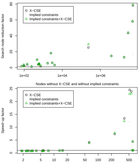
We evaluated X-CSE on the 24 instances in Figure 1 of Puget ([14]). MINIONtimes out for 4 instances without X-CSE. For the remaining 20 instances, X-CSE always decreases the node count. Figure 1 plots the reduction factor for the 20 instances. Harder instances tend to show a greater reduction in node count. For the hardest instance solved within the time limit, the node count is reduced by 78 times.

Figure 1 plots speed-up of total time with X-CSE. For the easiest instances, the re-duction in node count does not cause a measurable difference in MINION’s run time. The slow down in total time is caused by the up-front cost of X-CSE. On the harder instances, MINIONsearch takes up most of the total time and X-CSE speeds up search substantially by reducing the number of search nodes. Figure 1 (lower) peaks with in-stance(10,3,6), which has a 58-fold reduction in nodes and speed up of 24.5 times. X-CSE typically increases the number of constraints and auxiliary variables, reducing the node rate of MINION. Finally,(10,3,8)times out without X-CSE, and takes 138.6 s with X-CSE. Hence it appears on the far right of Figure 1 with a speed up of 4.39.

1e+02 1e+04 1e+06

0

20

40

60

80

Nodes without X−CSE and without implied constraints

Search node reduction f

actor

● ●

●

●

● ●

● ● ●

●

● ●

●

● ● ● ●

● ●

● ●

X−CSE Implied constraints Implied constraints+X−CSE

2 5 10 20 50 100 200 500

0

5

10

15

20

25

Total time without X−CSE and without implied constraints (s)

Speed−up f

actor

● ●

●

●

●

● ●

● ● ●

● ● ● ● ●●●

● ● ● ●

●

●

● ●

X−CSE Implied constraints Implied constraints+X−CSE

Fig. 1.(Top) BIBD search nodes of instances that do not time out. (Bottom) BIBD total time.

from the row constraint for rowi and scalar product with either row 1 or 2 using an approach resembling manual AC-CSE.

The automated approach improves on Frisch et al. in two ways. First SACBounds is able to assign not just the first two rows and first column but also parts of other rows and columns. For example, on the instance(v = 22, k = 7, λ = 2)parts of the third and fourth rows and the first eight entries of the second column are assigned. Second, X-CSE is able to link multiple scalar product constraints and a row constraint, whereas the implied constraints are each derived from a single scalar product constraint and a row constraint.

0.2 0.5 2.0 5.0 20.0 100.0 500.0 1 2 3 4 5 6

Total time without X−CSE (s)

Speed up f

actor with X−CSE

● ● ● ● ● ● ● ● ● SONET Molnar's ● ● ● ● ● ● ● ● ● ● ● ● ●● ● ● ● ● ● ● ● ● ● ● ● ● ● ● ● ● ● ● ● ● ● ● ● ● ● ● ● ● ● ● ● ● ● ● ● ● ● ● ● ● ● ● ●●●● ● ● ● ● ● ● ● ● ● ● ● ● ● ● ● ● ● ● ● ● ● ● ● ● ● ● ● ●● ● ● ●●●●●●● ● ●

2 5 10 20 50 100 200 500

0

50

150

250

350

Total time without X−CSE (s)

Speed up f

actor with X−CSE

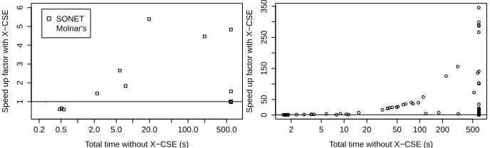
Fig. 2.(Left) Results for SONET and Molnar’s Problem total time. (Right) Results for Killer Sudoku total time.

5.2 Case study 2: The SONET problem

The SONET problem [17] is a network design problem where each node is connected to a set ofrings(fibre-optic connections). The simplified SONET problem (Section 3 of [17]) where each ring has unlimited capacity has the following parameters: the number of nodesn, the upper limit on the number of ringsm, the maximum number of nodes per ringr, and a set of pairs that must be connected. For each of these pairs there must exist a ring connected to both nodes. The number of node-ring connections is minimised.

The problem is modelled as follows. We have a boolean matrixringsindexed by

[1. . . m,1. . . n].rings[a, b]indicates whether ringais connected to nodeb. For each ringawe have the sum constraintPn_b=1rings[a, b]≤r. The connectedness constraint between two nodesb1andb2is expressed as a disjunction (refined by Savile Row to a watched-or [9]) of sums:

∃i∈ {1. . . m}.(rings[ai, b1] +rings[ai, b2]≥2)

The minimisation function is simply the sum ofrings. Rings are indistinguishable so we use lexicographic ordering constraints to order the rows ofringsin non-decreasing order. The static variable ordering we use is the reading order ofringsand value order is 0 then 1. This model is very simple and does not include implied or dominance constraints [17]. The problem constraints are already flat and only the minimisation sum needs to be flattened, thus only one auxiliary variable is created by Savile Row without X-CSE. There are AC-CSs between the connectedness constraints, the ring sum constraints and the minimisation sum.

We generated 24 instances withn ∈ {6. . .13},r ∈ {3,4,5}, andm = 10. The demand graph when n = 13 is Figure 1 of Smith [17]. For smaller n we take the subgraph with vertices{n+ 1. . .13}and edges adjacent to these vertices removed.

5.3 Case study 3: Killer Sudoku

We consider the Killer Sudoku problem. The standard Killer Sudoku has a9×9grid where each row and column are all-different, and the nine non-overlapping3×3 sub-squares are also all-different. Each slot in the grid is initially empty and takes a digit

1. . .9. Clues are sets of squares that sum to a given value (and are also all-different). We found that9×9Killer Sudoku instances were very easy. We generalised the puzzle to16×16with16 4×4subsquares, and each slot takes a number1. . .16. 100 in-stances were generated at random. Traditional Killer Sudoku puzzles have exactly one solution. The random16×16instances may be unsatisfiable and may have multiple solutions. For brevity we do not describe how these instances are generated. All models and instances are available on the web at the URL given in Section 5 above.

X-CSE alone does nothing because the sums in the clues are the only AC expres-sions and they do not overlap. However the sums overlap with all-different constraints. Each all-different constraint on a row, column or subsquare represents a permutation of {1. . .16} which sum to136. Savile Row automatically adds these implied sum con-straints as described in Section 4. X-CSE is able to find common subexpressions among rows, columns, sub-squares and clues.

Figure 2 plots the speed-up quotient for Killer Sudoku. Without X-CSE, 54 in-stances timed out. With X-CSE, 28 inin-stances timed out. As the inin-stances become more difficult the trend is towards greater speed-up by X-CSE. The plot peaks at 345 times faster. On this instance, without X-CSE Savile Row took 2.26 s and MINIONtimed out after exploring 2,774,028 nodes. With X-CSE, Savile Row took 1.62 s and MINION

took 0.13 s to explore 2 nodes.

5.4 Case study 4: Molnar’s Problem

Molnar’s problem [6] (CSPLib problem 035 [5]) is to find a square matrixM of inte-gers. The model has two parameters: the sizek(i.e.M has sizek×k) and the maximum absolute value of integers inM, namedd. The initial domain of each element ofM is {−d . . .−2} ∪ {0} ∪ {2. . . d}. The first constraint is that the determinant ofM is1

or−1(following the model of Frisch et al. [6]). For the second constraint we construct another matrixSwhere each entry ofSis the square of the corresponding entry ofM. The determinant ofSmust also be1or−1.

We used the Leibniz formula for determinants, and expresseda2_{asa×ato allow} more AC-CSs of products. Whenk = 3we have the following two matrices and two constraints. In addition we break symmetry onM by lexicographically ordering rows and columns.

M =

_{a b c} d e f g h i

, S=

_a2 _b2 _c2

d2 _e2_f2

g2_h2 _i2

|M|=aei−af h+bf g−bdi+cdh−ceg∈ {−1,1}

|S|=aaeeii−aaf f hh+bbf f gg−bbddii+ccddhh−cceegg∈ {−1,1}

particular AC-CS from the same product more than once on this problem. Consider

aei: extracting it once creates a new constraintaei=xand modifies the expressionaei

tox, and the expressionaaeeiitox×aei. Now X-CSE extractsaeia second time from the new constraint and one of the modified expressions, creating a second auxiliary variable (that will later be unified withx).

Figure 2 plots the speed-up quotient for Molnar’s Problem on the eight instances wherek ∈ {2,3} andd ∈ {2. . .5}. X-CSE appears to be more useful for the more difficult instances. None of the instances time out. The peak speed-up quotient is 5.5.

5.5 I-CSE and I-CSE-NC

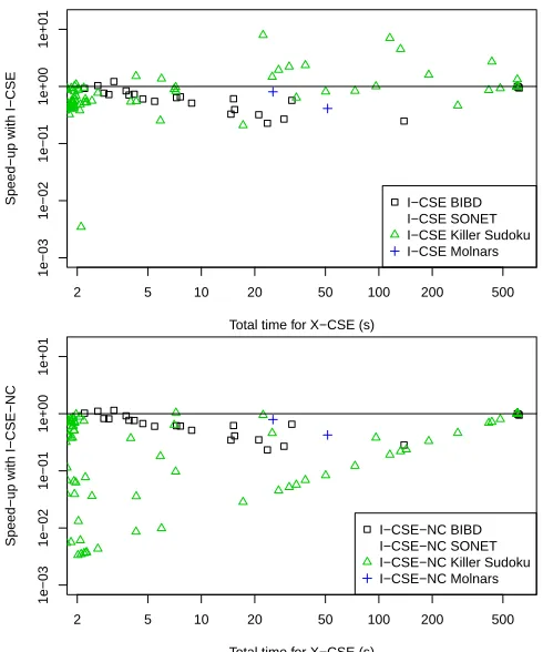
In this section we use all four problem classes to compare X-CSE to I-CSE and I-CSE-NC. Figure 3 plots the speed-up factor for I-CSE and I-CSE-NC compared to X-CSE. It is clear from the lower plot that I-CSE-NC performs much more poorly than X-CSE (since almost all points are belowy = 1). By comparing the two plots in Figure 3 it is clear that I-CSE outperforms I-CSE-NC on Killer Sudoku, I-CSE-NC is preferable for SONET, and that the two algorithms are very similar for BIBD (without implied constraints) and Molnar’s Problem.

X-CSE performs substantially better than I-CSE on BIBD and SONET, and slightly better on Molnar’s Problem. For BIBD, both timed out on 3 instances and each solved 21. X-CSE explored fewer search nodes on 16 of the 21 instances, and was much faster overall. The mean time for X-CSE (on the set of 21 instances) was 16.7 s compared to 52.1 s for I-CSE.

For SONET, X-CSE always explores more (or an equal number of) search nodes than I-CSE but total time is lower with X-CSE for all instances taking longer than 1 s. X-CSE was able to solve all instances that I-CSE could within the timeout, and one additional one. Of the 9 that both solved, X-CSE had a mean time of 20.3 s compared to I-CSE’s mean of 65.1 s. X-CSE and I-CSE-NC are able to solve the same set of 10 SONET instances. X-CSE had a mean time of 57.1 s while I-CSE-NC had a mean time of 59.7 s.

For Killer Sudoku, the picture is less clear. 70 instances are solved by both I-CSE and X-CSE. I-CSE solves one additional instance in 454 s, and X-CSE solves two additional instances in 2.1 s and 278 s. On the 70 instances solved by both, I-CSE took a mean time of 28.6 s, and X-CSE took a mean time of 35.2 s. I-CSE searches fewer nodes on 16 of these 70 instances and is more than 1.5 times faster than X-CSE on 10 instances. In short, neither X-CSE nor I-CSE is clearly better than the other on Killer Sudoku. The successes of I-CSE show that it can be worthwhile to extract conflicting AC-CSs.

5.6 Other Problems

2 5 10 20 50 100 200 500

1e−03

1e−02

1e−01

1e+00

1e+01

Total time for X−CSE (s)

Speed−up with I−CSE

● ●

● ●

● ●

●

● ● ● ● ● ● ● ● ● ● ● ● ●

●

I−CSE BIBD I−CSE SONET I−CSE Killer Sudoku I−CSE Molnars

2 5 10 20 50 100 200 500

1e−03

1e−02

1e−01

1e+00

1e+01

Total time for X−CSE (s)

Speed−up with I−CSE−NC

●

● ●

● ● ● ●●●●●●●●●●●●●●

●

I−CSE−NC BIBD I−CSE−NC SONET I−CSE−NC Killer Sudoku I−CSE−NC Molnars

Fig. 3.Comparison of X-CSE with I-CSE (top) and I-CSE-NC (bottom).

Figure 4 (left) plots the time taken by Savile Row (including running MINIONto enforce SACBounds). In some cases applying X-CSE speeds up Savile Row overall. Figure 4 (right) plots total time. Only two problems searched fewer nodes with X-CSE: Plotting (2% reduction) and waterBucket (21% reduction) and for both these problems the search time saved is outweighed by additional time required in Savile Row. For those problems that are sped up overall, there are two reasons: in some cases (e.g. quasiGroup5Idempotent, pegSolitaireState) X-CSE speeds up MINIONwithout reduc-ing the node count; and in other cases X-CSE speeds up Savile Row and not MINION.

In summary, X-CSE provides a modest benefit on some of these problems and is a small overhead on others.

6

Future Work

● ● ● ● ● ● ● ● ● ● ● ● ●● ● ● ● ● ● ● ● ● ● ● ● ● ● ● ● ● ● ● ● ● ● ● ● ● ● ● ● ● ● ● ● ● ● ● ●

1e−01 1e+00 1e+01 1e+02 1e+03

0.6

0.8

1.0

1.2

1.4

Savile Row time without X−CSE

Speed up f

actor with X−CSE ●

● ● ● ● ● ● ● ● ● ● ● ●● ● ● ● ● ● ● ● ● ● ● ● ● ●● ●● ● ● ● ● ● ● ● ● ● ● ● ● ● ● ● ● ● ● ●

5e−01 5e+00 5e+01 5e+02

0.8

0.9

1.0

1.2

1.4

Total time without X−CSE

Speed up f

actor with X−CSE

Fig. 4.Savile Row time only (left), and total time (right) on a set of 43 problems.

expressions that are identical after a simple transformation, but usually cannot extract AC-CSs. Suppose we had expressionsx−y andy−x. They could in principle be extracted by Active CSE, with one replaced by an auxiliary variableauxand the other replaced by −aux. However, if we havex−y+zandy−x+z, thez term hides the common subexpression and neither X-CSE nor Active CSE can detect it. Exactly this situation arises in a potable water management problem (Choi and Lee [4]). Choi and Lee extracted the common subexpressions manually and proved that constraint propagation is strengthened by doing so.

Our proposed future work is to integrate X-CSE and Active CSE to create a sin-gle algorithm that is able to reveal AC-CSs by performing transformations. One (very simple) example of a transformation is multiplying by−1to reveal the common subex-pression inx−y+zandy−x+z. A second example is negation (followed by De Morgan’s law) to reveal that¬A∨¬Cmay be extracted fromA∧Cand¬A∨¬B∨¬C.

7

Conclusions

We have introduced and described a new algorithm, X-CSE, to perform Associative-Commutative Common Subexpression Elimination (AC-CSE) as an automated mod-elling step for finite domain constraint satisfaction problems. X-CSE is able to find common subexpressions which reduce search in four sample problems: BIBD, SONET, Killer Sudoku and Molnar’s Problem. Of particular importance, X-CSE can interact with other automated modelling techniques, thereby magnifying the power of those techniques and X-CSE. We suggest that X-CSE is preferable to an earlier algorithm for AC-CSE, namely I-CSE, because it is able to exploit frequently occurring short com-mon subexpressions. In our experiments X-CSE outperformed I-CSE in most cases. We conclude that X-CSE is a valuable addition to the armoury of automated constraint modelling techniques, both alone and in combination with other techniques.

References

1. Araya, I., Neveu, B., Trombettoni, G.: Exploiting common subexpressions in numerical csps. In: Stuckey, P.J. (ed.) CP. Lecture Notes in Computer Science, vol. 5202, pp. 342–357. Springer (2008)

2. Beldiceanu, N., Simonis, H.: A constraint seeker: Finding and ranking global constraints from examples. In: Lee [10], pp. 12–26

3. Bessiere, C., Cardon, S., Debruyne, R., Lecoutre, C.: Efficient algorithms for singleton arc consistency. Constraints 16(1), 25–53 (2011)

4. Choi, C.W., Lee, J.H.M.: Solving the salinity control problem in a potable water system. In: Bessiere, C. (ed.) CP. Lecture Notes in Computer Science, vol. 4741, pp. 33–48. Springer (2007)

5. Frisch, A., Jefferson, C., Miguel, I.: CSPLib problem 035: Molnar’s problem.http:// www.csplib.org/Problems/prob035

6. Frisch, A.M., Jefferson, C., Miguel, I.: Constraints for breaking more row and column sym-metries. In: Proceedings CP 2003. pp. 318–332 (2003)

7. Frisch, A.M., Jefferson, C., Miguel, I.: Symmetry-breaking as a prelude to implied con-straints: A constraint modelling pattern. In: Proc. 16th European Conference on Artificial Intelligence (ECAI 2004) (2004)

8. Frisch, A.M., Miguel, I., Walsh, T.: CGRASS: A system for transforming constraint satis-faction problems. In: O’Sullivan, B. (ed.) International Workshop on Constraint Solving and Constraint Logic Programming. Lecture Notes in Computer Science, vol. 2627, pp. 15–30. Springer (2002)

9. Jefferson, C., Moore, N., Nightingale, P., Petrie, K.E.: Implementing logical connectives in constraint programming. Artificial Intelligence 174, 1407–1429 (2010)

10. Lee, J.H.M. (ed.): Principles and Practice of Constraint Programming - CP 2011 - 17th Inter-national Conference, CP 2011, Perugia, Italy, September 12-16, 2011. Proceedings, Lecture Notes in Computer Science, vol. 6876. Springer (2011)

11. Mears, C., Niven, T., Jackson, M., Wallace, M.: Proving symmetries by model transforma-tion. In: Lee [10], pp. 591–605

12. Nightingale, P.: Savile Row, a constraint modelling assistant (2014), http://savilerow.cs.st-andrews.ac.uk/

13. Puget, J.F.: Constraint programming next challenge: Simplicity of use. In: Proceedings of the Tenth International Conference on Principles and Practice of Constraint Programming (CP 2004). pp. 5–8 (2004)

14. Puget, J.F.: Symmetry breaking using stabilizers. In: Rossi, F. (ed.) CP. Lecture Notes in Computer Science, vol. 2833, pp. 585–599. Springer (2003)

15. Rendl, A.: Effective Compilation of Constraint Models. Ph.D. thesis, University of St An-drews (2010)

16. Rendl, A., Miguel, I., Gent, I.P., Jefferson, C.: Automatically enhancing constraint model instances during tailoring. In: Bulitko, V., Beck, J.C. (eds.) SARA. AAAI (2009)

17. Smith, B.M.: Symmetry and search in a network design problem. In: Bart´ak, R., Milano, M. (eds.) CPAIOR. Lecture Notes in Computer Science, vol. 3524, pp. 336–350. Springer (2005)

18. Stuckey, P.J., Tack, G.: Minizinc with functions. In: Gomes, C.P., Sellmann, M. (eds.) CPAIOR. Lecture Notes in Computer Science, vol. 7874, pp. 268–283. Springer (2013) 19. Van Hentenryck, P.: The OPL Optimization Programming Language. MIT Press, Cambridge,