Binaural sound source localisation using a Bayesian-network-based blackboard system and hypothesis-driven feedback

(1)

This is a repository copy of

Binaural sound source localisation using a

Bayesian-network-based blackboard system and hypothesis-driven feedback

.

White Rose Research Online URL for this paper:

http://eprints.whiterose.ac.uk/87104/

Version: Published Version

Proceedings Paper:

Schymura, C., Walther, T., Kolossa, D. et al. (2 more authors) (2014) Binaural sound

source localisation using a Bayesian-network-based blackboard system and

hypothesis-driven feedback. In: Fourm Acusticum. 7th Forum Acusticum 2014, 7-12

September 2014, Krakow (Poland). European Acoustics Association .

10.13140/2.1.4026.4966

[email protected] https://eprints.whiterose.ac.uk/

Reuse

Unless indicated otherwise, fulltext items are protected by copyright with all rights reserved. The copyright exception in section 29 of the Copyright, Designs and Patents Act 1988 allows the making of a single copy solely for the purpose of non-commercial research or private study within the limits of fair dealing. The publisher or other rights-holder may allow further reproduction and re-use of this version - refer to the White Rose Research Online record for this item. Where records identify the publisher as the copyright holder, users can verify any specific terms of use on the publisher’s website.

Takedown

If you consider content in White Rose Research Online to be in breach of UK law, please notify us by

(2)

Bayesian-network-based Blackboard System and

Hypothesis-driven Feedback

Christopher Schymura, Thomas Walther, Dorothea Kolossa

Institute of Communication Acoustics, Department of Electrical Engineering and Information Tech-nology, Ruhr-Universität Bochum, Germany

Ning Ma, Guy J. Brown

Speech and Hearing Research Group, Department of Computer Science, University of Sheﬃeld, United Kingdom

Summary

An essential aspect of Auditory Scene Analysis is the localisation of sound sources in relation to the position of the listener in the surrounding environment. The human auditory system is capable of precisely locating and separating diﬀerent sound sources, even in noisy and reverberant environments, whereas mimicking this ability by computational means is still a challenging task. In this work, we investigate a Bayesian-network-based approach in the context of binaural sound source localisation. We extend existing solutions towards a Bayesian network based blackboard system that includes ex-pert knowledge inspired by insights into the human auditory system. In order to improve estimation of source positions and reduce uncertainty caused by front-back ambiguities, hypothesis-driven feed-back is used. This is accomplished by triggering head movements based on inference results provided by the Bayesian network. We evaluate the performance of our approach in comparison to existing solutions in a sound-source localisation task within a virtual acoustic environment.

PACS no. 43.60.Jn, 43.66.Qp

1. Introduction

Human listeners have a remarkable ability to make sense of complex acoustic scenes, a phenomenon that has been termed auditory scene analysis (ASA) by Bregman [1]. Spatial hearing makes a substantial contribution to ASA, by allowing individual sound sources to be localised and perceptually segregated from other sounds (see [1, 2] for a review). Reproduc-ing this ability in machine hearReproduc-ing systems is provReproduc-ing to be very challenging (for example, see [3]). In par-ticular, current machine hearing systems are unable to localise sounds under conditions of noise and re-verberation that present little difficulty for a human listener.

Machine hearing systems differ from human listen-ers in a number of important respects. The current paper focuses on two of these. First, machine hearing systems are typically implemented on a static plat-form, so that the acoustic sensors are in a fixed ori-entation. In contrast, human hearing is active; head

(c) European Acoustics Association

movements provide listeners with information about changes in interaural time differences (ITDs) and in-teraural level differences (ILDs) which can be used to disambiguate the location of a sound source [4]. Secondly, machine hearing systems typically assume that information flow is strictlybottom-up. Again, this stands in contrast to auditory processing, in which

top-down feedbackis known to play an important role; in fact, there is evidence for pronounced top-down pathways in the human auditory system and also in the visual cortex [5, 6, 7]. Learning from the biologi-cal paradigm, it becomes clear that mere bottom-up feature processing cannot explain human capabilities in audiovisual analysis.

The current paper proposes a software architec-ture for machine hearing in which head movements and top-down feedback play a crucial role, which is being developed within the EU project Two!Ears_.

Our approach is based on a blackboard problem-solving architecture, which was originally introduced in theHearsay-II_{Speech-Understanding System [8].}

A blackboard system consists of a group of indepen-dent experts, also referred to as knowledge sources

(3)

Sound Source Localisation using a Bayesian-network-based Blackboard System FORUM ACUSTICUM 2014

7-12 September, Krakow

on a globally-accessible data structure, theblackboard. The blackboard is typically divided into layers, cor-responding to data, hypotheses and partial solutions at different levels of abstraction. Given the contents of the blackboard, each knowledge source indicates the actions that it would like to perform; these ac-tions are then coordinated by a scheduler, which de-termines the order in which actions will be carried out. The blackboard architecture has a number of charac-teristics that make it eminently suitable for machine hearing: it provides a framework for reasoning about acoustic scenes that is flexible, opportunistic and inte-grates bottom-up processing with top-down feedback. In the 1990s, a number of authors described blackboard-based systems for machine hearing [10, 11, 12, 13]. All of these systems were in most respects ‘conventional’ blackboard architectures, in which the knowledge sources consisted of rule-based heuristics. In contrast, the approach proposed here aims to ex-ploit recent developments in machine learning, by combining the flexibility of a blackboard architecture with powerful learning algorithms afforded by proba-bilistic graphical models.

The remainder of the paper is organised as follows. Section 2 describes the bottom-up processing compo-nent of the Two!Ears_{architecture, which computes}

ITD and ILD cues from models of auditory process-ing. The graphical-model-based blackboard architec-ture is described in Section 3, where the motivation for it is also discussed in detail. Section 4 describes a methodology for evaluating the system on a single-source localisation task and presents the results. The paper concludes with general discussion in Section 5.

2. Bottom-up processing

2.1. Binaural signal generation

The binaural signals that serve as inputs to the au-ditory front-end are generated using head related transfer functions (HRTFs) obtained from a Kemar

dummy head [14]. The HRTFs were recorded in an anechoic chamber with an angular resolution of1◦_in the horizontal plane at a distance of 3m from the source to the receiver. We use linear interpolation to obtain HRTFs corresponding to arbitrary angular po-sitions. The left and right ear signals are then gen-erated by filtering a single-channel source signal with the HRTF pair corresponding to the desired source lo-cation. Head movements are simulated by computing the relative angle between the target source position and the head orientation and adapting the HRTF in-terpolation to this specific angle.

2.2. Auditory front-end

To model the specific properties of the human au-ditory periphery, we use an auau-ditory front-end that

is adopted from [15]. The ear signals are pro-cessed by a bank of gammatone filters followed by inner-hair-cell processing. In order to model the fre-quency selctivity of the human basilar membrane, the gammatone filterbank consists ofN fourth-order, phase-compensated gammatone filters. The center-frequencies of the filters are equally spaced on the equivalent rectangular bandwidth (ERB) scale [16]. Additionally, each gammatone filterbank channel is scaled with a specific gain to model the frequency response of the middle ear canal [17]. The gamma-tone filterbank output is further processed by apply-ing half-wave rectification and square-root compres-sion to account for the behavior of the inner hair cells. In this work, we apply a frame-based process-ing, dividing the incoming ear signals into overlap-ping frames, with a specific frame shift. The result-ing signals serve as inputs to the blackboard system. Detailed parameters of the auditory front-end compo-nents used during the evaluation will be described in Section 4.2.

3. Blackboard architecture

The blackboard system proposed in this work

is broadly based on the Hearsay-II

Speech-Understanding System [8]. The central element of a blackboard system is theblackboard itself: it can be best described as a global data structure that rep-resents knowledge that can be used to incrementally accomplish a certain task. Data that is stored on the blackboard can be manipulated by a set ofknowledge sources. KSs collaborate via the blackboard by trig-gering when relevant data is available and depositing new data on the blackboard, which leads to a solu-tion to the problem that should be solved. The archi-tecture is event-driven; a change in the state of the blackboard (such as the arrival of new data) causes an event to be broadcast. Ablackboard monitor is re-sponsible for monitoring and handling these events. It maintains anevent register that indicates which KSs should respond to a certain event. The possible ac-tions that can be performed, given the current state of the blackboard, are listed in an agenda. A sched-uler is then responsible for ranking possible actions and selecting one to perform. Completion of an ac-tion will most likely result in further changes in the state of the blackboard leading to broadcast of new events.

(4)

3.1. Motivation for a Graphical-model-based architecture

Graphical models have recently attracted great inter-est within the fields of machine learning and cognitive systems. They describe relationships between statis-tical variables in the form of simple graph structures. In these graphs, each node corresponds to a variable, and each edge indicates a dependency relationship be-tween variables. In this way, graphical models can be used to describe the dependencies between all vari-ables that are of interest, effectively providing a world model, which is not only mathematically useful but also interpretable.

Graphical models come in many different specific forms, such as Hidden Markov Models, Markov Ran-dom Fields, or dynamic state space models, which are suitable for creating precise descriptions of the con-stituent components of acoustic or audiovisual scenes. Efficient algorithms have been developed, which al-low the optimal fit to be found between the model parameters and the observations taken from all sen-sors of a system. In effect, this means that, based on a graphical model of the audiovisual objects in an environment, the system will be able to find the best explanation of all available information, optimally fus-ing prior knowledge (e.g., lfus-inguistic or acoustic knowl-edge) with the currently available sensor input.

Taking graphical models as building blocks further allows us to

• consecutively build models of the audiovisual envi-ronment from smaller, well-understood models of environmental objects (including state-of-the art statistical models of auditory objects),

• understand sensory data as a composition of these source models and a model of the system’s own “perception”

• and to understand the system’s interpretation of the audiovisual environment, by virtue of the in-terpretability of each component and of their con-nections.

Since the model is statistical in nature, the result-ing interpretation of the environment will not only denote the type, number, location and – if applicable – the possible intention of all objects of interest, but also contain estimates of the variances (or probabil-ity distributions) of all of these quantities. This will endow the system with the ability to judge the relia-bility of its own interpretation, and can ultimately be used to design active listening and active exploration, so as to ensure that the most relevant variables are determined with sufficient reliability.

3.2. Proposed blackboard architecture

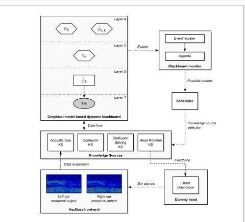
Fig. 1 shows an overview of the general system ar-chitecture that is used in this work to solve a single-source localisation task. The blackboard workspace is arranged into a hierarchy of four layers:

The first and lowest layer, denoted as the acoustic cues layer, contains observation vectors modeled as continuous, multivariate and observable random vari-ables. The observations are assembled of estimated ITDs and ILDs that can be added to the blackboard by the correspondingAcoustic Cue KS that operates on this layer. The Acoustic Cues KS takes the monau-ral left and right ear signals that were processed by the auditory front-end as inputs and estimates ITDs and ILDs independently for each frame and filterbank channel. The resulting observation vector

ok= ˆτk,1, . . . ,τˆk,N, ˆδk,1, . . . ,δˆk,N T

(1)

has2N dimensions, where ˆτk,l denotes the estimated ITD at frame index k ∈ N0 and filterbank channel l= 1, . . . , N andδˆk,l denotes the estimated ILD, re-spectively.

The central element of the second layer, which is re-ferred to as thelocation hypothesis layer, is a discrete hidden random variableφˆk which represents hypothe-ses about the possible locations of a sound source.φˆk is statistically related to the corresponding observa-tion vector described in Eq. (1). Both random vari-ables form a special case of a Bayesian network, a Gaussian Mixture Model (GMM)

p(ok|λ) =

M X

i=1

πipi(ok) (2)

composed ofM mixture components, with model pa-rametersλspecified as

λ={πi, µi,Σi}, i= 1, . . . , M.

The mixture components in (2) are modeled as D-dimensional, Gaussian distributions pi(ok) with mean vectors µi, covariance matrices Σi and mix-ture weights πi satisfying P

M

i=1πi = 1. Each GMM corresponds to a specific discrete source position in the horizontal plane φˆk,1, . . . ,φˆk,M. In this work, we restricted the number of GMMs to 72, yielding an angular resolution of 5◦ _{for the localisation} esti-mates. If new observations are added to the black-board, the GMMs are triggered to infer the poste-rior probabilities p( ˆφk,i|ok) of all possible locations. The resulting probability distribution p( ˆφk|ok) =

{p( ˆφk,1|ok), . . . , p( ˆφk,M|ok)} is then placed on the

blackboard.

(5)

Knowledge Sources

Acoustic Cue KS

Confusion KS

Head Rotation KS Confusion

Solving KS

Graphical model based dynamic blackboard

Layer 1 Layer 2 Layer 4

Event register

Agenda

Blackboard monitor

Data acquisition

Events

Scheduler

Possible actions

Knowledge source selection

Auditory front-end

Left ear monaural output

Right ear monaural output

Layer 3

Data flow

Feedback

Dummy head

Head Orientation

[image:5.595.62.543.48.484.2]

Ear signals

Figure 1. Overview of the proposed blackboard architecture. Data flow between the different components is represented by dotted arrows, whereas dashed arrows represent control commands. The different components on the blackboard are divided into continuous random variables (ellipsoid nodes), discrete random variables (rectangular nodes) and data segments (hexagonal nodes). The GMM that is used in layers 1 and 2 is illustrated by a solid arrow that represents the statistical relationship between the observation vectorsok and the discrete locationsφˆk.

probability at which one of the posterior probabili-ties p( ˆφk,i|ok)is considered as a location hypothesis. A confusion is identified if there are multiple loca-tion hypotheses within one frame. When a confusion is identified, a confusion hypothesis

ck ={φ˜k,1, . . . ,φ˜k,Q} (3)

is created which includes all Q competing locations ˜

φk,j, j= 1, . . . , Q. IfQ= 1, no confusion is detected and a relative source location hypothesis φrˆ,k is cre-ated on the fourth layer of the blackboard.

The fourth layer, denoted as theperceptual hypothe-ses layer, contains two variables ψk and φˆr,k, corre-sponding to the current head position and the esti-mated relative source position, respectively. As

scribed before, if no front/back confusion was de-tected, the estimated relative source position is di-rectly computed by the Confusion KS from the pos-terior probabilities on the second layer. If there is a remaining confusion hypothesis according to (3) on the third layer and the head has not been rotated, the

(6)

0 30 60 90 120 150 180 210 240 270 300 330 0 30 60 90 120 150 180 210 240 270 300 330

Azimuth (degrees) Azimuth (degrees)

0 0.2 0.4 0.6 0.8 1

P

ro

b

a

b

ili

ty

P

ro

b

a

b

ili

ty

True source location

Front-back confusion

Two distributions overlap at source location

Ghost

[image:6.595.62.543.51.257.2]

Probability distribution for a single source located at 30 degrees After head rotation of 30 degrees to the right

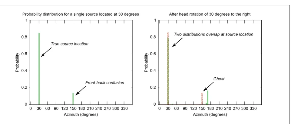
Figure 2. Illustration of front-back confusion solving. The left panel shows the probability distribution for diﬀerent positions for a source located at 30◦_{azimuth. There clearly exists a}_ghost _{at 150}◦_{azimuth. The right panel shows the} predicted location distribution in dotted lines and the actual distribution after head rotation by 10◦_{. The two distributions} overlap at 30◦_{azimuth which suggests a true source position.}

frame. If a hypothesised source position reflects a true source location, then the predicted location distribu-tion and the observed distribudistribu-tion after head rota-tion should overlap at the same locarota-tion. If this is the case, the estimated position is considered a valid rela-tive source location hypothesisφˆr,k, which is then put onto the blackboard. The corresponding confusion hy-potheses on the third layer are then discarded by the Confusion Solving KS. If the predicted and observed distributions do not match, the hypothesised location is considered aghostand the system proceeds with the next frame to gather more data before repeating the process. An example of the confusion solving process is illustrated in Figure 2.

The triggering of specific KSs is attached to certain events that are stored in an event register, which is part of the blackboard monitor. As described before, events are generated if new data is available from the auditory front-end or if specific KSs have performed certain actions on the blackboard. The blackboard monitor keeps track of the current state of the black-board and generates an agenda which contains all ac-tions that could be performed according to this state.

The agenda is then passed to the scheduler that decides which of the possible actions would be best suited given the current state of the blackboard and the task that should be accomplished. In the current system, a weight is attached to each KS represented as an integer value between 0 and 100. This weight corresponds to the importance of a specific KS for accomplishing the localisation task. Given the agenda, the scheduler executes the action that is linked to the KS with the highest weight.

4. Experiments and results

4.1. Evaluation scenario

The blackboard architecture was evaluated in a single-source localisation scenario. Here the position of the listener was assumed to be static but changes in head orientation were possible. The target sound was a static speech source, but could be located on the hor-izontal plane at an arbitrary angle between[0◦_,₃₆₀◦_] with a 5◦ _{angular resolution. Since the localisation} task was not restricted to the frontal plane, the local-isation systems were presented with potential front-back ambiguities.

7 target source positions were selected for evalua-tion:270◦_,₃₀₀◦_,₃₃₀◦_,₀◦_,₃₀◦_,₆₀◦_,₉₀◦_{. Note although} the evaluated target source positions were all on the frontal plane, the localisation systems did not have this prior knowledge and assumed an azimuth range of[0◦_,₃₆₀◦_]_{for a potential target source position.}

Two localisation conditions were evaluated. The first condition contained only the target speech source. The second condition also included a diffuse noise at a signal-to-noise ratio (SNR) of 0 dB in or-der to evaluate the noise robustness of the proposed system. In both conditions, it was assumed that the listener and the sound source were located in a free-field environment. The simulation of the scenario was generated using HRTFs [14] acquired from aKemar

dummy-head, recorded at a distance of 3 m between the head and the source.

4.2. Experimental setup

(7)

0 30 60 90 270 300 330

Target source azimuth (degrees) 0 10 20 30 40 50 L o ca lisa ti o n e rr o rs (d e g re e s)

Localisation with no noise Localisation with busy street noise at 0dB

0 10 20 30 40 50 L o ca lisa ti o n e rr o rs (d e g re e s)

0 30 60 90 270 300 330

Target source azimuth (degrees) GMM Baseline

Proposed Blackboard

[image:7.595.61.542.52.257.2]

GMM Baseline Proposed Blackboard

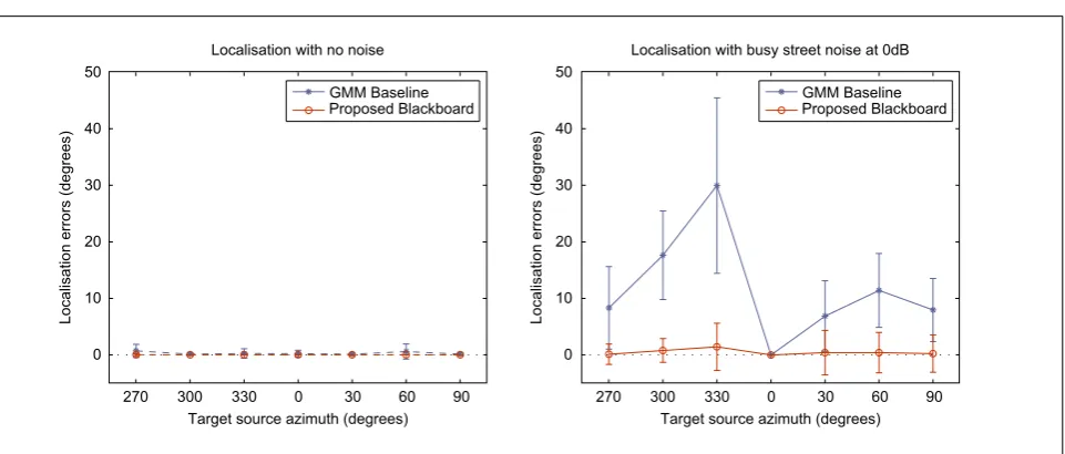
Figure 3. Mean utterance-level localisation errors of the GMM baseline and the proposed blackboard system for localising a speech source. Left: no noise was present. Right: busy street noise was present at an SNR of 0 dB. Error bars show standard deviations.

male speakers and 16 female speakers), in the form

<command> <colour> <preposition> <let-ter> <number> <adverb>_{, e.g. “place white at}

L 3 now”. The training set included 340 randomly se-lected utterances (10 utterances per speaker). They were then spatialised to produce training data for each azimuth position between [0◦_,₃₆₀◦_] _{with a} ₅◦ step. A further set of 170 utterances (5 utterances per speaker) were selected as the evaluation test set, and were spatialised to simulate the 7 target source positions described above.

The diffuse noise used in the second test condi-tion was one of the environmental sounds (“busy street”) taken from IEEE AASP CASA Challenge Dataset [19]. The noise was added to the binaural speech signals after spatialisation at an SNR of 0 dB. The peripheral processing of the auditory system was simulated by the auditory front-end described in Section 2.2, which decomposed signals arriving at both ears into 31 gammatone filterbank channels. The centre frequencies of the filterbank were equally dis-tributed on the ERB scale between 80 Hz and 8 kHz. The channel output was then halfwave-rectified and used to extract channel-dependent binaural cues. A Hann window of 20 msec was used for analysis in each frame with an overlap between successive frames of 10 msec. The ITD for each channel was estimated by choosing the maximum lag of a cross-correlation function within the range of [−1,1]msec. The chan-nel ILD was estimated by comparing the energy inte-grated across the window between the left and right ears within each channel and expressed in dB.

Two localisation systems were evaluated: a GMM-based localisation baseline and the proposed black-board system. Both systems used GMMs to model the azimuth-dependent distribution of the binaural fea-ture space consisting of ITDs and ILDs. The GMM

baseline simply selected the azimuth that has the maximum posterior given a binaural feature obser-vation as the target source position, while the black-board included top-down feedback for head rotation in order to resolve front/back ambiguities as described in Section 3. To make the two systems more com-parable both employed identical sets of GMMs. The GMMs were trained only on spatialised speech signals and no noise was included during training. No prior knowledge of source positions was used.

4.3. Results and discussion

Localisation performance of both systems was evalu-ated as utterance-level localisation errors. Utterance-level localisation errors were computed by averag-ing the minimum angular differences between the reference target position and the estimated posi-tions within each utterance. Fig. 3 shows the mean utterance-level localisation errors based on the 170 test utterances for each evaluated target position. Er-ror bars show standard deviations.

(8)

in the simulation and thus implicitly modelled by the system.

When diffuse noise was present, shown in the right panel of Fig. 3, the localisation errors of the GMM baseline increased significantly across all target posi-tions except for the 0◦ _{azimuth (average localisation} errors across all target positions:11.8◦_{). Performance} was particularly bad for the GMM baseline at azimuth positions where the front-back confusion was strong (30◦ _and ₆₀◦ _{at both sides). The performance of the} blackboard system, however, was generally robust in the presence of the diffuse noise (average localisation errors across all target positions:0.5◦_{) and was} signif-icantly better than the baseline (t-test; p < 0.001). The top-down feedback that allowed head rotation helped the system resolve most ambiguities and the improvement over the baseline was consistent across all the target positions.

5. Conclusions and future work

We have presented a general high-level framework for auditory scene analysis, which, based on a graphical-model representation, can iteratively develop an “un-derstanding” — an internal, interpretable high-level description — of an auditory scene. While results were shown for a small toy example, consisting of localisa-tion of a single acoustic source, the framework allows inference in a wide range of dynamic Bayesian net-works, supporting many types of knowledge sources and inference strategies.

Thus, a natural next step will be the integration of dynamic state-space models, describing sources not as stationary but as dynamically moving. Tracking these dynamic sources will hence become necessary. In the proposed framework, this can be achieved by incor-porating a source-type-dependent state-space model for the source position. Inference of the source posi-tion will hence be possible by developing Kalman-style filters. These, based on strategies like the unscented Kalman filter [20], can additionally include the black-board’s estimates of the uncertainties of all graphical-model variables to obtain optimal, time-varying esti-mates of all source positions.

To test feedback strategies in a controlled environ-ment, we plan to integrate our blackboard architec-ture with theBochum Experimental Feedback Testbed

(BEFT) [21], a tool that has been designed to test complex feedback strategies early in the Two!Ears

project. BEFT provides a custom-made virtual envi-ronment for visualization of XML-scripted scenes and allows the success of actual feedback strategies to be monitored in near real-time. Visual and (emulated) auditory features provided by the BEFT system core will act as input to our KSs. To that end, the testbed architecture is explicitly designed to closely approxi-mate real-life conditions: ground-truth characteristics of environmental objects are artificially degraded to

mimic weak sensor performance under adverse envi-ronmental conditions. The BEFT framework is not limited to the emulation/degradation of physical ob-ject or scenario features: specific degradation func-tions allow emulating an object classifier that provides category labels for each observed environmental entity and generates input to higher-level KSs. Further, the testbed architecture provides task stack mechanisms to control the behavior of a virtual robotic platform that explores a given scenario.

In conclusion we have shown that the extension of machine hearing systems with top-down feedback prove to be advantageous over those that are solely based on bottom-up processing. Graphical-model-based blackboard systems, as introduced in this work, are a flexible framework for further investigating the role of feedback in the context of machine hearing systems. Focusing on human perception, the black-board paradigm furthermore allows for easy integra-tion of addiintegra-tional cues like visual and tactile informa-tion, providing a powerful framework for biologically inspired computational systems.

Acknowledgement

This research has been supported by EU FET grant

Two!Ears1_{, ICT-618075. We thank Tobias May for} making the auditory front-end code available.

References

[1] A. S. Bregman: Auditory scene analysis: the per-ceptual organization of sound. Cambridge, MA: MIT Press, 1990.

[2] J. Blauert: Spatial hearing – The Psychophysics of Hu-man Sound Localization. Cambridge, MA: MIT Press, 1997.

[3] D. Wang, G. J. Brown (Eds.): Computational audi-tory scene analysis: Principles, Algorithms, and Ap-plications. IEEE Press/Wiley-Interscience.

[4] H. Wallach: The role of head movements and vestibu-lar and visual cues in sound localization. J. Exp. Psy-chol. 27(4):339–368, 1940.

[5] V. A. F. Lamme, H. SupÃĺr, H. Spekreijse: Feedfor-ward, horizontal, and feedback processing in the visual cortex. Current Opinion in Neurobiology 8(4):529–535, 1998.

[6] B. R. Schoﬁeld: Structural organization of the descend-ing auditory pathway, in: Oxford Handb. of Auditory Science, Vol. 2: The Auditory Brain. Oxford Univ. Press, New York, NY, 2009.

[7] A. Rabiee, S. Setayeshi, S. Y. Lee: CASA: Biologically Inspired Approaches for Auditory Scene Analysis. Nat-ural Intelligence: the INNS Magazine 2(1):50–58, 2012. [8] L. D. Erman, F. Hayes-Roth, V. R. Lesser, D. R. Reddy: The Hearsay-II speech understanding system: Integrating knowledge to resolve uncertainty. ACM Comput. Surv. 12(2):213–253, 1980.

(9)

[9] J. Pearl: Bayesian Networks: A Model of Self-Activated Memory for Evidential Reasoning. Proceedings of the 7th Conference of the Cognitive Science Society, Uni-versity of California, Irvine, CA. pp. 329âĂŞ-334, 1985.

[10] M. Cooke, G. J. Brown, M. Crawford, P. Green: Com-putational auditory scene analysis: listening to several things at once. Endeavour, 4, 186–190, 1993.

[11] V. R. Lesser, S. H. Nawab, F. I. Klassner: IPUS: An architecture for the integrated processing and under-standing of signals. Artiﬁcial Intelligence, 77, 129–171. [12] D. Ellis: Prediction-driven computational auditory

scene analysis. PhD Thesis, MIT, 1996.

[13] D. Godsmark, G. J. Brown: A Blackboard Archi-tecture for Computational Auditory Scene Analysis. Speech Communication, 27, 351–366, 1999.

[14] H. Wierstorf, M. Geier, A. Raake, S. Spors: A Free Database of Head-Related Impulse Response Measure-ments in the Horizontal Plane with Multiple Distances. 130th Convention of the Audio Engineering Society, 2011.

[15] T. May, S. van de Par, Armin Kohlrausch: A Prob-abilistic Model for Robust Localization Based on a Binaural Auditory Front-End. IEEE Transactions on Audio, Speech, and Language Processing 19(1):1–13, 2011.

[16] B. R. Glasberg, B. C. J. Moore: Derivation of au-ditory ﬁlter shapes from notched-noise data. Hearing research 47(1):103–138, 1990.

[17] B. C. J. Moore, B. R. Glasberg, T. Baer: A model for the prediction of thresholds, loudness and partial loudness. J. Audio Eng. Soc., vol. 45, pp. 224–240, 1997.

[18] M. Cooke, J. Barker, S. Cunningham, X. Shao: An audio-visual corpus for speech perception and auto-matic speech recognition. Journal of the Acoustical Society of America, 120, 12421–24, 2006.

[19] D. Giannoulis, E. Benetos, D. Stowell, M. D. Plumb-ley: IEEE AASP Challenge on Detection and Classiﬁ-cation of Acoustic Scenes and Events - Public Dataset for Scene Classiﬁcation Task, Queen Mary University of London, 2012.

[20] S. J. Julier, J. K. Uhlmann: A new extension of the Kalman ﬁlter to nonlinear systems. Int. Symp. Aerospace/Defense Sensing, Simul. and Controls 3: 182, 1997