Asymmetric quantum hypothesis testing with Gaussian states

This is a repository copy of

Asymmetric quantum hypothesis testing with Gaussian states

.

White Rose Research Online URL for this paper:

http://eprints.whiterose.ac.uk/81539/

Version: Published Version

Article:

Spedalieri, Gaetana and Braunstein, Samuel Leon orcid.org/0000-0003-4790-136X (2014)

Asymmetric quantum hypothesis testing with Gaussian states. Physical Review A. 052307.

ISSN 1094-1622

https://doi.org/10.1103/PhysRevA.90.052307

eprints@whiterose.ac.uk https://eprints.whiterose.ac.uk/ Reuse

Items deposited in White Rose Research Online are protected by copyright, with all rights reserved unless indicated otherwise. They may be downloaded and/or printed for private study, or other acts as permitted by national copyright laws. The publisher or other rights holders may allow further reproduction and re-use of the full text version. This is indicated by the licence information on the White Rose Research Online record for the item.

Takedown

If you consider content in White Rose Research Online to be in breach of UK law, please notify us by

Asymmetric quantum hypothesis testing with Gaussian states

Gaetana Spedalieri and Samuel L. Braunstein

Department of Computer Science, University of York, York YO10 5GH, United Kingdom

(Received 3 July 2014; published 6 November 2014)

We consider the asymmetric formulation of quantum hypothesis testing, where two quantum hypotheses have different associated costs. In this problem, the aim is to minimize the probability of false negatives and the optimal performance is provided by the quantum Hoeffding bound. After a brief review of these notions, we show how this bound can be simplified for pure states. We then provide a general recipe for its computation in the case of multimode Gaussian states, also showing its connection with other easier-to-compute lower bounds. In particular, we provide analytical formulas and numerical results for important classes of one- and two-mode Gaussian states.

DOI:10.1103/PhysRevA.90.052307 PACS number(s): 03.67.Hk,89.70.Cf,03.65.Ta

I. INTRODUCTION

Quantum hypothesis testing (QHT) is a fundamental topic in quantum information theory [1,2], playing a nontrivial role in protocols of quantum communication and quantum cryptography [3,4]. The typical formulation of QHT is given in terms of quantum state discrimination [5–8], where a certain number of generally nonorthogonal quantum states (the quantum hypotheses) have to be discriminated by means of a quantum measurement. In particular, the simplest scenario regards the statistical discrimination between two nonorthog-onal quantum states, corresponding to the “null” and the “alternative” quantum hypotheses, occurring with some a priori probabilities. In symmetric testing, these hypotheses have the same cost [6–8] and the goal is to minimize the mean error probability of confusing them by suitably optimizing the quantum measurement.

For such a basic problem, we know closed analytical formulas identifying both the minimum error probability, given by the Helstrom bound [6], and the optimal quantum detection, expressed in terms of the Helstrom matrix [6]. Furthermore, we can also use an easier-to-compute bound which becomes tight in asymptotic conditions. This is the recently introduced quantum Chernoff bound [9], for which we know simple formulas in the case of multimode Gaussian states [10] (i.e., those states with Gaussian Wigner function [5]).

In this paper, we consider asymmetric QHT, where two quantum hypotheses have different associated costs [6–8]. In this approach, we aim to minimize the probability that the alternative hypothesis is confused for the null hypothesis, an error which is known as “false negative.” This minimization has to be done by suitably constraining the probability of another possible error, known as a “false positive,” where the null hypothesis is confused for the alternative hypothesis. This is clearly the best approach, for instance, in medical-type testing, where the null hypothesis typically represents absence of a disease, while the alternative corresponds to the presence of a disease.

Asymmetric QHT is typically formulated as a multicopy discrimination problem, where a large number of copies of the two possible states are prepared and subjected to a collective quantum measurement. From this point of view, the aim is to maximize the error exponent describing the exponential decay of the false negatives, while placing a reasonable constraint

on the false positives. For this calculation, we can rely on two mathematical tools. The first is the quantum relative entropy [5] between the two states, while the other is the recently introduced quantum Hoeffding bound (QHB) [11], which performs the optimization of the error exponent while providing a better control on the false positives.

In this work, we start by giving some basic notions on asymmetric QHT and briefly reviewing the QHB, also showing how its computation simply reduces to the quantum fidelity [12] in the presence of pure states. Then, we provide a general recipe for computing this bound in the case of multimode Gaussian states, for which it can be expressed in terms of their first- and second-order statistical moments. In the general multimode case, we derive a relation between the QHB and other easier-to-compute bounds, which are based on well-known mathematical inequalities. Finally, we derive analytical formulas and numerical results for the most important classes of one-mode and two-mode Gaussian states. By developing the theory of asymmetric QHT for Gaussian states, our work could be useful in tasks and protocols involving Gaussian quantum information [5], including tech-nological applications of quantum channel discrimination (e.g., quantum illumination [13,14] or quantum reading [15–18]) where we are interested in increasing our ability to accept one specific quantum hypothesis.

II. BRIEF REVIEW OF ASYMMETRIC TESTING

A. Basic formulation

In binary QHT we consider a quantum system which is prepared in some unknown quantum stateρ, which can beρ0

orρ1. For instance, we can imagine one party, say Alice, who

prepares such a system. This system is then passed to Bob, who does not know which choice Alice has made. Thus, Bob must decide between the following two hypotheses:

Null hypothesisH0:ρ=ρ0, (1)

Alternative hypothesisH1:ρ=ρ1. (2)

GAETANA SPEDALIERI AND SAMUEL L. BRAUNSTEIN PHYSICAL REVIEW A90, 052307 (2014)

always reduce his measurement to be a dichotomic POVM

{k} with k=0,1 [6]. The outcome k=0, with POVM

operator0, is associated with the null hypothesesH0, while

the other outcomek₌1, with POVM operator1=I−0,

is associated with the alternative hypothesisH1.

Since the two quantum states ρ0 and ρ1 are generally

nonorthogonal, there is a nonzero error probability to confuse the two hypotheses. We can identify two different types of error: Type-I and type-II errors, with associated conditional error probabilities. By definition, the type-I error, also known as a “false-positive,” is where Bob accepts the alternative hypothesis H1 when the null hypothesisH0 holds. We have

a corresponding error probability expressed by

α:=p(H1|H0)=Tr(1ρ0). (3)

Then, the type-II error or “false negative” is where Bob accepts the null hypothesisH0when the true hypothesis is the

alternativeH1. This error occurs with conditional probability,

β:=p(H0|H1)=Tr(0ρ1). (4)

Note that we can introduce other probabilities, but they are fully determined byαandβ. For instance, we may also consider the “specificity” or “true negativity” of the test which is the success probability of identifying the null hypothesis, i.e., p(H0|H0) which is simply given by 1−α. Similarly,

we may also consider the “sensitivity” or “true positivity” of the test which is the success probability of identifying the alternative hypothesis, i.e.,p(H1|H1)=1−β.

The costs associated with the two types of error can be very different especially in the medical and histological settings. For instance, in a medical test,H0is typically associated with

no illness, while H1 with the presence of the disease. It is

therefore clear that we would like to have tests where the false-negative probability (or rate) β is the lowest possible, so that ill patients are not diagnosed as healthy. For this reason, in a medical setting, hypothesis testing is almost always asymmetric, meaning that we aim to minimize one of the two conditional error probabilities.

B. Multicopy formulation

In general we can formulate the problem of QHT as an M-copy discrimination problem [7,8]. This means that Alice hasM quantum systems which are prepared in two possible multicopy states,

H0:ρ =ρ0⊗M =ρ0⊗ · · · ⊗ρ0,

(5) H1:ρ =ρ1⊗M =ρ1⊗ · · · ⊗ρ1.

These systems are passed to Bob who performs a collective measurement on them. As before, this general POVM can be chosen to be dichotomic{0,1}with1=I−0.

The error probabilities now depend on the number of copies M. In particular, the probability of false positives is given by

αM :=p(H1|H0)=Tr

1ρ0⊗M

, (6)

and the probability of false negatives is

βM :=p(H0|H1)=Tr0ρ1⊗M

. (7)

In the limit of a large number of copies (M_≫1), these probabilities go to zero exponentially, i.e., we have

αM ≃ 1₂e−αRM, βM ≃ 1₂e−βRM, (8)

where the coefficients,

αR = − lim M→+∞

1

MlnαM, (9)

βR = − lim M→+∞

1

MlnβM, (10) are called the “error exponents” or “rate limits” [11].

Bob’s aim is to maximize the error exponentβR, so that

the error probability of false negatives βM has the fastest

exponential decay to zero. This must be done while controlling the rate of false positives. Here a well-known result is the “quantum Stein lemma” [11] which connects βR with the

quantum relative entropy between the single-copy statesρ0and

ρ1. For a large number of copiesM≫1, there is a dichotomic

POVM such that the error probability of the false positives is bounded,

αM ε for any 0< ε <1, (11)

and the error probability of false negatives goes to zero with the error exponent,

βR=S(ρ0||ρ1)=Trρ0(lnρ0−lnρ1). (12)

More powerfully, we may use the notion of the QHB [11]. ForM_≫1, there is a dichotomic POVM such that the error exponent of false positives is lower bounded by a positive parameter,

αRr for any r >0, (13)

and the error exponent of false negatives satisfies

βR =H(r), (14)

whereH(r)0 is the QHB defined by

H(r) := sup

0s<1

P(r,s), P(r,s) :=−rs−lnCs

1₋s , (15)

where

Cs :=Tr

ρ₀sρ₁1−s

(16)

is the “soverlap” between the single-copy states ρ0 andρ1.

Note that the quantum Hoeffding bound enforces a stronger constraint on false positives, since these are bounded at the level of the error exponent and not at the level of the error probability as happens for the quantum relative entropy bound.

III. ASYMMETRIC TESTING WITH PURE STATES

Asymmetric testing becomes very simple when one of the states (or both) is pure. In this case, we can in fact relate the QHB to the quantum fidelity between the two states.

Let us start by considering the case where only one of the states is pure, e.g.,ρ0= |ψ0ψ0|. We can write [19]

inf

s Cs =F(|ψ0, ρ1), (17)

where F is the fidelity between|ψ0 andρ1. Equation (17)

impliesCsF. By using the latter inequality in Eq. (15), we

derive the fidelity bound,

H(r)HF(r) := sup

0s<1

−rs₋lnF

1−s . (18)

This bound can be further simplified by explicitly perform-ing the maximization with regard to the parameters. After a simple calculation we find

HF(r)=

ln1

F, for r ln

1

F,

+∞, for r<ln_F1, (19)

which depends on the comparison between the parameterr and the fidelityF of the two states.

More specifically, in the discrimination of two pure states, we find that the previous fidelity bound becomes tight,

H(r)=HF(r). (20)

In fact, for pure statesρ0= |ψ0ψ0|andρ1= |ψ1ψ1|, and

for any 0< s <1, we can write

Cs =Tr(|ψ0ψ0|s|ψ1ψ1|1−s)=Tr(|ψ0ψ0|ψ1ψ1|)

= |ψ0|ψ1|2=F(|ψ0,|ψ1). (21)

Therefore we can replace lnCs =lnFin the QHB of Eq. (15),

which implies Eq. (20) [20].

IV. ASYMMETRIC TESTING WITH GAUSSIAN STATES

A. Basics of bosonic systems and Gaussian states

A bosonic system ofnmodes is a quantum system described by a tensor product Hilbert space H⊗n _{and a vector of}

quadrature operators [21,22]:

ˆxT :=( ˆq1,pˆ1, . . . ,qˆn,pˆn). (22)

These operators satisfy the vectorial commutation rela-tions [23],

[ˆx,ˆxT] :=ˆxˆxT −(ˆxˆxT)T =2i, (23)

whereis the symplectic form, defined as

:= n

k=1

0 1

−1 0

. (24)

Correspondingly, a real matrixSis called “symplectic” when it preservesby congruence, i.e.,SST

=.

By definition, we say that a bosonic stateρis “Gaussian” when its phase-space Wigner representation is Gaussian [5]. In such a case, we can completely describe the state by means of its first- and second-order statistical moments. These are the mean value or displacement vector ¯x:=Tr(ˆxρ), and the covariance matrix (CM)Vwith the generic element,

Vij =1₂Tr({xˆi,xˆj}ρ)−x¯ix¯j, (25)

where _{,_} denotes the anticommutator. The CM is a 2n_× 2nreal symmetric matrix, which must satisfy the uncertainty principle [5],

V+i0. (26)

An important tool in the manipulation of Gaussian states is Williamson’s theorem [5]: For any CMV, there is a symplectic

matrixSsuch that

V₌SWST, (27)

where

W= n

k=1

νkI, I:=

1 0

0 1

. (28)

The matrix W is the “Williamson form” of V, and the set

{ν1,· · · ,νn} is the “symplectic spectrum” of V. According

to the uncertainty principle, each symplectic eigenvalue must satisfy the conditionνk 1, withνk=1 for allkif and only

if the Gaussian state is pure.

B. Computation of the quantum Hoeffding bound

Our goal is to find a general recipe for the calculation of the QHB for Gaussian states. We start from the general formula in Eq. (15) involving the logarithm of thesoverlapCsdefined

in Eq. (16). Given twon-mode Gaussian states,ρ0andρ1, we

can write an explicit Gaussian formula for the s overlap in terms of their statistical moments (¯x0,V0) and (¯x1,V0). This

is given by [10,19]

Cs =

s √

dets

exp

−d T

−s1d

2 , (29)

whered:₌¯x0−¯x1is the difference between the mean values,

whilesandsdepends on the CMsV0andV1. In particular,

introducing the two real functions,

Gs(x) :=

2s

(x₊1)s_−(x−1)s, (30)

s(x) :=

(x₊1)s

+(x₋1)s

(x₊1)s

−(x₋1)s, (31)

we can write the formulas,

s :=2nnk=1Gs

ν_k0G1−s(νk1), (32)

and

s:=S0

⊕nk=1 s

ν_k0I

ST₀

+S1

⊕nk=1 1−s

ν_k1IST1, (33)

where _{ν_k0_}and _{ν_k1_} are the symplectic spectra of the two states, with S0 andS1 being the symplectic matrices which

diagonalize the two CMs according to Williamson’s theorem, i.e.,

V0 =S0

⊕nk=1ν 0

kI

ST₀, V1 =S1

⊕nk=1ν 1

kI

ST₁. (34)

Substituting Eq. (29) into Eq. (15) corresponds to explicitly computing the logarithmic term lnCs, yielding

lnCs =lns−1₂

ln dets+dT−s1d

. (35)

In particular for zero-mean Gaussian states we haved=0 and the previous expression simplifies to

GAETANA SPEDALIERI AND SAMUEL L. BRAUNSTEIN PHYSICAL REVIEW A90, 052307 (2014)

C. Other computable bounds

Note that computing thes overlapCs and its logarithmic

form lnCs could be difficult due to the presence of the

symplectic matrices,S0 andS1, in the term s in Eq. (33).

A possible solution is to compute an upper bound, known as the “Minkowski bound,” which is based on the Minkowski determinant inequality [24] and depends only on the two symplectic spectra [10]. Specifically, we haveCsMs, where

Ms :=4n

n

k=1

s

ν_k0,ν_k1₊

n

k=1

1−s

ν_k1,ν_k0

−n

, (37)

and

s(x,y) := {[(x+1)s+(x−1)s]

×[(y₊1)1−s−(y₋1)1−s]}1/n. (38) Another easy-to-compute upper bound is the “Young bound” Ys, which is based on Young’s inequality [25] and satisfies

CsMsYs, (39)

where [10]

Ys:=2n n

k=1

Ŵs

ν_k0Ŵ1−s

ν_k1, (40)

and

Ŵs(x) :=[(x+1)2s−(x−1)2s]−

1

2. (41)

Taking the negative logarithm of Eq. (39), we can write the following inequality for the QHB:

H(r)HM(r)HY(r), (42)

where

HM(r) := sup

0s<1

−rs₋lnMs

1−s , (43)

HY(r) := sup

0s<1

−rs₋lnYs

1−s . (44)

In the specific case where one of the two Gaussian states is pure, we can compute their fidelity F and apply the upper bound given in Eqs. (18) and (19), which becomes tight when both states are pure [see Eq. (20)]. In particular, for two multimode Gaussian states ρ0= |ψ0ψ0| and ρ1, we

can easily write their fidelity F in terms of the statistical moments [19]:

F ₌ 2

n √

detLexp

−d T_L−1_d

2

, (45)

whereL:=V0+V1. As a result, we can use Eq. (19) with

ln 1 F =

1 2

ln

detL

4n

+dTL−1d . (46)

V. DISCRIMINATION OF ONE-MODE GAUSSIAN STATES

In this section, we examine the case of one-mode Gaussian states. This means we fix n₌1 in the previous formulas of Sec. IV, with matrices becoming 2×2, vectors becoming two-dimensional, and symplectic spectra reducing to a single

eigenvalue. For instance, the s overlap can be more simply computed using the expressions,

s =2Gs(ν0)G1₋s(ν1), (47)

s= s(ν0)S0ST0 + 1−s(ν1)S1ST1. (48)

In particular, here we shall derive the analytic formulas for the QHB for two important classes: coherent states (in Sec.V A) and thermal states (in Sec.V B).

A. Asymmetric testing of coherent amplitudes

The expression of the QHB is greatly simplified in the case of one-mode coherent states ρ0= |α0α0| and ρ1=

|α1α1|. Since both states are pure, the QHB is equal to the

fidelity bound in Eq. (19), i.e.,H(r)₌HF(r). Therefore, it

is sufficient to compute the fidelity between the two coherent states, which is given by

F _{= |}α0|α1|2=e−|α0−α1| 2

, (49)

so that ln_F1 = |α0−α1|2:=σ, and we can write

H(r)=

σ, for rσ,

+∞, for r< σ. (50)

Assuming that we impose a good control on the rate of false positives (so thatrσ), then the error exponent for the false negatives is simply given byH(r)=σ. More explicitly, this corresponds to an asymptotic error rate,

βM =

1 2e

−Mσ =F

M

2 . (51)

Note that if we have poor control on the rate of false positives, i.e., r < σ, then the QHB H(r) is infinite. This means that the probability of false negativesβM goes to zero

superexponentially, i.e., more quickly than any decreasing exponential function.

B. Asymmetric testing of thermal noise

In this section we derive the QHB for one-mode thermal statesρ0=ρth(ν0) andρ1=ρth(ν1), with variances equal to

ν0andν1, respectively (in our notation,ν₌2 ¯n₊1, where ¯nis the mean number of thermal photons). These Gaussian states have zero mean (¯x0=¯x1=0) and CMs in the Williamson

formV0 =ν0IandV1=ν1I(so thatS0 =S1=I). Thus, we

can write

s =εsI, εs := s(ν0)+ 1−s(ν1), (52)

and derive

Cs =

s

εs =

2 (ν0

+1)s_(ν1

+1)1−s −(ν0

−1)s_(ν1

−1)1−s.

(53)

This is thesoverlap to be used in the QHB of Eq. (15). Given two arbitraryν0_{1 andν}1_{1, the maximization}

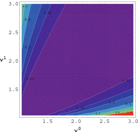
in Eq. (15) can be done numerically. The results are shown in Fig.1for thermal states with variances up to 3 vacuum units (equivalent to 1 mean thermal photon). From the figure we can see an asymmetry with respect to the bisectorν0₌ν1which is a consequence of the asymmetric nature of the hypothesis test.

0.01 0.01

0.05 0.05

0.1 0.1

0.2 0.2

0.3 0.3

0.4 0.5

1.5 2.0 2.5 3.0

1.5 2.0 2.5 3.0

Ν

Ν

FIG. 1. (Color online) We plot the QHB associated with the discrimination of two thermal states:ρth(ν0_{) as null hypothesis, and}

ρth(ν1_{) as alternative hypothesis. We consider low thermal variances} 1< ν0_,ν1_{3 and we have setr}

=0.1 for the false positives.

The bottom-right part of the figure is related to the minimum probability of confusing a nearly vacuum state (ν1_≃1) with a thermal state having one average photon (ν0

≃3). By contrast, the top-left part of the figure is related to the probability of confusing a thermal state having one average photon (ν1

≃3) with a nearly vacuum state (ν0_≃1). These probabilities are clearly different.

We are able to derive a simple analytical result when we compare a thermal state with the vacuum state. Let us start by considering the vacuum state to be the null hypothesis (ν0₌1) while the thermal state is the alternative hypothesis (ν1:=ν >1). In this specific case, we find

lnCs =(1−s) ln

2 1+ν

, (54)

and we get

P(r,s)₌ln

1+ν 2

− rs

1−s. (55)

Sinceνis a constant, the maximization ofPover 0s <1 corresponds to minimizing the functionrs(1−s)−1, whose minimum occurs ats₌0. As a result, we have

H(r)=P(r,0)=ln

1+ν 2

.

Sinceν₌2 ¯n₊1, we can write the QHB in terms of the mean number of thermal photons, i.e.,

H(r)=ln( ¯n₊1). (56)

This is the optimal error exponent for the asymptotic proba-bility of false negatives, i.e., of confusing a thermal state with the vacuum state.

Let us now consider the thermal state to be the null hypoth-esis (ν0_:

=ν >1) while the vacuum state is the alternative hypothesis (ν1

=1). In this case, we derive

P(r,s)₌ s 1−s

ln

1+ν

2

−r , (57)

which leads to the following expression for the QHB:

H(r)=

0 for rln1+ν

2

,

+∞ for r<ln1+ν

2

. (58)

This is related to the minimum probability of confusing the vacuum state with a thermal state. Note that this is very different from Eq. (56).

VI. DISCRIMINATION OF TWO-MODE GAUSSIAN STATES

In this section we consider two important classes of two-mode Gaussian states. The first is the class of Einstein-Podolsky-Rosen (EPR) states, also known as two-mode squeezed vacuum states. The second (broader) class is that of two-mode squeezed thermal (ST) states, for which the computation of the QHB is numerical.

A. Asymmetric testing of EPR correlations

The expression of the QHB in the case of EPR states is easy to derive. Since EPR states are pure, the QHBH(r) is given byHF(r) of Eq. (19). As a result, we need only to compute

the fidelity between the two states. An EPR state has zero mean and CM,

VEPR(μ)=

μI μ2

−1Z

μ2_{−1Z μI}

, (59)

withμ1,Iis the 2×2 identity matrix, and

Z:=

1 0

0 −1

. (60)

Given two EPR states with parametersμ0andμ1, their fidelity

is computed via Eq. (45), yielding

F _{= √}4

detL, (61)

where L₌VEPR(μ0)+VEPR(μ1). After simple algebra, we

find

F ₌ 2

1+μ0μ1−

μ2₀₋1μ2₁₋1

, (62)

to be used in Eq. (19).

B. Squeezed thermal states

In this section we consider symmetric ST states ρ(μ,c), which are Gaussian states with zero mean and CM,

VST(μ,c)=

μI cZ cZ μI

, (63)

GAETANA SPEDALIERI AND SAMUEL L. BRAUNSTEIN PHYSICAL REVIEW A90, 052307 (2014)

0.1 0.2

0.3

0.4

0.5

0.6 0.7

0.8 1

1.0 1.5 2.0 2.5 3.0

0.00 0.05 0.10 0.15 0.20

Μ

r

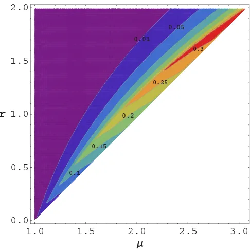
FIG. 2. (Color online) Asymmetric discrimination between the thermal stateρ0=ρ(μ,0) and the ST stateρ1=ρ(μ,μ−1) with maximal separable correlations. We plot the QHB as a function of the thermal varianceμand the false-positive parameterr. As we can see the QHB improves for lowerrand for higherμ.

because they are invariant under permutation of the two modes [28].

Note that, for c₌0, we have no correlations, and the ST state is a tensor product of thermal states, i.e.,ρ(μ,0)₌ ρth(μ)⊗2. Forc=

μ2

−1 the correlations are maximal, and the ST state becomes an EPR state, i.e., ρ(μ,μ2

−1)=

ρEPR(μ). Finally, forc=μ−1, we have maximal separable

correlations. In other words,ρ(μ,μ₋1) is the separable ST state with the strongest correlations (e.g., highest discord).

The symplectic decomposition of a symmetric ST state is known. From the CM of Eq. (63), one can check that the symplectic spectrum is degenerate and given by the single eigenvalue,

ν₌μ2_−c2_{. (64)}

The symplectic matrixSwhich diagonalizesVST(μ,c) in the

Williamson formν(I⊕I) is given by

S₌

ω₊I ω₋Z ω₋Z ω₊I

, (65)

where

ω_±:=

μ_±ν

2ν . (66)

As a result, thesoverlap between two symmetric ST states, ρ0andρ1, can be computed using the simplified formulas,

s =4G2s(ν

0

)G2_1−s(ν1), (67)

s = s(ν0)S0ST0 + 1−s(ν1)S1ST1, (68)

whereν0(ν1) is the degenerate eigenvalue ofρ0(ρ1), computed

according to Eq. (64), and S0 (S1) is the corresponding

0.01

0.05

0.1 0.15

0.2 0.25

0.3

1.0 1.5 2.0 2.5 3.0

0.0 0.5 1.0 1.5 2.0

Μ

r

FIG. 3. (Color online) Asymmetric discrimination between the thermal stateρ0=ρ(μ,0) and the EPR stateρ1=ρEPR(μ). We plot the QHB as a function of the thermal varianceμand the false-positive parameterr. The QHB improves for lowerr and for higher μ. In particular, there is a threshold value after which the QHB becomes infinite (white region).

diagonalizing symplectic matrix, computed according to Eqs. (65) and (66).

Let us start with simple cases involving the asymmetric testing of correlations with specific ST states. First we consider the asymmetric discrimination between the uncor-related thermal state ρ0=ρ(μ,0) as null hypothesis and

the correlated (but separable) ST state ρ1=ρ(μ,μ−1)

as alternative hypothesis. A false negative corresponds to concluding that there are no correlations where they are actually present [29]. It is straightforward to derive their degenerate symplectic eigenvalues which are simplyν0

=μ andν1₌√2μ₋1. Then, we haveS0=I⊕I, whileS1 can

be easily computed from Eqs. (65) and (66). By substituting these into Eqs. (67) and (68), we can compute thesoverlap Cs =s/√detsand therefore the QHBH(r) via Eq. (15).

The results are plotted in Fig. 2, for values of thermal variance μ up to 3 (i.e., from zero to 1 mean photon) and small values of the parameter r, bounding the rate of false positives. As expected, the QHB improves for decreasingrand increasingμ.

Now let us consider the asymmetric discrimination between ρ0=ρ(μ,0) and the EPR state ρ1=ρEPR(μ), i.e., the most

correlated and entangled ST state [29]. Thanks to the simple symplectic decomposition of the EPR state (ν1₌1), we can further simplify the previous Eqs. (67) and (68) and write

s =4G2s(μ), s = s(μ)(I⊕I)+VEPR(μ), (69)

withVEPR(μ) being given by Eq. (59). As before, we compute

the QHB which is plotted in Fig.3, for 1μ3 andr2. As expected the QHB improves for decreasingrand increasing μ. Note a discontinuity identifying two regions, one where the

0.01 0.01

0.05 0.05

0.1 0.1

0.15 0.15

0.2 0.2

0.25 0.25

0.3 0.3

0.4 0.4

0.5 0.6

0.7 0.8

0.0 0.5 1.0 1.5 2.0 0.0

0.5 1.0 1.5 2.0

c

c

FIG. 4. (Color online) Asymmetric discrimination between two ST states with the same thermal variance (μ₌3) but different correlationsc0andc1. Settingr=0.1, we plot the QHB as a function ofc0andc1. We can see that the QHB increases orthogonally to the bisectorc0=c1.

QHB is finite, and the other where it is infinite (white region in the figure).

In fact, by expanding the termP(r,s) in Eq. (15) fors_→ 1−_{, then we find}

P(r,s)≃ N

s₋1 +O(s−1), (70)

where

N:=r₋ln

1+3μ2

4

. (71)

For values ofr andμsuch thatN >0, we find that the term P(r,s) diverges at the border, making the QHB infinite. For a givenr, this happens when

μ >μ˜(r) :₌

4er₋₁

3 . (72)

Finally, we consider the most general scenario in the asymmetric testing of correlations with ST states. In fact, we consider two generic ST states,ρ(μ,c0) andρ(μ,c1), with the

same thermal noise but differing amounts of correlation. For this computation, we use Eqs. (64)–(66) with c₌c0 or c1,

to be replaced in Eqs. (67) and (68), therefore deriving the s overlap and the QHB. At small thermal variance (μ₌3) and for the numerical valuer₌0.1, we plot the QHB as a function of the correlation parameters c0 andc1. As we can

see from Fig.4, the QHB is not symmetric with respect to the bisector c0=c1 (where it is zero) and increases away from

this line.

VII. CONCLUSION

In this work we have considered the problem of asymmetric quantum hypothesis testing by adopting the recently developed tool of the quantum Hoeffding bound (QHB). After a brief review of these notions, we have shown how the QHB can be simplified in some cases (pure states) and estimated using other easier-to-compute bounds based on simple algebraic inequalities.

In particular, we have applied the theory of asymmetric testing to multimode Gaussian states, providing a general recipe for the computation of the QHB in the Gaussian setting. Using this recipe, we have found analytic formulas and shown numerical results for important classes of one-mode and two-mode Gaussian states. In particular, we have studied the behavior of the QHB in the low energy regime, i.e., considering Gaussian states with a small average number of photons.

Our results could be exploited in protocols of quantum information with continuous variables. In particular, they could be useful for reformulating Gaussian schemes of quantum state discrimination and quantum channel discrimination in such a way as to give more importance to one of the quantum hypotheses. This asymmetric approach could be the most suitable in the development of quantum technology for medical applications.

ACKNOWLEDGMENTS

This work has been supported by EPSRC (Grant No. EP/J00796X/1). G.S. has been supported by an EPSRC DTA grant. The authors thank C. Ottaviani and S. Pirandola for enlightening discussions.

[1] M. M. Wilde, Quantum Information Theory (Cambridge University Press, Cambridge, 2013).

[2] M. A. Nielsen and I. L. Chuang,Quantum Computation and Quantum Information(Cambridge University Press, Cambridge, 2000).

[3] C. Silberhorn, T. C. Ralph, N. Lutkenhaus, and G. Leuchs,Phys. Rev. Lett.89,167901(2002).

[4] A. M. Lance, T. Symul, V. Sharma, C. Weedbrook, T. C. Ralph, and P. K. Lam,Phys. Rev. Lett.95,180503(2005).

[5] C. Weedbrook, S. Pirandola, R. Garcia-Patron, N. J. Cerf, T. C. Ralph, J. H. Shapiro, and S. Lloyd,Rev. Mod. Phys.84,621

(2012).

[6] C. W. Helstrom,Quantum Detection and Estimation Theory,

Mathematics in Science and Engineering, Vol. 123 (Academic Press, New York, 1976).

[7] A. Chefles,Contemp. Phys.41,401(2000).

GAETANA SPEDALIERI AND SAMUEL L. BRAUNSTEIN PHYSICAL REVIEW A90, 052307 (2014) [9] K. M. R. Audenaert, J. Calsamiglia, R. Mu˜noz-Tapia, E. Bagan,

L. Masanes, A. Acin, and F. Verstraete, Phys. Rev. Lett.98,

160501(2007).

[10] S. Pirandola and S. Lloyd, Phys. Rev. A 78, 012331

(2008).

[11] K. M. R. Audenaert, M. Nussbaum, A. Szkola, and F. Verstraete, Commun. Math. Phys. 279, 251

(2008).

[12] R. Jozsa,J. Mod. Opt.41,2315(1994).

[13] S.-H. Tan, B. I. Erkmen, V. Giovannetti, S. Guha, S. Lloyd, L. Maccone, S. Pirandola, and J. H. Shapiro,Phys. Rev. Lett. 101,253601(2008).

[14] S. Lloyd,Science321,1463(2008).

[15] S. Pirandola, Phys. Rev. Lett. 106, 090504

(2011).

[16] S. Pirandola, C. Lupo, V. Giovannetti, S. Mancini, and S. L. Braunstein, New J. Phys. 13, 113012

(2011).

[17] G. Spedalieri, C. Lupo, S. Mancini, S. L. Braunstein, and S. Pirandola, Phys. Rev. A 86, 012315

(2012).

[18] C. Lupo, S. Pirandola, V. Giovannetti, and S. Mancini, Phys. Rev. A87,062310(2013).

[19] G. Spedalieri, C. Weedbrook, and S. Pirandola,J. Phys. A: Math. Theor.46,025304(2013).

[20] We can write H(r)₌max_{P(r,0),sup_0<s<1P(r,s)_}, where

P(r,0)_{= −}lnC0=0 can be neglected and sup

0<s<1

P(r,s)₌ sup 0<s<1

−rs₋lnF

1₋s

=

ln1

F for rln

1

F,

+∞ for r<ln1

F .

[21] S. L. Braunstein and P. van Loock,Rev. Mod. Phys.77,513

(2005).

[22] S. L. Braunstein and A. K. Pati, Quantum Information with Continuous Variables(Kluwer Academic, Dordrecht, 2003). [23] More generally, for any two vectorial operators aand b, we

can express their commutation relations in the compact form [a,bT_{] :}

=abT

−(baT₎T_.

[24] R. Bhatia,Matrix Analysis(Springer-Verlag, New York, 1997). [25] W. H. Young,Proc. R. Soc. London, Ser. A87,331(1912). [26] S. Pirandola, A. Serafini, and S. Lloyd,Phys. Rev. A79,052327

(2009).

[27] S. Pirandola,New J. Phys.15,113046(2013). [28] Extension to asymmetric ST states is only technical.

[29] For brevity we do not consider the other case where the ST state is the null hypothesis and the thermal state is the alternative hypothesis. This case is included in our final analysis for generic ST states.