Algebraic generation of single domain computational grid for twin screw machines. Part I. Implementation

City, University of London Institutional Repository

Citation

:

This is the accepted version of the paper.

This version of the publication may differ from the final published

version.

Permanent repository link:

Link to published version

:

Copyright and reuse:

City Research Online aims to make research

outputs of City, University of London available to a wider audience.

Copyright and Moral Rights remain with the author(s) and/or copyright

holders. URLs from City Research Online may be freely distributed and

linked to.

City Research Online: http://openaccess.city.ac.uk/ [email protected]

1

Algebraic Generation of Single Domain Computational Grid for Twin Screw Machines

Part I – Implementation

Sham Rane*, Ahmed Kovacevic

Centre for Compressor Technology, City, University of London, EC1V 0HB, London, U.K. Email: [email protected] , Tel: +44(0) 20 70408795,

* Corresponding Author

Abstract

Special attention is required for generation of computational grids in highly deforming working chambers of twin screw machines for 3D CFD calculations. Two approaches for customised grid generation are practically available. The first is an algebraic grid generation and the second is a differential decomposition method. This paper reports on new developments in the algebraic approach that has the advantages associated with both algebraic and differential methods. Two control functions are introduced for regularisation of the initial algebraic distribution. One is based on an analytical control function in transformed coordinate system while the other uses background blocking structure in order to guide the initial algebraic distribution towards a single computational mesh. This paper presents implementation and grid characteristics of these new functions. Developed grids have been tested and results from flow calculations on a dry air compressor have been validated in part II [29] of the paper.

It was possible to achieve two distinct characteristics desirable in a twin screw rotor domain mesh. Firstly, it is possible to independently control grid refinement in the interlobe region thereby providing better accuracy in representation of the leakage gaps. Secondly and most importantly, it is possible now to eliminate the non-conformal interface between the two rotor domains thereby producing a single domain structured grid for the rotors, while still maintaining the fully hexahedral cell topology. An improvement in the global orthogonality of the cells was achieved. Despite of a decrement in the Face warp quality, aspect ratio of cells retained similar scale.

Keywords

Computational Fluid Dynamics, Algebraic Grid Generation, Twin Screw Compressors, Deforming Grid, Positive Displacement Compressors.

Nomenclature

𝐴𝐴𝑠𝑠𝑠𝑠 - amplitude of the sine function 𝑥𝑥,𝑦𝑦 - Cartesian coordinates

𝑛𝑛𝑠𝑠𝑠𝑠 - frequency of the sine function 𝑟𝑟,𝜃𝜃 - polar coordinates of a point

2 𝑡𝑡 - period of the sine function 𝑆𝑆_𝑖𝑖 - arc-length increment

𝑡𝑡𝑖𝑖 - time scale at a boundary node 𝑆𝑆𝐼𝐼 - length of the boundary φ_𝑤𝑤 - wrap angle 𝒏𝒏 - cell face normal vector

𝑧𝑧1 - Number of lobes on main rotor 𝒓𝒓𝒓𝒓(𝑥𝑥,𝑦𝑦) - Blocking node position vector

𝑧𝑧2 - Number of lobes on gate rotor 𝐁𝐁𝑖𝑖 - Blocking index

𝑖𝑖𝑐𝑐𝑐𝑐𝑠𝑠𝑖𝑖𝑐𝑐𝑐𝑐 - node count on the casing curve 𝒓𝒓 - radius vector

𝑖𝑖𝑟𝑟𝑐𝑐𝑐𝑐𝑠𝑠 - node count on the rack curve 𝑄𝑄𝑚𝑚𝑖𝑖𝑐𝑐 - smallest angle in an element

𝑟𝑟𝑜𝑜 - radius of the rotor 𝑄𝑄𝑚𝑚𝑐𝑐𝑚𝑚 - largest angle in an element

𝑟𝑟𝑜𝑜𝑐𝑐 - radius of the outer circle 𝑄𝑄𝑒𝑒 - equiangular element = 90°

Abbreviations

ALE - Arbitrary Lagrangian-Eulerian TFI - Transfinite Interpolation SCORG - Screw Compressor Rotor Grid

Generator GGI - Generalised Grid Interface RC - Distribution from Rotor boundary

to the Casing boundary CR

- Distribution from Casing boundary to the Rotor boundary

1

Introduction

Early reports on the application of CFD in analysis of screw machines can be found in Stošić, Smith

3

1.1 Algebraic generation of twin screw rotor numerical grid

Kovačević et al. (2000) [8] pioneered in grid generation for screw rotors with algebraic method that features boundary adaptation and transfinite interpolation. It is implemented in the computer code called SCORG (Screw Compressor Rotor Grid Generation) in which the basic grid generation algorithm is written in FORTRAN with a C# and Microsoft .Net front end graphical user interface. In his thesis,

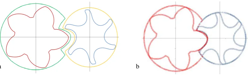
Kovačević (2002) [9] presented these aspects of grid generation in detail. Kovačević et al. (2002, 2005 and 2007) [9, 10, 11] have reported CFD simulations of twin screw machines to predict gas flow, conjugate heat transfer, fluid-structure interaction etc. for variety of screw machines. The domain of a screw machines is commonly decomposed into the low pressure port domain, the rotor domain and the high pressure port domain. A block structured numerical mesh is required in the stretching and sliding rotor domain in order to preserve conservativeness of the solution. The rotor grid is generated in the O form which requires a flow domain between rotors and the casing to be divided in two blocks each belonging to one of the rotors. One O grid is constructed on the side of the male rotor and other on the female side. The division is achieved by use of rack – the rotor with infinite radius which uniquely exists between two rotors. It is generated by use of envelope method of gearing as explained Kovačević et al. (2007) [11]. The rack and outer casing circles are connected in the cross section of the rotor domain to split it into two O grid domains as shown in Figure 1a. Boundary nodes are first positioned on the rotor boundaries using adaptation functions described in Kovačević (2005) [10] as shown in Figure 1b. These nodes retain relative position to the rotor and rotate together with the rotor. The boundary nodes on the outer boundary which consists of the casing circle and the rack are distributed using boundary distribution method described in Kovačević (2005) [10]. These nodes slide on the outer boundary as the rotor rotates. Such a grid is being referred to as Rotor to Casing grid or “RC grid”. In essence, each of the O grid block rotates and deforms. The two O grids used in this method slide relative to each other.

Rane et al. (2013 and 2014) [14, 15] recently extended the use of RC grid to generate deforming grids for variable geometry rotors with both variable lead and variable profile.

Figure 1 Decomposition of the rotor domain in algebraic rotor grid

a) O Grid boundaries, b) Discretised boundaries

4 The mentioned method for generating RC algebraic grids is fast and robust but introduces two grid features which require further attention namely, a non-conformal interface between the O grids and degenerated hexahedral numerical cells in the CUSP. Both of these are problematic for some CFD solvers as these cannot handle them conservatively. The objective of the work presented in this paper is to improve the grid generation method in order to resolve limitations caused by these undesired features of the RC type mesh.

1.1.1 Non-Conformal interface between blocks of RC grid.

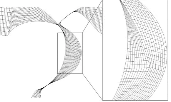
Figure 2 shows an example of a non-conformal interface between the two rotor blocks of a RC type grid. Such grids offer good quality cells in terms of orthogonality and aspect ratio which could be independently controlled by boundary distribution and adaptation as well as orthogonalisation and smoothing of the TFI grid as explained in Kovacevic et al (2007) [11]. But the presence of a non-conformal interface raises concerns about the conservativeness of the flux balance that will be achieved across the interface between two blocks and the stability of a solver in case of multiphase calculation with additional physical equations as in the case of liquid injection machines. Moreover not all solvers are capable of defining a robust interface with highly deforming, stretching and sliding interface as in a helical screw machines. The desired option is to generate a conformal interface in which the nodes will correspond in both domains or if possible to eliminate the interface completely and generate a single mesh block.

Figure 2 Non-conformal interface between the two rotors of RC type grid

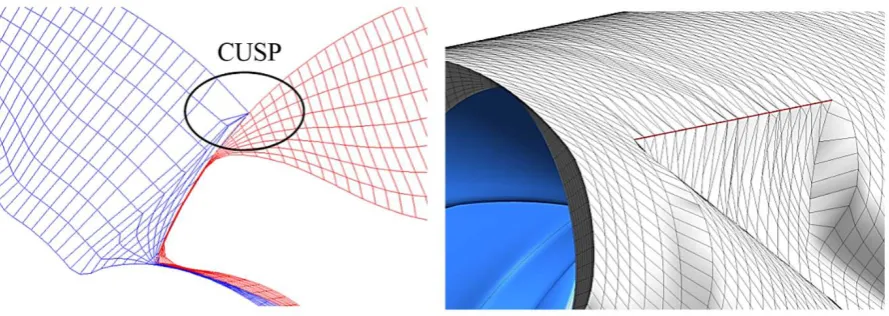
1.1.2 Degenerated hexahedral numerical cells in the CUSP

5 between the rotor bores in the axial direction which is required for accurate geometric representation of the blow-hole area, each numerical cell which slides on the casing boundary need to pass through the single point in the CUSP as shown in Figure 3. This is achieved by collapsing two neighbouring vertices of the boundary cell which results in creation of a cell with prism topology around the CUSP point. The cells still retain hexahedral definition with 8 vertices but some of these are simply occupying the same position in space. By this means the conservation of space is fully achieved but in some solvers, due to their internal node merging procedure, it results in degenerated numerical cells. Hence it is desirable to produce a grid with fully hexahedral cells which will retain all eight vertices to have different position in space during deformation.

Figure 3 Nodes merged at the CUSP point to capture blow-hole area in a RC type grid

1.2 Differential generation for twin screw rotor numerical grid

Fundamentals of differential grid generation are presented in many works such as Thompson, Thames and Mastin, (1974) [23], Soni, (1992) [20], Sorenson and Steger (1977 and 1979) [19 21], Shih et al. (1991) [18], Samareh and Smith, (1992) [17]. In the field of screw compressor rotor grids, Vande Voorde et al. (2004 and 2005) [25, 26] were the first to implement a grid generation algorithm for block structured mesh from the solution of the Laplace equation. In his thesis, Vande Voorde (2005) [27] presented the principles of solving the initial Laplace equation and then using it to construct a block structured deforming mesh from the equipotential and gradient lines as shown in Figure 4a. Based on this grid generation, flow in a double tooth compressor and a twin screw compressor was analysed.

6

Figure 4 Solution of Laplace equation – a) Iso-potential lines and b) Splitting curve

A numerical scheme can be used to solve the Laplace equation in the 2D domain so formed (Winslow, 1966 [28], Gordon and Hall, 1973 [6]). Since the rotor profiles have close tolerances, the region formed between the casing and the two profiles has a very complex boundary. The distance between the rotor and the casing can vary from a few millimetres in the core region to a few micrometres in the clearance regions. Hence, discretisation, using unstructured triangular cells is the most appropriate. The gaps can be highly refined to capture the iso-potential lines conforming with the boundary, accurately. Vande Voorde et al. (2005) [26] used a customised Delaunay triangulation program (Riemslagh et al., 2000) [16] for this initial triangular grid construction. In the final rotor grids, boundary nodes are first positioned on the casing and splitting curve. These nodes remain unchanged with respect to the rotor. The boundary nodes on the rotor are distributed with reference to the outer nodes. Rotor nodes slide on the profiles as the rotor rotates and cause warpage of the boundary cells on rotors with small radii in the profile as shown in Figure 5. Such a grid structure is referred to as Casing to Rotor grid type or in short CR type grid.

Figure 5 Warpage of faces at small radii on the two rotors of CR type grid

7

1.3 Comparison of the algebraic method RC grid and differential CR grid

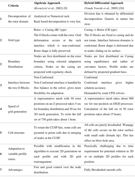
Table 1 shows comparison of the grid generation methods used for analysis for screw machines. It is based on the features of the RC type grid generated using algebraic method from Kovačević et al. (2002) [9] and the CR type grid using hybrid differential method from Vande Voorde et al. (2005) [26].

Table 1 Comparison of algebraic and differential grid generation in twin screw compressors

Criteria Algebraic Approach

(Kovačević et al., 2002) [9]

Hybrid Differential Approach

(Vande Voorde et al., 2005) [26]

1 Decomposition of

the rotor domain

Analytical or Numerical rack.

Rack based decomposition is very fast.

Division line is obtained by differential

decomposition. Generic in nature but

slow.

2 Grid type

Rotor ⇒ Casing (RC type)

The O blocks rotate with the rotor. Grid

deformation occurs at the rack

interface which is non-conformal.

Rotor shape is fully preserved.

Casing ⇒ Rotor (CR type)

The O blocks are fixed to casing and do

not rotate. Interface between domains is

conformal. Rotor shape is deformed due

to nodes sliding on its surface.

2 Boundary

Distribution

Nodes are first distributed on the rotor

boundary using selected adaptation

criteria. Nodes on the casing are

projected with regularity check.

Nodes are first distributed on Casing

using equidistance and radius of

curvature factors. Profile nodes are

defined by projected gradient lines.

3 Interface between

the two O Blocks

Non-Conformal.

Non-Conformal interface is handled by

flux balance in the solver, gives more

flexibility for adaptation.

Conformal.

Conformal interface gives higher

solution accuracy.

Demanded by some CFD solvers.

4 Speed of

grid generation

A representative mesh with 50 rotor

positions on an i3 processor takes 5 sec

for boundary distribution and 30 sec for

2D mesh generation. To write the full

set of 750 grids takes about 1 hour.

A representative mesh takes about 900

sec for one position on DS20 processor.

Calculation of the full set of 50 rotor

positions takes about 15 hours.

5 Cell structure

To retain the CUSP line, some cells are

pyramid or prism cells due to merging

of nodes at the CUSP.

All cells are purely hexahedral. Warpage

of the cells occurs on the rotor surface

with small radii (female tip). This has

effect on blow-hole area.

6

Adaptation to

variable profile

rotors

Possible with modification in the

algorithm to execute 2D generation on

each profile and with 3D grid

rearrangement.

Practically challenging due to time

requirement for potential solution in 3D

or on multiple 2D profiles for each

position.

7 Advantages Fast and good control over the node

8

Rotor profile smoothly captured grid.

Grid refinement is easy to be achieved.

Conformal interface between O blocks

makes the grid suitable for variety of

solvers and complexities like Multiphase

flows.

8 Difficulties

Some solvers cannot handle

non-conformal interface between the

domains.

Computationally expensive and long

grid generation procedure. Difficulty of

handling profiles with very small radii in

the profile shape.

As identified in Table 1, the differential method proposed by Vande Voorde et al. (2005) [26] has some advantages compared to algebraic method developed by authors. These are mainly due to the use of iso-potential lines to produce the mesh with fixed nodes on the casing and conformal interface between the O grids.

The objective of the work described in this paper is to develop an algebraic grid generation method for a single domain grid which will combine advantages of both algebraic methods speed and CR mesh convenience.

2

Algebraic generation for single domain grid of screw machines

By using a CR type grid it is possible to generate fully hexahedral cells and conformal interface between the O blocks by using algebraic method and achieve similar characteristics of the grid obtained by the differential approach but in much shorter time. However, the CR distribution using algebraic methods does not give reference to distribution of boundary points on rotors which was available in the differential approach through the iso-potential solution. Therefore, it is challenging to achieve a regular grid on rotors without any special treatments.

9

2.1 Coordinate transformations for generation of CR type grid

The main steps in generating the CR type grid are:

1. Split the rotor cross section into two O blocks using rack as the splitting curve (Figure 1a). 2. Define the outer boundary in each O block as a combination of the casing circle between the

CUSPs around the rotor and rack between the rotors as shown in Figure 6. 3. Discretize the Casing part of the outer boundary using equidistant distribution.

4. Discretise the rack part of the outer boundary so that the same number of nodes is selected for both O blocks in order to maintain a conformal interface. This distribution does not need to be equidistant and could also be adapted based on the characteristics of rotor curves in the interlobe region. Figure 6 shows the distribution obtained on the outer boundaries of the two O blocks that will act as the reference for the rotor profile distribution.

5. Define inner boundary by the original points of the rotor profile.

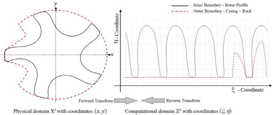
6. Make coordinate transformation of the outer boundary and the inner boundary from the physical domain X2 with coordinates (𝑥𝑥,𝑦𝑦) to the computational domain Ξ2 with coordinates (ξ,η) as shown in Figure 7 and defined by equations 2 and 3.

7. Distribute nodes on the rotor profile with corresponding distribution available on the outer boundary. The initial distribution can be selected as the constantξ coordinate intersections with the transformed rotor profile to get theη coordinate. But this will produce overlap in some regions, especially on the gate rotor as shown in Figure 8. This requires for this distribution to be regularised.

8. Regularise the rotor profile distribution. Two methods of regularisation have been presented in this paper and described in sections 2.2 and 2.3.

• Analytical control function.

• Background blocking distribution.

9. Reverse coordinate transformation from (ξ,η) to (𝑥𝑥,𝑦𝑦) domain to get the rotor geometry as defined by equation 5.

10. Produce numerical mesh using TFI (Kovačević et al., 2002 [9], Eiseman et al. 1994 [3], Kim and Thompson, 1990 [7]).

10

Figure 6 CR type grid point distribution of inner boundary and outer circle

Figure 7 Physical and Computational domains with coordinate transformation of inner and outer boundary

The more detailed description of steps 3, 4, 5, 6 and 7 is given below.

A mapping function is used to transform the full inner and outer boundary from the physical to the computational domain. In the case of the RC type grid, this transformation needs to be performed only for one interlobe space since the distribution of the inner boundary remains unchanged for the entire rotor. However, for the CR type grid, each interlobe may have a different number of nodes and their distribution on the rotor profile may change. Therefore, it is necessary to make a coordinate transformation for the full profile span.

11 on the outer boundary are 𝒓𝒓_{𝑖𝑖,𝑗𝑗=1}(𝑥𝑥,𝑦𝑦). In addition, an outer circle with diameter larger than the rotor outer diameter is discretised using the nomenclature 𝒓𝒓_{𝑖𝑖,𝑗𝑗}′₌₁(𝑥𝑥,𝑦𝑦), as shown in Figure 6.

The node distribution starts at the bottom CUSP which has index i=0. Based on the equidistant spacing, the distribution of the outer boundary is defined as,

�𝒓𝒓𝑖𝑖,𝑗𝑗=1(𝑥𝑥,𝑦𝑦)�=�𝒓𝒓𝑖𝑖−1,𝑗𝑗=1(𝑥𝑥,𝑦𝑦)�+ 𝑆𝑆𝑖𝑖𝑖𝑖 (1)

𝑆𝑆𝑖𝑖 =𝑆𝑆_II is the increment in spacing per node. 𝑆𝑆𝐼𝐼is the length of the boundary and I is the number of

nodes on the rack and casing which can be set independently. The transformation from the physical regionΧ2 onto a computational domainΞ2is such that the outer circular boundary becomes a straight line along theξcoordinate. The transformation is described by equations (2a, 2b and 2c) below. It is to be noted that in the forward transformation, the rotor profile is defined with a high density array while in the reverse transform, the inner boundary is discretised with the same number of points as the outer boundary.

Outer boundary

ξ_{𝑖𝑖,𝑗𝑗=1}(𝑥𝑥,𝑦𝑦) = tan−1_�𝑦𝑦𝑖𝑖,𝑗𝑗=1

𝑥𝑥𝑖𝑖,𝑗𝑗=1�

η_{𝑖𝑖,𝑗𝑗=1(𝑥𝑥,𝑦𝑦) =𝑟𝑟𝑜𝑜− �𝑥𝑥𝑖𝑖,𝑗𝑗=1}2_{+𝑦𝑦𝑖𝑖,𝑗𝑗=1}2

(2a)

Outer circle

ξ_{𝑖𝑖,𝑗𝑗}′₌₁(𝑥𝑥,𝑦𝑦) = tan−1�𝑦𝑦𝑖𝑖,𝑗𝑗 ′₌₁

𝑥𝑥𝑖𝑖,𝑗𝑗′₌₁�

η_{𝑖𝑖,𝑗𝑗}′₌₁(𝑥𝑥,𝑦𝑦) =𝑟𝑟_𝑜𝑜− 𝑟𝑟_{𝑜𝑜𝑐𝑐}

(2b)

Inner boundary

ξ_{𝑖𝑖,𝑗𝑗=0(𝑥𝑥,𝑦𝑦) = tan}−1_�𝑦𝑦𝑖𝑖,𝑗𝑗=0

𝑥𝑥𝑖𝑖,𝑗𝑗=0�

η_{𝑖𝑖,𝑗𝑗=0(𝑥𝑥,𝑦𝑦) =𝑟𝑟𝑜𝑜− �𝑥𝑥𝑖𝑖,𝑗𝑗=0}2_{+𝑦𝑦𝑖𝑖,𝑗𝑗=0}2

(2c)

Where, 𝑟𝑟𝑜𝑜 is the radius of the rotor and 𝑟𝑟𝑜𝑜𝑐𝑐 is radius of outer circle.

The reverse transformation from computational domain to physical region is required only for the rotor profile in order to obtain the distribution of the inner boundary nodes on the rotor in the physical domain. This reverse transformation is represented by the following equation (3).

12 𝑦𝑦𝑖𝑖,𝑗𝑗=0(ξ,η) =𝑎𝑎𝑎𝑎𝑎𝑎 �𝑟𝑟0−η𝑖𝑖,𝑗𝑗=0(𝑥𝑥,𝑦𝑦)� 𝑎𝑎𝑖𝑖𝑛𝑛 �ξ𝑖𝑖,𝑗𝑗=0(𝑥𝑥,𝑦𝑦)�

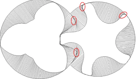
Figure 8 shows the distribution obtained after the reverse transformation. Here the distribution on the inner boundary is obtained using equidistant distribution.

Figure 8 Reverse transformation of full rotor region to physical domain

As shown in Figure 8, the difference in rotor curvatures may result in a significant number of irregularities and crossing of the distribution lines. However, at the same time a conformal interface has been achieved between the two O blocks which renders the need for merging nodes on the CUSP point. This is because grid points on the outer boundary are stationary and both CUSPs have the same index i

in all the cross sections forming naturally a straight CUSP line. However it is necessary to regularise the distribution on the inner boundary in the computational domain before the reverse transformation is carried out in order to ensure that the final distribution of the nodes on the rotor surface is regular.

2.2 Regularisation approach using analytical control function

13 outer circle and also control the location of the focus point to which these points will attract or repel. Such a control is achieved by a skewed sine function defined in equation 4.

𝑓𝑓(𝑡𝑡) =𝐴𝐴𝑠𝑠𝑠𝑠− 𝑎𝑎𝑎𝑎𝑎𝑎 �𝐴𝐴𝑠𝑠𝑠𝑠 sin�2 𝜋𝜋𝑛𝑛𝑠𝑠𝑠𝑠 _𝑡𝑡𝑡𝑡

𝑖𝑖− 𝜎𝜎𝑠𝑠𝑠𝑠𝑎𝑎𝑎𝑎𝑎𝑎 �sin �2 𝜋𝜋𝑛𝑛𝑠𝑠𝑠𝑠

𝑡𝑡

𝑡𝑡𝑖𝑖���� (4)

Points are represented by the index i. Skewness value controls the location where the function will have zero value while the amplitude controls the magnitude of the function at a given point. The number of cycles of the function correspond to the number of lobes on the rotor.

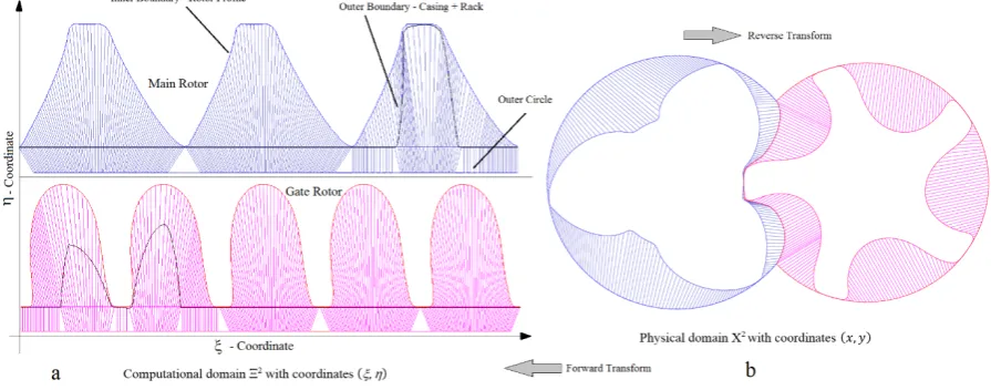
Figure 9a shows the regularised distribution obtained on the main and gate rotors in the computational space. In the interlobe space where the outer boundary is represented by the rack curve, the sine function is made to work only between the CUSP points. The casing points on the outer boundary are aligned with the starting and ending points in two CUSPs to provide smooth distribution. Figure 9b shows the distribution in the physical domain obtained by reverse transformation where the required properties of the conformal interface are achieved in each 2D cross section using the skewed sine function.

Figure 9 CR distribution obtained with skewed sine function – a) Computational space, b) Physical space

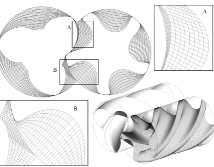
An example of the CR mesh with the conformal interface produced using skewed sine adaptation of the rotor distribution is shown in Figure 10 on “N” profile rotors with 3 male rotor lobes and the gate rotor of 5 lobes. These rotors have deep lobes with small radii at the rotor tip and the convex trailing side of the female rotor lobe. Because of these features a relatively high skewness and amplitude factors are required to achieve regular distribution in 2D cross sections. Figure 10 shows details of the cross section with the interface regions and the 3D grid of the helical rotors.

14 distribution (Figure 8). Final values reported in Table 2 were obtained by gradual increment such that distribution becomes regular (Figure 9b). Cell quality has not been considered at this stage.

Table 2 Control parameters for sample case using skewed sine function

Total number of circumferential nodes 250 Circumferential nodes in the interlobe 65

Radial Nodes 8

Angular divisions per interlobe angle 50

Skewed sine function: Main Rotor Skewness +0.2 Amplitude 0.25 Gate Rotor Skewness −0.5 Amplitude 0.24

However, generation of a 3D mesh showed highly skewed cells on the surface of the male rotor occurring in the place of an abrupt change in the rack curve shape between two consecutive cross sections, as shown in Figure 11. This difficulty was not observed for the rotors with straight lobes because all cross sections in such rotors are identical but a jump in the cell shape was noticed. As such, the method of using a skewed sine function for regularisation of rotor profile distribution has been successful for generation of conformal fully hexahedral grids for rotors with straight lobes, but was not successful for screw rotors with helical lobes.

Figure 10 Conformal grid regularised by use

of skewed sine function

Figure 11 Degenerated faces on the rotor surface in

3D grids

2.3 Regularisation approach using background blocking technique

15 1999 [24], Eiseman et al., 1994 [3]). The procedure is used to distribute nodes on the inner boundary (rotors) of the new CR type mesh by use of background blocks generated from the RC type grid. Apart of regularisation of distribution, this approach can be used for an independent refinement of the grid in the interlobe region in order to improve the mesh quality in the interlobe leakage gaps.

A skewed sine function for regularisation of the rotor profile distribution independently regularised each 2D cross section. This produced degenerated cells in the 3D mesh. In order to achieve regular 3D mesh with helical rotors, distribution on the rotor profile requires reference to adjacent cross sections. The distribution of points on the rotor surface in RC grid type, which is directed from the rotor profile to the outer boundary generates a very good quality rotor surface mesh. This feature of the RC grid type makes this distribution suitable for background blocking in the new CR type distribution on the rotor profile.

2.3.1 Generating background blocks

Background blocks are produced by equidistant distribution in the RC grid type on the outer computational circle. The outer circle will normally have diameter of the rotor bores as shown in Figure 12.

Background blocks are generated using following steps:

1. Nodes on the rotor profile in each interlobe are distributed, using equidistant distribution. If required adaptation described in (Kovačević et al., 2002) [9] can be applied.

2. The distribution on the outer circle is based on regularised arc-length as described in Kovačević

et al., 2002 [9].

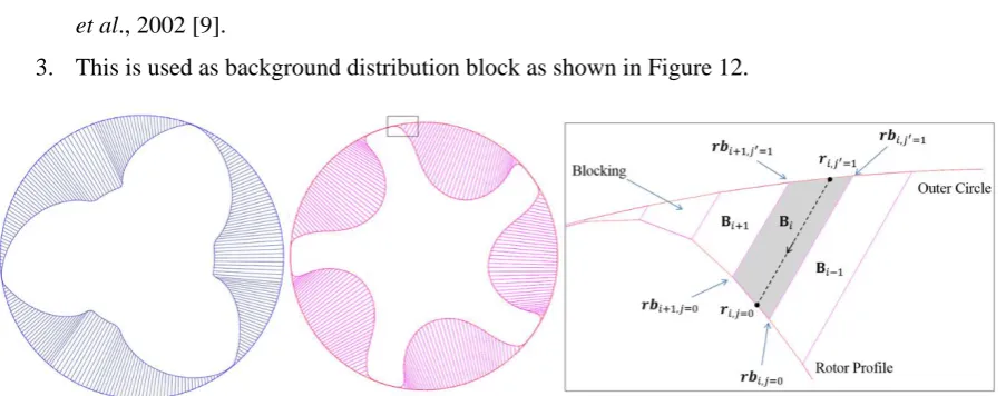
3. This is used as background distribution block as shown in Figure 12.

Figure 12 Background blocking for the main and gate rotors and projection function

The advantages of generating such blocks are:

˗ The blocks do not have to be as refined as the final grid.

˗ The blocks can be used as reference for refinement in any required region.

16

2.3.2 Application of background blocking

As shown in Figure 6 the points distributed on boundaries are represented in the index notation with respect to the physical coordinate system as 𝒓𝒓_{𝑖𝑖,𝑗𝑗}(𝑥𝑥,𝑦𝑦). Points on the inner boundary (rotor profile) are𝒓𝒓_{𝑖𝑖,𝑗𝑗=0}(𝑥𝑥,𝑦𝑦), points on the outer boundary which consists of casing and rack curve are𝒓𝒓_{𝑖𝑖,𝑗𝑗=1}(𝑥𝑥,𝑦𝑦) and the points distributed on the outer circle are 𝒓𝒓_{𝑖𝑖,𝑗𝑗}′₌₁(𝑥𝑥,𝑦𝑦).

Each of the background blocks is identified by its index𝐁𝐁_𝑖𝑖. The background block points on the inner boundary of the blocks are𝒓𝒓𝒓𝒓_{𝑖𝑖,𝑗𝑗=0}(𝑥𝑥,𝑦𝑦) and the background block points on the outer full circle are𝒓𝒓𝒓𝒓_{𝑖𝑖,𝑗𝑗}′₌₁(𝑥𝑥,𝑦𝑦) as shown in Figure 12.

Starting from the bottom CUSP, nodes are distributed on the outer circle corresponding to the rack part with required number of points𝑖𝑖_{𝑟𝑟𝑐𝑐𝑐𝑐𝑠𝑠}as shown in Figure 13. The remaining nodes are distributed on the outer circle covering the casing part with required number of points𝑖𝑖_{𝑐𝑐𝑐𝑐𝑠𝑠𝑖𝑖𝑐𝑐𝑐𝑐}. Factors𝑖𝑖_{𝑟𝑟𝑐𝑐𝑐𝑐𝑠𝑠}and 𝑖𝑖_{𝑐𝑐𝑐𝑐𝑠𝑠𝑖𝑖𝑐𝑐𝑐𝑐} can be independently selected for the main and the gate rotor or they can be set such that the sum

𝑖𝑖𝑟𝑟𝑐𝑐𝑐𝑐𝑠𝑠+𝑖𝑖𝑐𝑐𝑐𝑐𝑠𝑠𝑖𝑖𝑐𝑐𝑐𝑐 is maintained. Increasing the number of points in the interlobe between two CUSPS

𝑖𝑖𝑟𝑟𝑐𝑐𝑐𝑐𝑠𝑠 will coarsen the casing part and refine the rack part of the outer boundary. At this stage

𝒓𝒓𝒓𝒓𝑖𝑖,𝑗𝑗=0(𝑥𝑥,𝑦𝑦), 𝒓𝒓𝒓𝒓𝑖𝑖,𝑗𝑗′₌₁(𝑥𝑥,𝑦𝑦) 𝑎𝑎𝑛𝑛𝑎𝑎 𝒓𝒓_{𝑖𝑖,𝑗𝑗}′₌₁(𝑥𝑥,𝑦𝑦) are known and it is required to calculate the position of the new point on the rotor 𝒓𝒓_{𝑖𝑖,𝑗𝑗=0}(𝑥𝑥,𝑦𝑦) as shown in Figure 12. This node distribution is based on equidistant spacing

�𝒓𝒓𝑖𝑖,𝑗𝑗′₌₁(𝑥𝑥,𝑦𝑦)�=�𝒓𝒓_{𝑖𝑖−1,𝑗𝑗}′₌₁(𝑥𝑥,𝑦𝑦)�+ 𝑆𝑆_𝑖𝑖𝑖𝑖 (5)

where𝑆𝑆_𝑖𝑖 =𝑆𝑆I

I ,𝑆𝑆𝐼𝐼 =𝒓𝒓𝐼𝐼,𝑗𝑗′=1(𝑥𝑥,𝑦𝑦)− 𝒓𝒓𝑖𝑖=0,𝑗𝑗′=1(𝑥𝑥,𝑦𝑦). Since the calculation of new point using equation

(5) is separate for the rack part and for the casing part, value of I = 𝑖𝑖_{𝑟𝑟𝑐𝑐𝑐𝑐𝑠𝑠} on the rack and I = 𝑖𝑖_{𝑐𝑐𝑐𝑐𝑠𝑠𝑖𝑖𝑐𝑐𝑐𝑐} on the casing. The process is managed by a scanning function which has the information of the background blocking. Starting from the bottom CUSP, the scanning function traces each node𝒓𝒓_{𝑖𝑖,𝑗𝑗}′₌₁(𝑥𝑥,𝑦𝑦) and identifies the block𝐁𝐁_𝑖𝑖 to which this node belongs. There can be a situation when a single block contains multiple nodes of the distribution on the outer boundary or blocks which contain no nodes. This is because the distribution on the outer boundary can be refined either in the rack part or in the casing part and be different than the blocking. Once the nodes associated with each block are found by the scanning function, an arc-length based projection is used to determine the nodes𝒓𝒓_{𝑖𝑖,𝑗𝑗=0}(𝑥𝑥,𝑦𝑦) to be placed on the inner boundary - rotor profile. At the same time constraint is imposed on the node placement that they have to be bound in the same block𝐁𝐁_𝑖𝑖 as that of the outer circle nodes𝒓𝒓_{𝑖𝑖,𝑗𝑗}′₌₁(𝑥𝑥,𝑦𝑦).

17 𝒓𝒓𝑖𝑖,𝑗𝑗=0(𝑥𝑥,𝑦𝑦) =𝒓𝒓𝒓𝒓𝑖𝑖,𝑗𝑗=0(𝑥𝑥,𝑦𝑦) +�𝒓𝒓𝒓𝒓𝑖𝑖+1,𝑗𝑗=0(𝑥𝑥,𝑦𝑦)− 𝒓𝒓𝒓𝒓𝑖𝑖,𝑗𝑗=0(𝑥𝑥,𝑦𝑦)� 𝑆𝑆_𝑆𝑆𝑖𝑖

𝐼𝐼

𝑆𝑆𝑖𝑖 = 𝒓𝒓𝑖𝑖,𝑗𝑗′=1(𝑥𝑥,𝑦𝑦)− 𝒓𝒓𝒓𝒓𝑖𝑖,𝑗𝑗′=1(𝑥𝑥,𝑦𝑦)

𝑆𝑆𝐼𝐼 =𝒓𝒓𝒓𝒓𝑖𝑖+1,𝑗𝑗′₌₁(𝑥𝑥,𝑦𝑦)− 𝒓𝒓𝒓𝒓_{𝑖𝑖,𝑗𝑗}′₌₁(𝑥𝑥,𝑦𝑦)

(6)

The calculated position of inner boundary nodes 𝒓𝒓_{𝑖𝑖,𝑗𝑗=0}(𝑥𝑥,𝑦𝑦) ensure that they are placed on the original rotor profile. Regularised distribution is then superimposed onto the outer boundary - rack curve by finding the intersection points of the distribution line and the rack curve. These intersection points define the new point distribution𝒓𝒓_{𝑖𝑖,𝑗𝑗=1}(𝑥𝑥,𝑦𝑦) on the rack curve as shown in Figure 13.

Figure 13 Refinement in the rack segment and superimposition of rack curve

The blocks are different on the male and the female rotor side and accordingly the intersection points obtained on the common rack on the two O blocks are initially different. This results in a non-conformal interface between the two rotor blocks but gives the grid an important capability of refinement in the interlobe region. This flow region contains interlobe gaps which are a big factor in the performance of the machine and therefore accurate capturing of the rotor profile in the leakage gaps has a strong influence on the solution of the leakage flow calculation.

Additionally, it is possible to constrain the node distribution on the rack segment of the outer boundary to be same for both O blocks of the main and gate rotor and therefore achieve a one to one conformal interface as shown in Figure 14. Thus a non-conformal interface can be replaced by the conformal interface and a single domain structure for the rotor mesh can be constructed.

2.3.3 Regularised grid with background blocking

18

Table 3 Grid parameters for sample case using background blocking.

Blocks per interlobe Main Rotor 80 Gate Rotor 50 Total number of circumferential nodes 250 Circumferential nodes in the interlobe 75

Radial Nodes 8

Angular divisions per interlobe angle 50

19

Figure 14 Grid generated with background blocking in

screw compressor rotor

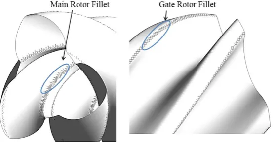
Figure 15 Surface mesh on the rotor, casing and the

rack interface

The CR grid type is characterised by the stationary casing mesh and sliding mesh on the rotors. Due to this sliding action some face warping of the cells are noticeable at the root of the main rotor and at the tip of the gate rotor where normally small fillets are introduced in the rotor profile, as shown in Figure 15. This is reported also in Vande Voorde (2005) [27] and is a feature of CR type grid which does not happen in the RC grid type where the nodes rotate together with rotors. The effect of this face warping can be reduced by increasing number of points on the grid and is assessed further in the section 3 of this paper.

2.4 Examples

The examples of interlobe refinement and the conformal interface between the blocks are shown here to demonstrate capability of the new method for generating single domain numerical mesh for screw machines.

2.4.1 Example of the grid with interlobe refinement

Figure 16 shows an example of successively increased refinement in the interlobe region. The sum of 𝑖𝑖𝑟𝑟𝑐𝑐𝑐𝑐𝑠𝑠+𝑖𝑖𝑐𝑐𝑐𝑐𝑠𝑠𝑖𝑖𝑐𝑐𝑐𝑐 is maintained constant while the number of points on the rack are increased. This has

20

Figure 16 Examples of grids with interlobe refinement

2.4.2 Example of the grid with conformal interface

Figure 17 shows an example of the grid in cross section with the conformal interface between the two O blocks which features node to node connection. The distribution was generated first on the rack part of the gate rotor and maintained identical on the main rotor block thus achieving a conformal interface the interlobe region.

21 In the process of generating a 3D mesh for solving the fluid flow around these rotors, the corresponding nodes in the interface are collapsed in the single node and a single domain cell structure is produced.

3

Evaluation of the cell quality of the CR type grids

Numerical grids used for calculation of fluid flow by Computational Fluid Dynamics (CFD) need to be acceptable by the flow solver, have all cells regular and should capture the geometry at boundaries as accurately as possible. If a large numbers of cells are with poor quality then the error induced in numerical calculations is large resulting in inaccurate or false predictions from the CFD models. At the same time large number of poor quality cells can lead to solver instability and convergence issues particularly at higher operating pressure ratio. Moreover, even if the calculation is possible, large number of poor quality cells will increase calculation time to achieve desired convergence criteria. Some of the important quality criteria for finite volume numerical methods are orthogonality, skewness, aspect ratio and warpage of cells. These are considered below for evaluation of the CR type grids. For comparison, two grid types are considered, as follows:

Grid A – RC grid type which has been well validated as acceptable for flow solutions using variety of CFD solvers including ANSYS CFX solver (Kovačević et al., 2007) [11].

Grid B – the newly formulated algebraic CR grid type produced by background blocking regularization. The size of the mesh in terms of the node count and spacing in the circumferential, radial and axial directions is same for both grids. The commercial ICEM CFD tool from ANSYS has been used for the calculation of quality factors and plotting of selected cells.

3.1 Orthogonality

The orthogonality is a cell quality defined as the cosine of the angle between the vector normal to the cell face and the vector from the cell centroid to the centroid of the adjacent cell or the vector from the cell centroid to its face centroid. The smaller of the two values is selected. A value of 1 represents a perfect hexahedral cube and a value of 0 is a fully degenerated hexahedron.

22

Figure 18 Comparison of Grid A and Grid B - % cells vs Quality factor

3.2 Equiangular Skewness

Equiangular Skewness is calculated as the deviation of the cell with respect to a perfect cubic hexahedron as given by equation (7). A value of 1 represents a perfect hexahedral cube while a value of 0 represents a fully degenerated hexahedron.

𝐸𝐸𝐸𝐸𝐸𝐸𝑖𝑖𝑎𝑎𝑛𝑛𝐸𝐸𝐸𝐸𝐸𝐸𝑎𝑎𝑟𝑟𝑆𝑆𝑆𝑆𝑆𝑆𝑆𝑆𝑛𝑛𝑆𝑆𝑎𝑎𝑎𝑎= 1.0− 𝑀𝑀𝑎𝑎𝑥𝑥 �(₍₁₈₀𝑄𝑄𝑚𝑚𝑐𝑐𝑚𝑚_{− 𝑄𝑄}− 𝑄𝑄𝑒𝑒)

𝑒𝑒) ,

(𝑄𝑄𝑒𝑒− 𝑄𝑄𝑚𝑚𝑖𝑖𝑐𝑐)

𝑄𝑄𝑒𝑒 �

Where, 𝑄𝑄_{𝑚𝑚𝑐𝑐𝑚𝑚}𝑎𝑎𝑛𝑛𝑎𝑎𝑄𝑄_{𝑚𝑚𝑖𝑖𝑐𝑐}= largest and smallest angle in the element

𝑄𝑄𝑒𝑒= 90°, angle of an equiangular element

(7)

Figure 19 Comparison of cells with Equiangular Skewness factor < 0.15

23 cells with equiangular skewness lower than 0.15 while Grid B has about 0.35% cells with equiangular skewness lower than 0.15. The location of cells with the equiangular skewness < 0.15 is shown graphically in Figure 19. The Grid B of CR type shows great improvement in skewness compared to the original mesh. The highest degeneration of cells is on the interface in the interlobe region which indicates that it may be possible to improve this further by smoothing the interface curve.

3.3 Aspect Ratio

The Aspect Ratio is an indicator of the degree of stretching on the cells. For an individual hexahedral cell it is defined as the ratio of its maximum face area to its minimum face area. For the entire grid the largest ratio is considered as the maximum aspect ratio. In Grid A the aspect ratio was found to be 230 in the main rotor and 280 in the gate rotor in less than 0.1% cells. In Grid B the aspect ratio was found to be 443 in the main rotor and 348 in the gate rotor in less than 0.1% cells. Maximum Aspect ratio recommended by ANSYS CFX solver is less than 100. But for double precision it can be as high as 1000 in limited number of cells. Cell locations with aspect ratio exceeding 200 are represented graphically in Figure 20 which clearly shows that these high aspect ratio cells are present in the radial and interlobe leakage gaps.

Figure 20 Comparison of regions with aspect ratio > 200

3.4 Face warp angle

24 of the cells as compared with those in Grid A. In Grid A, 96% of cells have a good Warp angle in the range of 0° – 10° while in Grid B this number has reduced to 75%.

Figure 21 Comparison of cells with MaxWarp factor > 50

From the analysis of above quality parameters it can be concluded that the CR grid type have acceptable quality for the solver. The cell orthogonality and equiangular skewness have improved significantly, but the maximum warp angle has increased for the CR type grid when compared to RC type grid. The aspect ratio was maintained in the same range in both grid types.

4

Conclusions

Computational fluid dynamics of twin screw machines requires special attention in the generation of a computational grid that needs to represent the highly deforming working chamber in such machines. In practise two algorithms are available namely, an algebraic decomposition method from Kovačević et al (2002) [9] and a differential decomposition method from Vande Voorde et al (2005) [26]. Algebraic methods produce RC type mesh which rotates with rotors and take very little time measured in minutes to produce full mesh while the differential methods produce CR type mesh which is stationary on the casing and slides on the rotors and take very long time measured in tens of hours to obtain converged mesh. In this paper an algebraic method is developed in order to improve speed and accuracy of the CFD solution and enable use of variety of CFD solvers for analysis of screw machines. A new algebraic boundary distribution of CR type has been implemented to generate a single domain rotor grid. This paper presented the implementation and grid characteristics of the new method.

• Using a boundary distribution governed from the casing boundary to the rotor boundary (CR type grids) and the regularisation functions, it was possible to achieve desirable characteristics in the twin screw rotor domain;

25 ˗ Secondly, a highly significant achievement is a single domain structured grid for the rotors which eliminates a non-conformal interface between the two rotor domains, while still maintaining the fully hexahedral cell topology.

• Regularisation based on analytical function was suitable for non-helical rotors but failed for helical screw rotors due to degeneration of the rotor surface mesh.

• Regularisation based on background blocking approach was highly successful, easy to implement and robust.

• The speed of calculation of the numerical mesh is very short allowing the full moderate size mesh of around 1 million cells to be generated within few minutes in comparison with differential methods which use more than 10 hours to generate similar mesh.

• With this CR grid approach, an improvement in the global orthogonality and skewness of the cells was measured in a 3/5 helical screw rotor mesh.

• Aspect ratio did not show a significant difference between the RC type and CR type grid structures.

• With CR type structure, there was a decrement in the face warp quality at tip of the rotors which will need attention in further work.

This development allowed the use of numerical mesh generated by algebraic grid generation with variety of CFD solvers including popular ones like ANSYS CFX, ANSYS Fluent, CD Adapco STAR-CCM+ and Simerics PD.

References

[1] Chawner J. R., Anderson D. A., 1991. Development of an Algebraic Grid Generation Method with Orthogonality and Clustering Control, Conference on Numerical Grid Generation in CFD and Related Fields at Barcelona, 107.

[2] Eiseman P. R., 1987. Adaptive grid generation. Comput. Methods. Appl. Mech. Eng. 64, 321-376.

[3] Eiseman P.R., Hauser J., Thompson J.F., Weatherill N.P., (Ed.), 1994. Numerical Grid Generation in Computational Field Simulation and Related Fields, Proceedings of the 4th International Conference, Pineridge Press, Swansea, Wales, UK.

[4] Farrashkhalvat M., Miles P. J., 2003. Basic structured grid generation with an introduction to unstructured grid generation. BH publication Oxford. ISBN 0 7506 5058 3.

[5] Ferziger J. H. and Perić M., 1996. Computational Methods for Fluid Dynamics, ISBN 978-3-540-42074-3, Springer, Berlin, Germany.

26 [7] Kim J. H., Thompson J.F, 1990. 3-Dimensional Adaptive Grid generation on a

Composite-Bloch Grid, AIAA Journal, Vol.28, Part.3, 470-477.

[8] Kovačević A., Stošić N., Smith I. K., 2000. Grid Aspects of Screw Compressor Flow Calculations, ASME Congress, Orlando FL, Vol. 40, pp. 83.

[9] Kovačević A., 2002. Three-Dimensional Numerical Analysis for Flow Prediction in Positive Displacement Screw Machines, Ph.D. Thesis, School of Engineering and Mathematical Sciences, City University London.

[10] Kovačević A., 2005. Boundary Adaptation in Grid Generation for CFD Analysis of Screw Compressors, Int. J. Numer. Methods Eng., Vol. 64: 401-426.

[11] Kovačević A., Stošić N. and Smith I. K., 2007. Screw compressors - Three dimensional computational fluid dynamics and solid fluid interaction, ISBN 3-540-36302-5, Springer-Verlag Berlin Heidelberg New York.

[12] Kovačević A. and Rane S., 2013. 3D CFD analysis of a twin screw expander, 8th International conference on compressors and their systems, London, p. 417.

[13] Papes, I., Degroote, J., Vierendeels, J., 2014. 3D CFD analysis of a twin screw expander for small scale ORC systems. Proceedings of the 11th World Congress on Computational Mechanics. pp. 7207–7217.

[14] Rane S., Kovačević A., Stošić N. and Kethidi M., 2013. Grid Deformation Strategies for CFD Analysis of Screw Compressors, Int Journal of Refrigeration, 36, 7, p. 1883-1893. [15] Rane S., Kovačević A., Stošić N. and Kethidi M., 2014. Deforming grid generation and

CFD analysis of variable geometry screw compressors, Computers and Fluids, 99, p. 124–141. [16] Riemslagh K., Vierendeels J., Dick E., 2000. An arbitrary Lagrangian-Eulerian

finite-volume method for the simulation of rotary displacement pump flow. Applied Numerical Mathematics, 32:419-433.

[17] Samareh A. J., Smith R.E., 1992. A Practical Approach to Algebraic Grid Adaptation, Computers Mathematical Applications, Vol.24, No.5/6, 69-81.

[18] Shih T. I. P., Bailey R. T., Ngoyen H. L., Roelke R. J., 1991. Algebraic Grid Generation for Complex Geometries, International Journal for Numerical Methods in Fluids, Vol. 13, 1-31.

[19] Sorenson R. L., Steger J. L., 1977. Simplified clustering of nonorthogonal grids generated by elliptic partial differential equations. Ames research centre, Moffett field, California, NASA Technical Memorandum 73252.

[20] Soni B.K, 1992. Grid Generation for Internal Flow Configurations, Computers Mathematical Applications, Vol.24, No.5/6, 191-201.

27 [22] Stošić N, Smith I.K, Zagorac S, 1996. CFD Studies of Flow in Screw and Scroll

Compressors. Proc. Int. Compressor Conf. at Purdue. Paper 1103.

[23] Thompson J. F., Thames F. C., Mastin C. W., 1974. Automatic Numerical Generation of Body-Fitted curvilinear coordinate system for field containing any number of arbitrary two-dimensional bodies. J. Comput. Phys., vol. 15, pp. 299-319.

[24] Thompson J. F, Soni B and Weatherill N. P, 1999. Handbook of Grid Generation, CRC Press.

[25] Vande Voorde J., Vierendeels J., Dick E., 2004. A Grid Generator for flow calculations in Rotary Volumetric Compressors, European Congress on Computational Methods in Applied Sciences and Engineering.

[26] Vande Voorde J., Vierendeels J., 2005. A grid manipulation algorithm for ALE calculations in screw compressors. 17th AIAA Computational Fluid Dynamics Conference, Canada, AIAA 2005-4701.

[27] Vande Voorde J., 2005. Numerical flow calculations in rotary positive-displacement machines. PhD Thesis. Ghent University.

[28]