City, University of London Institutional Repository
Citation
:
Zhao, X., Robu, V., Flynn, D., Salako, K. and Strigini, L. (2019). Assessing the
Safety and Reliability of Autonomous Vehicles from Road Testing. Paper presented at the
ISSRE 2019 - the 20th International Symposium on Software Reliability Engineering, 28 - 31
October 2019, Berlin, Germany.
This is the accepted version of the paper.
This version of the publication may differ from the final published
version.
Permanent repository link:
http://openaccess.city.ac.uk/id/eprint/22872/
Link to published version
:
Copyright and reuse:
City Research Online aims to make research
outputs of City, University of London available to a wider audience.
Copyright and Moral Rights remain with the author(s) and/or copyright
holders. URLs from City Research Online may be freely distributed and
linked to.
Assessing the Safety and Reliability of Autonomous
Vehicles from Road Testing
Xingyu Zhao, Valentin Robu, David Flynn
School of Engineering & Physical Sciences Heriot-Watt University
Edinburgh, U.K.
{xingyu.zhao,v.robu,d.flynn}@hw.ac.uk
Kizito Salako, Lorenzo Strigini
Centre for Software Reliability City, University of London
London, U.K.
{k.o.salako,l.strigini}@city.ac.uk
Abstract—There is an urgent societal need to assess whether autonomous vehicles (AVs) are safe enough. From published quantitative safety and reliability assessments of AVs, we know that, given the goal of predicting very low rates of accidents, road testing alone requires infeasible numbers of miles to be driven. However, previous analyses do not consider any knowledge prior to road testing – knowledge which could bring substantial advantages if the AV design allows strong expectations of safety before road testing. We present the advantages of a new variant of Conservative Bayesian Inference (CBI), which uses prior knowledge while avoiding optimistic biases. We then study the trend of disengagements (take-overs by human drivers) by applying Software Reliability Growth Models (SRGMs) to data from Waymo’s public road testing over 51 months, in view of the practice of software updates during this testing. Our approach is to not trust any specific SRGM, but to assess forecast accuracy and then improve forecasts. We show that, coupled with accuracy assessment and recalibration techniques, SRGMs could be a valuable test planning aid.
Index Terms—autonomous vehicles, reliability claims, statisti-cal testing, safety-critistatisti-cal systems, ultra-high reliability, conser-vative Bayesian inference, software reliability growth models
I. INTRODUCTION
In recent years, autonomous vehicles (AVs) have moved rapidly from labs to public roads. AVs are claimed to have the potential to make road traffic much safer and more efficient. Much research has been conducted on various aspects of de-ploying AVs, e.g. design, implementation, regulation and legal issues [1]–[6]. Due to considerable investment, practical AVs seem just around the corner; e.g., Waymo LLC – formerly the Google self-driving car project – launched its first commercial AV taxi service on 5th December 2018.
Prior to that, Waymo, like other AV manufacturers, has been testing its AVs on public roads in the U.S. for years. Such operational testing in real traffic, with close observation of AV performance, is a necessary part of assessing the safety of AVs. Indeed, Google presented its 1.4 million miles of road testing data as important testimonial evidence in the U.S. Congress hearings on AV regulation [7]. Meanwhile, scholars [8], [9] have used the same kind of data to draw sobering conclusions about how far AVs are from achieving their safety goals and (an even harder challenge) demonstrating that it is achieved.
This work is partially supported by the UK EPSRC through the Offshore Robotics for Certification of Assets (ORCA) Hub [EP/R026173/1].
These studies mostly rely on descriptive statistics, giving insights on various aspects of AV safety [8], [10]–[12]. A RAND Corporation study [9] has been highly cited, and in this paper we refer to it for comparison, to illustrate similarities and differences between alternative statistical approaches to assess-ment and the results thereof. For the reader’s convenience, we will refer to this paper as “the RAND study”. The RAND study uses classical statistical inference to find how many miles need to be driven to claim a desired AV reliability with a certain confidence level. However, such techniques do not address how safety and reliability claims1, based on operational testing evidence, can be made in a way that:
a) is practical given very rare failure events, such as fatal-ities and crashes. If and when AVs achieve their likely safety targets, rates of such events will be very small, say a 10−7 probability of a crash event per mile (pcm). Especially for test failures that could cause a fatality – counted to estimate future probability of a fatality event per mile(pfm) – most companies will observe no such failures, if they are even close to the target. If they did observe any, the required redesign/update of the AV could make the fatality data obsolete. Gaining confidence in such low failure rates is a major challenge [13], [14], possibly requiring infeasible amounts of operation to discriminate between the conjectures that the (say)pfm is as low as desired, or is not. This was the case in the RAND study findings.
b) incorporates relevant prior knowledge. In conventional system, this prior knowledge would typically include evidence of soundness of design (as supported by verification results) and quality of process. AVs rely for core functionalities on machine learning (ML) systems, for which the ability to prove correct design is lacking (despite intense research). But AVs, just as more conventional systems, will normally include safety precautions (e.g. defence in depth design with safety monitors/watchdogs [15]). Indeed, such “safety subsystems” are not only suggested in policy making [1], but also ex-tensively implemented by AV manufacturers [16], [17]. Such
safety subsystems have relatively simple functionalities (e.g. bringing the vehicle to a safe stop), can avoid relying on ML functions, and allow for conventional verification methods. If these safety subsystems are the basis for prior confidence in safety, evidence about their development and verification should be combined (in a statistically principled way) with operational testing evidence. The same applies if evidence for the ML functions or the whole system is available (e.g. from automated testing [18] or formal verification [19], [20]).
c) considers that while road testing data are collected, the AVs are being updated. For an unchanging vehicle operating under statistically unchanging conditions, “constant event rate” models, as applied, e.g., in the RAND study, may apply. However, there is an expectation that an AV’s ML-based core systems improve as the vehicle evolves with testing experience, which should be reflected in the frequency of failure-related events. So, for instance, one would expect a decreasing trend in the frequency of disengagements2, as has been observed. E.g., [8] reports noticeable changes for disen-gagements per mile (dpm) over cumulative miles. Although decreasingdpmdoes not imply increasing reliability/safety of the AV3, it is a useful indicator to study (e.g. for planning of
road testing, and as inputs to more refined analysis of actual AV reliability). Assessment of changing measures like dpm should use statistical approaches that account for such changes.
The key contributions of this work are:
a) For constant safety and reliability scenarios, we develop a new Conservative Bayesian Inference(CBI) framework for reliability assessment, that can incorporate both failure-free and rare failures evidence. Including the case of non-zero fail-ure counts generalises existing CBI methods [23]–[26], applied in other settings such as nuclear safety, that consider only failure-free evidence. For AVs, instead, occasional failures are to be expected. So our new framework incorporates failures into the assessment. Being a Bayesian approach, it also allows for the incorporation of prior knowledge of non-road-testing evidence (e.g. verified aspects of the behaviour of an AV’s ML algorithms; verification results for the safety subsystems). We then compare claims based on our CBI framework with claims from other AV case studies, using the same data and settings (in particular, we consider how CBI compares with the well-known inference approach used in the RAND study). CBI shows how these other approaches can be either optimistic, or too pessimistic, and the difference may be substantial.
b) For scenarios with the AV evolving over cumulative miles driven, we show how past AV disengagement data can be used to predict future disengagement, and such predictions
2Failures causing AVs’ control to be switched to human drivers. 3Interpretingdpmas an indicator of AV safety is wrong [8] and potentially dangerous, through both being misleading and creating incentives to improve
dpmrather than safety [21]. Proper use ofdpmdata in arguing safety would require assessing the interplay between (a) the evolution of ML functions, (b) that of the safety drivers, and (c) the safety subsystems.
Note that, an improvement of ML-based functions most likely reduces drivers’ ability to trigger disengagements when needed, by affecting e.g. their trust in the AV and situation awareness. Also, the probability of a safety subsystem’s successful action depends on the probability distribution of the demands created by the ML-based functions [22].
evaluated against observations. To this end, we use Software Reliability Growth Models (SRGMs)[27]. Fitting these models to Waymo’s publicly available testing data, we evaluate the accuracy of their reliability forecasts, and show how the models’ predictions can be improved by “recalibration” – a model improvement technique that utilizes statistical data on how the models’ past predictions fall short of observed outcomes [28].
The outline of the rest of this paper is as follows. Next, we present (Section II) preliminaries on assessing reliability from operational testing. Section III details the new CBI framework while Section IV introduces SRGMs, applied to Waymo’s disengagement data. Sections V and VI summarise related work, contributions and future work.
II. OPERATIONALTESTING& FAILUREPROCESSES
For conventional safety-critical systems, statistical evalua-tion from operaevalua-tional testing, or “proven in use” arguments, are part of standards like IEC61508 [29] and EN50129 [30]. These practices are supported by established [31], [32] and still evolving [33]–[35] probabilistic methods. Since, for AVs, road testing is emphasised as evidence for proving safety and reliability, it is not surprising that inference methods using such operational evidence are attracting attention.
In general, depending on the system under study, a stochas-tic failure process is chosen as a mathemastochas-tical abstraction of reality. Here, for AVs, we describe the failure processes (of fatalities, crashes or disengagements) as:
a) Bernoulli processes for the occurrence of fatalities or crashes. These models assume the probability of a failure4
per driven mile is a constant, and events in one mile are independent of events in any other mile driven. This process assumption may not really hold for various reasons (e.g. AV reliability can evolve during testing, or AVs required to operate under dependent, changing road/environmental conditions). For some of these objections, it can be observed that in many practical scenarios a Bernoulli model is an acceptable approximation of the more complex, real process. Even for such a scenario, one would still expect that changing the ML-based systems during testing would make the Bernoulli model inapplicable. Arguments for still using it as a first approximation could be, for instance, that the non-ML based safety subsystems raise the overall AV reliability to a much higher level than that of the ML-based systems, and this overall AV reliability remains constant during observation, despite the evolution of the ML-based systems5.
There are two reasons for us to use this model: i) the model is simple enough to highlight the challenges of AV safety
4For brevity, we call “failure” generically the event of interest (disengage-ment, crash, etc.), and use “failure rate” both in its technical meaning as the parameter (dpm) of, say, a Poisson process, and for the probability of failure per mile in a Bernoulli model (pfm,pcm).
assessment, and ii) for the purpose of comparison against the RAND study [9] which uses this model.
b) Point processes for disengagements: Point processes, such as Poisson processes (in which inter-event times are inde-pendent, identically distributed, exponential random variables) are well-suited for modelling reliability during continuous system operation. Another example, that of Non-homogeneous Poisson processes, allows for non-stationarity and dependence in the failure data [37]. In what follows, using families of point processes from the SRGM literature, we illustrate how the predictive accuracy of forecasts of future AV disengagements can be evaluated, and possibly improved (see Sec. IV).
III. THECBI APPROACH FORpfm&pcmCLAIMS
Published CBI methods [23]–[26], [38] are for conventional safety-critical software (e.g. nuclear protection systems where any failure is assumed to have significant consequences), and thus deal with operational testing where no failures occur. However, AI systems do fail in operation. For AVs, although very rare, crashes and a fatality have been reported. To deal with (infrequent) failures, we propose a more general CBI framework, in which 0 failures becomes a special case. For AVs, we apply CBI to assessing pfm and pcm, and compare the results with those of the RAND study.
Assessment claims using statistical inference come in differ-ent flavours. The RAND study derives “classical” confidence statements about the claim of an acceptable failure rate. E.g.,
95% confidence in a bound of10−x means that if the failure rate were greater than 10−x, the chances of observing no failures in the miles driven would be5%at most. The Bayesian approach, instead, treats failure rate as a random variable with a “prior” probability distribution (“prior” to test observations). The prior is updated (via Bayes’ theorem) using test results, giving a “posterior” distribution. Decisions are based on probabilities derived from the posterior distribution, e.g. the probability (“Bayesian confidence”), say 0.95, of the failure rate being less than 10−x. These two notions of confidence have radically different meanings, but decision making based on levels of “confidence” of either kind is common: hence we will compare the amounts and kinds of evidence required to achieve high “confidence” with either approach.
Now, a challenge for using Bayesian inference in practice is the need for complete prior distributions (of the failure rate, in the present problem). A common way to deal with this issue is to choose distribution functions that seem plausible in the domain and/or mathematically convenient (e.g. for conjugacy). However, often, such a distribution does not describe only one’s prior knowledge, but adds extra, unjustified assumptions. This may do no harm if the posterior depends on the data much more than on the prior distribution, but in our case (with few or zero failures), the conclusions of the inference will be seriously sensitive to these assumptions: those extra assumptions risk dangerously unsound reasoning.
CBI bypasses this problem: rather than a complete prior distribution, an assessor is more likely to have (and be able to justify) more limited partial prior knowledge, e.g. a prior
confidence bound – “I am 80% confident that the failure rate is smaller than10−3” – based on e.g. experience with results of similar quality practices in similar projects. This partial prior knowledge is far from a complete prior distribution. Rather, it constrainsthe prior: there is aninfinite setof prior distributions satisfying the constraints. Then, CBI determines the most conservative one from this set, in the sense of minimising the posterior confidence on a reliability bound.
A. CBI With Failures in Testing
As described in Section II, consider a Bernoulli process representing a succession of miles driven by an AV, and let X be the unknown pfm value (the setup if, instead, crashes are considered, is analogous). Suppose kfailures in ndriven miles are observed (denoted as k&n for short in equations). IfF(x)is a prior distribution function for X then, for some stated reliability boundp,
P r(X 6p|k&n) =
Rp 0 x
k(1−x)n−kdF(x) R1
0 x
k(1−x)n−kdF(x) (1) As an example, suppose that, rather than some complete prior distribution, only partial prior beliefs are expressed about an AV’spfm:
P r(X6) =θ, P r(X>pl) = 1 (2) The interpretations of the model parameters are:
• is the engineering goal, a target safety level that developers try to satisfy for a given reliability measure (e.g. pfm). To illustrate, forpfm, this goal could be two orders [39], or three orders [17], of magnitude safer than human drivers.
• θ is the prior confidence that the engineering goal has been achieved before testing the AVs on public roads. Such prior confidence could be obtained from simulations, or from verification of the AV safety subsystems, and has to be high enough to decide to proceed with public road testing.
• plis a lower bound on the failure rate: the best reliability claim feasible given current vehicle technology. For instance, pfm cannot be smaller than, say 10−15, due to catastrophic hardware failures (e.g. tyre/engine fails on a highway), even if the AV’s ML-based systems are perfect. Research assuming inevitable fatalities, e.g. [40], supports suchpl.
The foregoing is just one interpretation of the parameters; interpretations can vary between manufacturers and across business models.
Now, assuming one has the prior beliefs (2), the following CBI theorem shows what these beliefs allow one to rigorously claim about an AV’s safety and reliability.
Theorem 1. A prior distribution that minimises (1) subject to the constraints (2) is the two-point distribution, P r(X =
x) =θ1x=x1+ (1−θ)1x=x3, where pl6x16 < x3, and
the values ofx1andx3both depend on the model parameters (i.e.pl, , p) as well askand n. Using this prior, the smallest
value for (1)is
xk
1(1−x1)n−kθ xk
1(1−x1)n−kθ+x3k(1−x3)n−k(1−θ)
where1Sis an indicator function – it is equal to 1 whenSis
true and 0 otherwise.
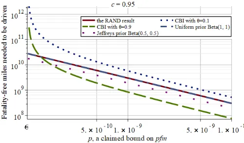
[image:5.612.311.561.49.196.2]The proof of Theorem 1 is in appendix A. Depicted in Fig. 1 are two common situations (given different values of the model parameters): with failure-free and rare failures evidence.
Fig. 1: Conservative two-point priors for two choices of model parameters – with failure free data (left) and rare failures (right).
Solving (3) forn– the miles to be driven to claim thepfmis less thanpwith probabilityc, upon seeingkfailures – provides our main technical result. From a Bayesian perspective, n will depend on the prior knowledge (2). In what follows, we compare the proposednvalues from CBI, the RAND study, a Uniform prior and Jeffreys prior (as suggested by regulatory guidance like [31]). Similar comparisons can be made forpcm; we omit these due to page limitations.
B. Numerical Examples of CBI for pfm Claims
In the RAND study, data from the U.S. department of transportation supported a pfmfor human drivers of1.09e−8
in 2013. For illustration, suppose that a company aims to build AVs two orders of magnitude safer, i.e. = 1.09e−10, as proposed by [39]. Also, assume pl = 10−15: that is, the unknown pfm value cannot be better than10−15.
Q1: How many fatality-free miles need to be driven to claim a pfm bound at some confidence level?
With the prior knowledge (2), we answer Q1 by setting k= 0and solving (3) forn. Fig. 2 shows the CBI results with θ= 0.1 (weak belief) andθ= 0.9 (strong belief) respectively, compared with the RAND results, and Bayesian results with a uniform prior Beta(1,1)and the Jeffreys prior for Binomial models (Beta(0.5,0.5)[31, p.6.37]). Fig. 2 shows that (3) can imply significantly more, or less, miles must be driven than suggested by either the RAND study or the other Bayesian priors – depending on how confident one isbefore seeing test resultsthat the goalhas been reached. For instance, to claim, with 95% confidence, that AVs are as safe as human drivers (so p= 1.09e−8), the RAND analysis requires 275 million fatality-free miles, whilst CBI with θ= 0.9 only requires 69 million fatality-free miles, with 90% prior confidence that the AVs are two orders of magnitude safer than humans (based on, e.g., having the core ML-based systems backed up by non-ML safety channels that are relatively simple and easier to be verified. Such verification can be the case in traditional safety-critical systems [15]).
Alternatively, if one has only a “weak” prior belief in the engineering goal being met (θ= 0.1), then CBI requires 476 million fatality-free miles – significantly more than the other approaches compared.
Fig. 2: Fatality-free miles needed to be driven to demonstrate a
pfmclaim with95% confidence. Note, the curves for Bayes with a uniform prior and the RAND results overlap in the figure (to be exact, there is a constant difference of 1 between them which is simply a consequence of the similarity between their analytical expressions in this scenario).
The reader should not be surprised that our conservative approach does not always prescribe more fatality-free miles be driven than that prescribed by the RAND study – different decision criteria and statistical inference methods can yield different results from the same data [41]. However, it is true that, for any confidencec, CBI will require significantly more miles than the RAND study prescriptions for all claims p “close enough” to the engineering goal.
We note that, for AVs that may have less stringent reliability requirements (e.g. AVs doing regular inspection missions on offshore rigs), both the engineering goal and reliability claims can be much less stringent than the examples in Fig. 2. We present CBI and RAND results for such a scenario in Fig. 3, with an engineering goal = 10−4 and a range [10−4,10−2] for the claimed boundp. Although it shows the same pattern as Fig. 2, the evidence required to demonstrate a reliability claim being met with the given confidence level is much less and within a feasible range. For instance, when the claim of interest is p = 10−3, CBI with a strong prior belief in the engineering goal being met (i.e. θ = 0.9) requires less than
103 failure-free miles, while the RAND method requires 2 to 3 times as many.
Notice that, for all of the scenarios we have presented so far, no amount of testing will support trust in any boundplower than. This is because of constraint (2). It allows a range of possible prior distributions – and thus posterior confidence bounds – but with no added basis for trusting any bound better than(as exemplified in Fig. 2). Hence, a conservative decision maker that has partial prior knowledge (2) cannot accept a claim, on the basis of the fatality-free operation, that the AV reliability exceeds the engineering goal. Of course, if furtherevidence justifies a prior knowledge in some boundp (< ), then CBI can give more informative claims.
Q2: How many miles need to be driven, with fatality events, to claim apfm bound at some confidence level?
[image:5.612.51.299.127.194.2]hy-Fig. 3: Failure-free miles needed to be driven to demonstrate a less stringent reliability claim with95%confidence.
pothesis testing, choosing as an example a confidence bound 20% better than human drivers’ pfmin 2013. Their result (in number of miles required) is shown in boldface in Table. I.
In the Bayesian approach, posterior confidence depends on observations: in order to compare with the RAND study result, we thus postulate an observed number of fatalities consistent with the RAND study analysis. As an example, we consider that, given a pfm equal to the above confidence bound, and driving the number of miles found necessary in the RAND study, the expected number of fatalities would be k = 8.72e−9×4.97e9≈43(where 8.72e−9 is a reliability claim obtained from 4.97e9 fatality free miles in the RAND model). We thus assume 43 fatalities and show in column 1 of Table I the miles required by the Bayesian approaches, including CBI, Uniform and Jeffreys priors. In addition to the purpose of comparison, this case also represents a long term scenario in which, as popularity and public use of AVs grow, the count of fatal accidents progressively reaches high values. We show what evidence would then be needed to reassure the public that reliability claims are still being met.
For a short term scenario, as a second example, the last column of Table I shows the corresponding results, if only one fatality occurs. Again, we compare the results of classical hypothesis testing, CBI and using other Bayesian priors.
All of the examples in Table I “agree”: the miles needed to make these claims are prohibitively high. However, given the CBI prior beliefs, the CBI numbersrequire 10∼20 times more miles than the rest if 43 fatalities are seen. The number at the bottom of column 1 represents the miles needed to demonstrate that, after fatalities consistent with pfm= 8.72e−9, there is only a 5%chance of the truepfm being worse than that. The difference from the RAND results may seem large, but it is in the interest of public safety: CBI avoids implicit, unwittingly optimistic assumptions in the prior distribution.
We recall that with no fatalities, the CBI exampledoesoffer a sound basis for achieving high confidence with substantially fewer test miles than the RAND approach requires (e.g. 69 vs 275 million miles).
Q3: How many more fatality-free miles need to be driven
p=8.72e-9,k=43 p=4.12e-9,k=1
Classical 4.97e9 2.43e8
Uniform priors 6.40e9 1.15e9
[image:6.612.324.546.49.109.2]Jeffreys priors 6.33e9 9.48e8 CBI withθ= 0.9 7.89e10 3.88e9
TABLE I: Miles needed to support apfm claimpwith 95% confi-dence, withkfatalities.
to compensate for one newly observed fatality?
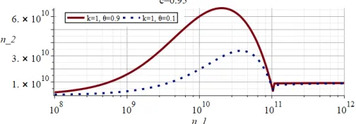
This question relates to a plausible scenario in the case of accidents6: an AV has been driven forn1 fatality-free miles,
justifying a pfm claim, sayp(with a fixed confidence c), via CBI based on this evidence and some given prior knowledge. Then suddenly a fatality event happens. Instead of redesigning the system (as no evidence exists to point to a technical/AI control design fault), the company still believes in its prior knowledge, attributes the fatality to “bad luck” and asks to be allowed more testing to prove its point. If the public/regulators accept this request, it is useful to know how many extra fatality-free miles, say n2, are needed to compensate for the fatality event, so that the company can demonstrate the same reliabilitypwith confidencec.
To answer this, apply the CBI model in two steps (fixing the confidence level c and prior knowledge θ): (i) determine the claim[X6p]that n1will support withk= 0(i.e. fixk, n & solve (3) for p). (ii) determine the miles that support the claim[X6p] upon seeingk= 1 (i.e. fixk, p & solve (3) for n). Then n2=n−n1 more fatality-free miles are needed to compensate for the fatality; we plot some scenarios in Fig. 4.
Fig. 4: Fatality-free miles needed to compensate one newly observed fatality givenn1 fatality-free miles has been driven before.
The solid curve in Fig. 4 shows a uni-modal pattern, decreasing as n1 approaches the value n∗ = 1.06e11 (with a correspondingpvalue,p∗= 1.16e−10, derived from the 1st step), then increasing again with an asymptote of n2 = 1/, asn1goes to infinity. A complete formal analysis derivingp∗ and the asymptote of n2= 1/is in Appendix B.
Intuitively, the more fatality-free miles were driven, the higher one’s confidence in reliability; and thus, the more miles needed to restore that confidence after a fatality occurs. But, ifn1 was such as to allow confidence in a claim close to p1, then after the fatality, a much smallern2is needed to be able to claimp1 again. Asn1 tends to infinity, interestingly, there
[image:6.612.53.297.54.204.2] [image:6.612.312.564.426.514.2]is a ceiling on the required n2,for all values ofc andθ. We note that the shape of the curve (including the asymptote on the right) is invariant with respect to c andθ.
IV. SRGMS FORdpmPREDICTIONS
Whilst the previous sections focused on very rare events like fatalities and crashes, in this section we focus on a metric for a more frequent event, often reported for AV road testing data: disengagements per mile (dpm). Several descriptive statistical studies for dpm exist: e.g., Banerjee and co-authors, using large-scale AV road testing data, show negative correlation betweendpmand cumulative miles driven over three years, but still not reaching AV manufacturers’ targets despite millions of miles driven [8]. As part of road-test planning, any forecast of futuredpmmust account for this trend of apparent improvement.
The idea behind Software Reliability Growth Models (SRGMs) is that each fault contributes to causing failures stochastically during operation. When a failure occurs, the software is updated in an attempt to fix that fault, then use of the software, or testing, resumes until the next failure reveals another fault. During this fault-finding and fixing process, recorded inter-failure times are used to calibrate probabilistic models so as to extrapolate the trend, in probabilistic terms, e.g. predicting the mean, or median, time to the next failure.
Many SRGMs have been developed, based on different assumptions (e.g. how much each fault contributes to the overall failure rate). Comparing them by how plausible their assumptions seem has not proven good guidance, and no single SRGM proved universally accurate [42]. As an alternative, techniques were proposed [43] to assess and compare SRGMs’ prediction accuracyover the history of a specific product. One could thus choose which SRGM to trust, or even “recalibrate” them to improve predictions for that system. Thus, the best practice is to apply multiple SRGMs to the failure data of the system under study, recalibrating them as appropriate, and compare the prediction accuracy, so that we can gradually learn which SRGM seems to be best for the current prediction needs [13].
Statistical properties of AVs, such asdpms, exhibit growth, as training/self-learning is applied after failures occur. We apply various SRGMs to disengagement data, and assess the models’ predictive accuracy. The latter seems even more necessary for AVs, with their ML-based systems, than for conventional software-based systems, as knowledge of AVs’ learning mechanisms is so imperfect (and often not available to third-party assessors) that we cannot choose a priori the most fit SRGM for a given AV.
A. Applying SRGMs to Waymo AVs Data
The California AV Testing Regulations require annual re-ports on disengagements from every manufacturer authorised to test AVs on public roads. We applied SRGMs to the data reported from Waymo covering 51 months of testing, available from Waymo7at the time of writing. We use PETERS, a
state-7www.dmv.ca.gov/portal/dmv/detail/vr/autonomous/testing
of-the-art toolset that implements 8 SRGMs, recalibration, comparison and visualisation techniques. We select the most trustworthy SRGM to predict, after each failure (i.e. disen-gagement), the median miles to next disengagement (MMTD), based on the series of previous inter-failure mile data.
In Fig. 5A,C,E,F, the 528 failures in Waymo’s disengage-ment data are indexed in chronological order on the x-axis8.
Fig. 5A shows the successive MMTD predictions (for a better illustration, we show the results of 5 out of the 8 SRGMs im-plemented in PETERS)9. As is common, the SRGMs disagree:
GO is more optimistic; LV and Li are more pessimistic. To check whether they are objectively optimistic or pessimistic, we use PETERS’u-plotfeature. U-plots show how “unbiased” a set of predictions is: how close the confidence associated to each prediction is to its actual probability of being correct. A point on a u-plot, for a value x on the xaxis, indicates the fraction of predictions for which the predicted probability of the inter-failure miles thatwere observedwas no greater than x. The better calibrated a set of predictions is, the closer the u-plot will be to the diagonal [43].
Fig. 5B shows that most SRGMs proved indeed system-atically too optimistic or pessimistic. The MO predictions seem the best calibrated; however, a good u-plot does not guarantee an SRGM is accurate (or useful) in every way. Next, to reduce bias, we “recalibrate” all models. Recalibration may improve prediction accuracy (in Fig. 5, the # suffix identifies a recalibrated model). Fig. 5C shows that recalibration reduced the disagreement between MMTD predictions. Fig. 5D shows that recalibration drastically reduced bias for most SRGMs (MO# has slightly more pessimistic bias than MO).
To compare these series of predictions by overall accuracy, we use PLR-plots (Fig. 5F). Suppose that two predictors (SRGMs), A and B, give probability density functionsgˆA
j(·) and gˆB
j (·) for the unknown miles to the next failure, given the series of inter-failure miles up to failurej. When a failure does happen, at mj+1, if A is the more accurate predictor, then the ratiogˆjA(mj+1)/gˆjB(mj+1)tends to be larger than 1. The PLR of A relative to B (“A:B” in Fig. 5F) is defined as the running product of such ratios,Qk1 gˆiA−1(mi)/ˆgiB−1(mi)
. If it consistently increases, then A is generally more accurate than B. The PLR-plots in Fig. 5F show that, the four SRGMs that roughly agreed in the MTTD predictions in Fig.5C were, after the 400th failure, generally more accurate (by the same amount: same slope of their PLR-plots) than GO#, an outlier towards optimism in Fig.5C. For this data set, the best estimate of current MMTD (Fig. 5C) is thus about 7-8000 miles. SRGMs arenotsuitable for deciding whether a safety-critical system satisfies requirements (like those for AVs) of very low rates of serious failures. Even if a SRGM’s “accuracy” and
8The raw data are numbers of disengagements, and miles driven, per month; PETERS requires a sequence of inter-failure miles. We preprocessed the raw data by generating random points in a Poisson Process for each month, repeating to check sensitivity of the results to this manipulation.
Fig. 5: MMTD predictions (A, improved in C), u-plots (B and D), PLR plots for SRGMs (and recalibrated SRGMs), applied to Waymo’s 51-month dataset. The SRGMs (plots in A and C) extract predictions about how the trends will continue from the raw data (E); their predictive accuracy can be judged using the other plots.
“calibration” properties have proved good, this cannot give high confidence in the one prediction that matters, the one after thelatest change; that change could have departed from the previous trend – even radically increasing the failure rate – but the SRGM would not “notice” until the next failure. Yet, SRGMs can be a practical management tool for predicting future inter-event intervals, given large amounts of data, as is the case here for dpm. By contrast, the CBI developed in Section III provides a rigorous approach for safety claims about AVs in scenarios with rare failures.
V. RELATEDWORK
CBI was initially developed for assessing the reliability of conventional safety-critical software in [23]. Several exten-sions, e.g. [24]–[26], [38], have been developed, considering different prior knowledge and objective functions. CBI has recently been used for estimating catastrophic failure related parameters in the runtime verification of robots [44].
For conventional software, many SRGMs have been devel-oped [45]. To the best of our knowledge, the only SRGM developed specifically for ML-based software is [46], in which the MO-model was modified to incorporate certain features of
AI software. Differently from [46], our approach is to not trust any specific SRGM, but to assess forecast accuracy, improve forecasts, and identify the best SRGMs for the given data.
Studies in [8], [10]–[12], [36] provide descriptive statistics on AV safety and reliability. Both [9] and [4] conclude that road testing alone is inadequate evidence of AV safety, and argue the need for alternative methods to supplement public road testing. We agree, and our CBI approach provides a concrete way to incorporate such essential prior knowledge into the assessment.
VI. CONCLUSIONS& FUTUREWORK
The use of machine learning (ML) solutions in safety-critical applications is on the rise. This imposes new challenges on safety and reliability assessment. For ML systems, the in-ability to directly verify that a design matches its requirements, by reference to the process of deriving the former from the lat-ter, makes it even harder (compared to conventional software) to estimate the probabilities and consequences of failure [47]. Thus, we believe, increased reliance on operational testing to study failure probabilities and consequences is inevitable.
In the case of AVs, the problem is also one of demonstrat-ing “ultra-high reliability” [13], for which it is well-known that convincing arguments based on operational testingalone are infeasible. While Bayesian inference supports combining operational testing with other forms of evidence, this latter evidence would need to be such as to support very strong prior beliefs. Use of safety subsystems – not relying on the AV’s core ML-based systems – that are verifiable with conventional methods so as to support stronger prior beliefs (than can be had for the ML-based primary system), provides part of the solution. How to support prior beliefs strong enough to give sufficient posterior confidence in the kind of dependability levels now desired for AVs remains an unsolved problem.
Our CBI approach removes the other major difficulty with these problems, that of trusting more detailed prior beliefs than the evidence typically allows one to argue. One can, thus, take advantage of Bayesian combination of evidence (even given few or no failures) while avoiding possible optimistic bias. This does not solve all of the problems of assessing “ultra-high dependability”, but it does allow one to trust Bayesian infer-ence; which will deliver enough confidence when requirements are not so extreme (cf Fig. 3). For non-ultra-high reliability measures that exhibit growth due to “learning” over time, SRGMs, with accuracy validation/recalibration techniques, are useful (at least to derive prior beliefs for inference about reliability of a current version of the AV).
We demonstrate CBI and SRGM methods on one of the most visible examples of an ML-based system with safety-assessment challenges – autonomous vehicles. To recap, the main contributions of this paper are:
which the ML-based system functions are paired with non-ML safety subsystems, where such safety subsystems are sufficient to avoid accidents and can be rigorously verified. Being a Bayesian approach, CBI allows one to “give credit” for this essential evidence. It can thus contribute to overcoming the challenges of supporting extreme reliability claims; while its conservatism avoids the potential for dangerous errors in the direction of optimism, inherent in common shortcuts for applying Bayes in these cases.
b) for extrapolating past disengagement trends, we demon-strate an application of SRGMs to real AV data, with the methods introduced by [28], [48]. Like previous studies on SRGMs, this example emphasises the importance of continu-ously evaluating forecasting accuracy, as various applications have shown that no particular SRGM should be expected to always give the “best” predictions. Even when an SRGM is shown to outperform others, so far, in a sequence of forecasts, such dominance has been known to change with further observations. We also illustrate how systematic shortcomings in past predictive accuracy can be used to, possibly, im-prove the performance of these models by using recalibration techniques. This is important with AV reliability data, given AVs’ evolving/learning nature and the need to drive under (constantly) changing conditions/environments. The methods for evaluation and recalibration are very general; in principle, they may be applied more widely to point processes.
In future work, we plan to explore: (a) methods for rigorous claims based on road testing in diverse environments (e.g. cities, traffic regimes; including the case that road testing is “stratified” with more testing in those conditions that are expected to be more challenging, while the scenario considered here is of testing that statistically matches expected use); (b) assessing any alternative models for reliability growth in ML-based systems, in case they prove to deliver more accurate predictions, and studying their possible role in arguments for high reliability; (c) adapting CBI extensions to support sound decisions about the progressive introduction of AVs [24].
Although we have focused on the “hot” area of AVs, our discussion and the novel CBI theorems are more generally applicable. We see them as especially useful now for ML-based systems with critical applications, although not with ex-treme requirements, since assurance in these systems must rely on combinations of statistical evidence with other verification methods that are, as yet, not well-established.
APPENDIX
A. Statement And Proof of CBI Theorem 1
Problem: Consider the set D of all probability distributions defined over the unit interval, each distribution representing a potential prior distribution of pfm values for an AV. For
0 < pl < 61, we seek a prior distribution that minimises the posterior confidence in a reliability boundp∈[pl,1], given k fatalities have occurred over n miles driven and subject to
constraints on some quantiles of the prior distribution. That is, for θ∈(0,1], we solve
minimise
D P r(X6p|k&n)
subject to P r(X6) =θ, P r(X>pl) = 1 Solution: There is a prior in D that minimises the posterior confidence: the 2-point distribution
P r(X=x) =θ1x=x1+ (1−θ)1x=x3
wherepl6x16 < x3, and the values of x1 andx3 both depend on the model parameters (i.e.pl, , p) as well askand n. Using this prior, the minimum posterior confidence is
xk1(1−x1)n−kθ xk
1(1−x1)n−kθ+x3k(1−x3)n−k(1−θ)
1p> (4)
where1Sis an indicator function – it is equal to 1 when Sis true and 0 otherwise.
Proof. The proof is constructive, starting with any feasible prior distribution and progressing in 3 stages, each stage producing priors that give progressively worse posterior con-fidence than in the previous stage. In more detail, assuming 6p(the argument forp < is analogous):
1) First we show that, for any given feasible prior distribu-tion in D, there is an equivalent feasible 3-point prior distribution. “Equivalent”, in that the 3-point distribution has the same value for the posterior confidence in p as the given feasible prior. Consequently, we restrict the optimisation to the set D∗ of all such 3-point distributions;
2) For each prior in D∗, there exists a 2-point prior distribution with a smaller posterior confidence in p. Consequently, we restrict the optimisation to the setD∗∗ of all such 2-point priors;
3) A monotonicity argument determines a 2-point prior in
D∗∗ with the smallest posterior confidence in p. Stage 1: Assuming6p, note that for any prior distribution F ∈ D, we may write
P r(X 6p|k&n) = T
T+R1
p+xk(1−x)n−kdF(x)
(5)
whereT=R plx
k(1−x)n−kdF(x) +Rp
+xk(1−x)n−kdF(x).
Themean-value-theorem for integralsensures that three points exist, x1 ∈ [pl, ], x2 ∈ (, p] and x3 ∈ (p,1], such that (5) becomes (denote Rp
+dF(x) =β):
xk
1(1−x1)n−kθ+xk2(1−x2)n−kβ xk
1(1−x1)n−kθ+xk2(1−x2)n−kβ+xk3(1−x3)n−k(1−θ−β) (6)
Stage 2: Next, for each prior in D∗, there is a 2-point prior distribution that is guaranteed to give a smaller posterior confidence in p. To see this for any given prior in D∗ with posterior (6), treat all of the other variables as fixed (i.e. the “x”s andθ) and consider which of the allowed values forβ, given these fixed values of the other variables, guarantees a distribution that reduces the posterior confidence. The continu-ous differentiability of rational functions – of which (6) is one – allows the partial derivative of (6) w.r.t. β to show us the way to do this. The partial derivative of (6) with respect to β is always positive, irrespective of the fixed values thexis take in their respective ranges. So, to minimise (6), we set β= 0. This gives the attainable lower bound (7), attained by the 2-point prior distribution with probability masses θ at x=x1, and 1−θ atx=x3. Therefore, we restrict the optimisation toD∗∗ – the set of all such priors.
P r(X6p|k&n)> x
k
1(1−x1) n−kθ xk
1(1−x1)n−kθ+x3k(1−x3)n−k(1−θ)
= 1
1 +xk3(1−x3)n−k
xk
1(1−x1)n−k
1−θ
θ
(7)
Stage 3: To minimise (7) further (and, thereby, obtain optimal priors in D∗∗), we maximise xk
3(1 −x3)n−k and minimise xk
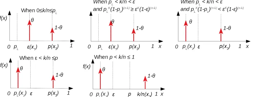
1(1−x1)n−k over the allowed ranges for x1, x3. The problem is now reduced to a simple monotonicity analysis given different values of the other model parameters, as follows. Since xk(1−x)n−k is bell-shaped over [0,1] with a maximum at x=k/n, the following defines 2-point priors that solve the optimisation problem (depicted in Fig 6):
• When06k/n6pl: to minimise xk
1(1−x1)n−k, subject tox1 ∈[pl, ], we set x1=;
to maximise xk
3(1−x3)n−k, subject to x3∈(p,1], we set x3=p.
• Whenpl< k/n6, andpkl(1−pl)n−k>k(1−)n−k: to minimise xk1(1−x1)n−k, subject tox1 ∈[pl, ], we set x1=;
to maximise xk3(1−x3)n−k, subject to x3∈(p,1], we set x3=p.
• Whenpl< k/n6, andpkl(1−pl)n−k< k(1−)n−k: to minimise xk
1(1−x1)n−k, subject tox1 ∈[pl, ], we set x1=pl;
to maximise xk
3(1−x3)n−k, subject to x3∈(p,1], we set x3=p.
• When < k/n6p: to minimise xk
1(1−x1)n−k, subject tox1 ∈[pl, ], we set x1=pl;
to maximise xk
3(1−x3)n−k, subject to x3∈(p,1], we set x3=p.
• Whenp < k/n61:
to minimise xk1(1−x1)n−k, subject tox1 ∈[pl, ], we set x1=pl;
to maximise xk3(1−x3)n−k, subject to x3∈(p,1], we set x3=k/n.
Each prior above has the form (4) for P r(X 6p|k&n).
All of the foregoing proves Theorem 1 for6p. Begin the optimisation again, but now assumingp < . For any feasible priorF∈ D, the objective functionP r(X 6p|k&n)can be written as
L L+R
p+xk(1−x)n−kdF(x) +
R1
+xk(1−x)n−kdF(x)
(8)
whereL=Rp plx
k(1−x)n−kdF(x). As before, the
mean-value-theoremensures the existence of three pointsx1, x2, x3 in the ranges:x1∈[pl, p], x2∈(p, ], x3∈(,1]such that (8) becomes (denote Rp
pldF(x) =γ, where 06γ6θ):
L0 L0+xk
2(1−x2)n−k(θ−γ) +xk3(1−x3)n−k(1−θ) (9)
whereL0=xk1(1−x1)n−kγ.
The derivative of (9) with respect to γ is always positive, irrespective of the fixed values thexis can take in their allowed ranges. So, to minimise (9), we simply setγ= 0. Thus, (9) has an attainable bound of 0 when p < , and the corresponding prior distribution that attains this is still a 2-point one with probability masses at x=x2 andx=x3, regardless of what fixed valuesx2 andx3 take in their allowed ranges.
B. Formal Analysis for Q3 in Sec. III-B
We seek to understand what happens when n1 fatality-free driven miles support a pfm claim p with confidence c. And, upon seeing a fatality after n1 miles, understanding how many more fatality-free milesn2are needed to maintain support for the claim. So, what follows is an analysis of the asymptotic “largen” behaviour implied by the worst-case posterior confidence (3) in Theorem 1. Assume c and θ are given in the practical case whenc>θ.
Let n∗ denote the number of miles that satisfies (1 −
)n∗−1 = p
l(1−pl)n
∗−1
. So, from appendix A above, for n < n∗ we have x1 =pl, and for n>n∗ we have x1 =. Note that n∗ is independent of c and θ, so this number of miles will be the same no matter what levels of confidence one is either interested in, or has prior to road testing.
Now, using (3), we may write the number of miles driven as a function of the remaining problem parameters. That is, for < p61,
n(c, p, θ, x1, k) :=k+
klog(x1/p) + log( θ(1−c) c(1−θ))
log(11−−xp
1)
(10)
where we have assumed that the values ofnensurek/n6p holds. In particular, fork= 1, letp∗ uniquely satisfy
n∗= 1 +
log(x1/p∗) + log(θc(1(1−−θc))) log(11−−px∗
1)
(11)
Fig. 6: The 5 possible cases of two-point prior distributions that minimise (5). Notice the important role of wherek/nlies.
If, for otherwise fixed parameter values, we denote n˜ the number of miles according to (10) when k = 1, and n1 the number of miles when k= 0, then the number of additional miles n2 needed upon seeing a fatality immediately aftern1 miles isn2:= ˜n−n1.
Suppose then, that p > p∗ and letptend top∗ from above. The following limits follow from the continuity ofn in (10): 1) If a fatality is observed (so k= 1) then, as ptends to p∗ from above, we have x1 = pl, and the number of miles that are needed to be driven to support a claim in p – with confidence c using prior confidence θ in the engineering goalbeing met – is
lim
p↓p∗n˜= limp↓p∗n(c, p, θ, pl,1)
=n(c,lim
p↓p∗p, θ, pl,1) =n(c, p
∗, θ, p
l,1) =n∗ 2) If no fatalities are observed (sok= 0)then, asptends
top∗ from above, the number of fatality-free miles that are needed to be driven to support a claim inp– with confidencecusing prior confidenceθin the engineering goalbeing met – is
lim
p↓p∗n1= limp↓p∗n(c, p, θ, ,0) =n(c,plim↓p∗p, θ, ,0)
=n(c, p∗, θ, ,0) =
log(θc(1(1−−θc))) log(11−−p∗)
Recall, from appendix A, that x1 = must hold here for allpwhen k= 0.
3) so, using these last two results, the number of extra miles needed is
lim
p↓p∗n2=n
∗−log(
θ(1−c) c(1−θ))
log(11−−p∗) (12)
Alternatively, suppose p < p∗ and let p tend to from above. The following limits also follow from (10):
1) If a fatality is observed (so k = 1), then as p tends to from above, we have x1 =, and the number of miles that are needed to be driven to support a claim in
p – with confidence c using prior confidence θ in the engineering goalbeing met – is
lim
p↓n˜= limp↓n(c, p, θ, ,1) =n(c,limp↓p, θ, ,1) =∞ 2) If no fatalities are observed (so k= 0)then, asptends
to from above, the number of fatality-free miles that are needed to be driven to support a claim in p– with confidencecusing prior confidenceθin the engineering goal being met – is
lim
p↓n1= limp↓n(c, p, θ, ,0) =n(c,limp↓p, θ, ,0) =∞ 3) the last two results show that both n˜ and n1 grow
without bound, however the number of extra miles needed is bounded above, since (byL’Hospital’s rule)
lim
p↓n2= limp↓(˜n−n1)
= lim
p↓(n(c, p, θ, ,1)−n(c, p, θ, ,0))
= 1 + lim
p↓
log(/p) log(11−−p)
!
= 1 + lim
p↓
(1/p)
1/(1−p) = 1 + 1−
= 1/ (13) Note that, liken∗, this limit is independent of candθ.
REFERENCES
[1] J. M. Anderson, K. Nidhi, K. D. Stanley, P. Sorensen, C. Samaras, and O. A. Oluwatola, “Autonomous vehicle technology: A guide for policymakers,” Rand Corporation, Tech. Rep. RR-443-2-RC, 2016. [2] B. Paden, M. ˇC´ap, S. Z. Yong, D. Yershov, and E. Frazzoli, “A survey of
motion planning and control techniques for self-driving urban vehicles,”
IEEE Tran. on Intelligent Vehicles, vol. 1, no. 1, pp. 33–55, 2016. [3] D. J. Fagnant and K. Kockelman, “Preparing a nation for autonomous
vehicles: Opportunities, barriers and policy recommendations,”Transp. Research Part A: Policy and Practice, vol. 77, pp. 167–181, 2015. [4] P. Koopman and M. Wagner, “Autonomous vehicle safety: An
interdis-ciplinary challenge,”IEEE Intelligent Transportation Systems Magazine, vol. 9, no. 1, pp. 90–96, 2017.
[7] C. Urmson, “Hands off: The future of self-driving cars,” Committee on Commerce, Science and Transportation, Washington, D.C., USA, Testimony, 2016.
[8] S. S. Banerjee, S. Jha, J. Cyriac, Z. T. Kalbarczyk, and R. K. Iyer, “Hands off the wheel in autonomous vehicles?: A systems perspective on over a million miles of field data,” in48th IEEE/IFIP Int. Conf. on Dependable Systems and Networks, 2018, pp. 586–597.
[9] N. Kalra and S. Paddock, “Driving to safety: How many miles of driving would it take to demonstrate autonomous vehicle reliability?”Transp. Research Part A: Policy and Practice, vol. 94, pp. 182–193, 2016. [10] F. Favar`o, S. Eurich, and N. Nader, “Autonomous vehicles’
disengage-ments: Trends, triggers, and regulatory limitations,”Accident Analysis & Prevention, vol. 110, pp. 136 – 148, 2018.
[11] V. V. Dixit, S. Chand, and D. J. Nair, “Autonomous vehicles: Disen-gagements, accidents and reaction times,”PLOS ONE, vol. 11, no. 12, pp. 1–14, 2016.
[12] C. Lv, D. Cao, Y. Zhao, D. J. Auger, M. Sullman, H. Wang, L. M. Dutka, L. Skrypchuk, and A. Mouzakitis, “Analysis of autopilot disengagements occurring during autonomous vehicle testing,” IEEE/CAA Journal of Automatica Sinica, vol. 5, no. 1, pp. 58–68, Jan. 2018.
[13] B. Littlewood and L. Strigini, “Validation of ultra-high dependability for software-based systems,”Comm. of the ACM, vol. 36, pp. 69–80, 1993. [14] R. W. Butler and G. B. Finelli, “The infeasibility of quantifying the reliability of life-critical real-time software,” IEEE Transactions on Software Engineering, vol. 19, no. 1, pp. 3–12, Jan. 1993.
[15] B. Littlewood and J. Rushby, “Reasoning about the reliability of diverse two-channel systems in which one channel is ‘possibly perfect’,”IEEE Tran. on Software Engineering, vol. 38, no. 5, pp. 1178–1194, 2012. [16] Waymo, “Waymo safety report: On the road to fully self-driving,”
Tech. Rep., 2018. [Online]. Available: https://storage.googleapis.com/ sdc-prod/v1/safety-report/SafetyReport2018.pdf
[17] A. Shashua and S. Shalev-Shwartz, “A plan to develop safe autonomous vehicles. And prove it,” Intel Newsroom, p. 8, 2017. [Online]. Available: https://newsroom.intel.com/newsroom/wp-content/ uploads/sites/11/2017/10/autonomous-vehicle-safety-strategy.pdf [18] Y. Tian, K. Pei, S. Jana, and B. Ray, “DeepTest: Automated testing of
deep-neural-network-driven autonomous cars,” inthe 40th Int. Conf. on Software Engineering, New York, NY, USA, 2018, pp. 303–314. [19] M. Kamali, L. A. Dennis, O. McAree, M. Fisher, and S. M. Veres,
“Formal verification of autonomous vehicle platooning,” Science of Computer Programming, vol. 148, pp. 88 – 106, 2017.
[20] M. Fisher, E. Collins, L. Dennis, M. Luckcuck, M. Webster, M. Jump, V. Page, C. Patchett, F. Dinmohammadi, D. Flynn, V. Robu, and X. Zhao, “Verifiable self-certifying autonomous systems,” inIEEE Int. Symp. on Software Reliability Engineering Workshops, 2018, pp. 341–348. [21] P. Koopman and B. Osyk, “Safety argument considerations for public
road testing of autonomous vehicles,” inWCX SAE World Congress Experience. SAE International, Apr. 2019.
[22] P. Popov and L. Strigini, “Assessing asymmetric fault-tolerant software,” inthe 21st Int. Symp. on Software Reliability Engineering. San Jose, CA, USA: IEEE Computer Society Press, 2010, pp. 41–50.
[23] P. Bishop, R. Bloomfield, B. Littlewood, A. Povyakalo, and D. Wright, “Toward a formalism for conservative claims about the dependability of software-based systems,”IEEE Transactions on Software Engineering, vol. 37, no. 5, pp. 708–717, 2011.
[24] L. Strigini and A. Povyakalo, “Software fault-freeness and reliability predictions,” inComputer Safety, Reliability, and Security, ser. LNCS, vol. 8153. Springer Berlin Heidelberg, 2013, pp. 106–117.
[25] X. Zhao, B. Littlewood, A. Povyakalo, L. Strigini, and D. Wright, “Modeling the probability of failure on demand (pfd) of a 1-out-of-2 system in which one channel is “quasi-perfect”,”Reliability Engineering & System Safety, vol. 158, pp. 230–245, 2017.
[26] X. Zhao, B. Littlewood, A. Povyakalo, and D. Wright, “Conservative claims about the probability of perfection of software-based systems,” in
26th Int. Symp. on Software Reliability Eng. IEEE, 2015, pp. 130–140. [27] D. R. Miller, “Exponential order statistic models of software reliability growth,”IEEE Tran. on Software Eng., vol. 12, no. 01, pp. 12–24, 1986. [28] S. Brocklehurst and B. Littlewood, “Techniques for prediction analysis and recalibration,” inHandbook of Software Reliability Eng., M. Lyu, Ed. McGraw-Hill & IEEE Computer Society Press, 1996, pp. 119–166. [29] IEC, IEC61508, Functional Safety of Electrical/
Elec-tronic/Programmable Electronic Safety Related Systems, 2010.
[30] CENELEC,EN50129, Railway Applications-Communication, Signalling and processing Systems-Safety Related Electronic Systems for Sig-nalling, 2003.
[31] C. Atwood, J. LaChance, H. Martz, D. Anderson, M. Englehardt, D. Whitehead, and T. Wheeler, “Handbook of parameter estimation for probabilistic risk assessment,” U.S. Nuclear Regulatory Commission, Washington, DC, Report NUREG/CR-6823, 2003.
[32] L. Strigini and B. Littlewood, “Guidelines for statistical testing,” City University London, Project Report PASCON/WO6-CCN2/TN12, 1997. [33] G. Walter, L. J. M. Aslett, and F. P. A. Coolen, “Bayesian nonpara-metric system reliability using sets of priors,”International Journal of Approximate Reasoning, vol. 80, pp. 67–88, 2017.
[34] P. Bishop and A. Povyakalo, “Deriving a frequentist conservative confidence bound for probability of failure per demand for systems with different operational and test profiles,”Reliability Engineering & System Safety, vol. 158, pp. 246–253, 2017.
[35] L. V. Utkin and F. P. A. Coolen, “Imprecise probabilistic inference for software run reliability growth models.”Journal of Uncertain Systems., vol. 12, no. 4, pp. 292–308, 2018.
[36] F. M. Favar`o, N. Nader, S. O. Eurich, M. Tripp, and N. Varadaraju, “Ex-amining accident reports involving autonomous vehicles in California,”
PLOS ONE, vol. 12, no. 9, pp. 1–20, 2017.
[37] E. Cinlar,Introduction to Stochastic Processes, ser. Dover Books on Mathematics Series. Dover Publications, Incorporated, 2013. [38] X. Zhao, B. Littlewood, A. Povyakalo, L. Strigini, and D. Wright,
“Conservative claims for the probability of perfection of a software-based system using operational experience of previous similar systems,”
Reliability Engineering & System Safety, vol. 175, pp. 265 – 282, 2018. [39] P. Liu, R. Yang, and Z. Xu, “How safe is safe enough for self-driving
vehicles?”Risk Analysis, vol. 39, no. 2, pp. 315–325, 2019.
[40] E. Awad, S. Dsouza, R. Kim, J. Schulz, J. Henrich, A. Shariff, J.-F. Bonnefon, and I. Rahwan, “The Moral Machine experiment,” Nature, vol. 563, no. 7729, pp. 59–64, 2018.
[41] J. O. Berger, “Could Fisher, Jeffreys and Neyman have agreed on testing?”Statistical Science, vol. 18, no. 1, pp. 1–32, 2003.
[42] A. A. Abdel-Ghaly, P. Y. Chan, and B. Littlewood, “Evaluation of com-peting software reliability predictions,”IEEE Transactions on Software Engineering, vol. SE-12, no. 9, pp. 950–967, 1986.
[43] S. Brocklehurst and B. Littlewood, “New ways to get accurate reliability measures,”IEEE Software, vol. 9, pp. 34–42, 1992.
[44] X. Zhao, V. Robu, D. Flynn, F. Dinmohammadi, M. Fisher, and M. Web-ster, “Probabilistic model checking of robots deployed in extreme environments,” in Proc. of the 33rd AAAI Conference on Artificial Intelligence, vol. 33, Honolulu, Hawaii, USA, 2019, pp. 8076–8084. [45] M. Xie,Software reliability modelling. World Scientific, 1991, vol. 1. [46] F. B. Bastani, I.-R. Chen, and T.-W. Tsao, “A software reliability model for artificial intelligence programs,”Int. Journal of Software Engineering and Knowledge Engineering, vol. 3, no. 01, pp. 99–114, 1993. [47] Johnson, C. W., “The increasing risks of risk assessment: On the rise of
artificial intelligence and non-determinism in safety-critical systems,” in
the 26th Safety-Critical Systems Symposium. York, UK.: Safety-Critical Systems Club, 2018, p. 15.