City, University of London Institutional Repository
Citation
:
Guimera Busquets, J., Alonso, E. and Evans, A. (2018). Air itinerary shares estimation using multinomial logit models. Transportation Planning and Technology, 41(1), pp. 3-16. doi: 10.1080/03081060.2018.1402742This is the accepted version of the paper.
This version of the publication may differ from the final published
version.
Permanent repository link:
http://openaccess.city.ac.uk/18606/Link to published version
:
http://dx.doi.org/10.1080/03081060.2018.1402742Copyright and reuse:
City Research Online aims to make research
outputs of City, University of London available to a wider audience.
Copyright and Moral Rights remain with the author(s) and/or copyright
holders. URLs from City Research Online may be freely distributed and
linked to.
City Research Online: http://openaccess.city.ac.uk/ [email protected]
1
Air Itinerary Shares estimation using Multinomial Logit Models
1
Ms. Judit Guimera Busquets
12
Department of Mechanical Engineering & Aeronautics, City, University of London,
3
EC1V 0HB London, United Kingdom
4
Dr. Eduardo Alonso
5Department of Computer Science, City, University of London, EC1V 0HB London,
6
United Kingdom
7
Dr. Antony D. Evans
8Crown Consulting, Inc., Moffett field, CA 94035, USA
9
1 Corresponding author: Judit Guimera Busquets
2
Air Itinerary Shares estimation using Multinomial Logit Models
10
The main goal of this study is the development of an aggregate air itinerary
11
market share model. In order to achieve this, multinomial logit models are
12
applied to distribute the city-pair passenger demand across the available
13
itineraries. The models are developed at an aggregate level using open-source
14
booking data for a large group of city-pairs within the US Air Transport System.
15
Although there is a growing trend in the use of discrete choice models in the
16
aviation industry, existing air-itinerary share models are mostly focused on
17
supporting carrier decision-making. Consequently, those studies define itineraries
18
at a more disaggregate level, using variables describing airlines and time
19
preferences. In this study, we define itineraries at a more aggregate level, i.e., as a
20
combination of flight segments between an origin and destination, without further
21
insight into service preferences. Although results show some potential for this
22
approach, there are challenges associated with prediction performance and
23
computational intensity.
24
Keywords: word; air itinerary shares; discrete choice models; multinomial logit;
25
aggregation level;
26
1. Introduction
27
Good forecasts of future demand for air traffic as well as good forecasts of how airlines 28
are likely to serve this demand are essential to enable supply to adapt to growth in 29
demand. While the majority of existing research focuses on improving air travel 30
demand models, there is a growing interest in developing better itinerary share models 31
than those that already exist. Itinerary share models can be crucial to support airline 32
network planning and scheduling since important decisions on resources allocation and 33
pricing are made based on itinerary demand. These decisions are essential as airlines 34
plan their operations, purchase equipment and make strategic decisions. Airport 35
authorities also benefit from good forecasts, given the long timescales associated with 36
3 models is therefore a powerful tool for airline and airport authority planning and 38
decision making, translating into more efficient operations, improved revenue 39
management and increase profitability. Consequently, for the past 15 years, efforts have 40
focused on developing this type of model, shifting away from the Quality of Service 41
indices (QSI) used during the period when the industry was regulated, and/or more 42
simplistic approaches – such as time-series and simplistic probability models based on 43
historical trends – (Garrow, 2010). In contrast, discrete choice models model demand by 44
capturing how individuals make decisions and trade-offs among airports, airlines, price, 45
level of service and other factors that define the air passenger journey. 46
Most of the current research centres on developing innovative approaches using 47
such discrete choice modelling. These approaches, which aim to model competition and 48
customer behaviour to determine air-travel itinerary shares (also known as demand 49
assignment models), are expected to more accurately predict air travel demand. While 50
most of the discrete choice models applied in urban transport are built using 51
disaggregate data and include information about the individual making the decision – 52
i.e. the passenger –; in air transport, data disaggregation as well as data accessibility are 53
limiting factors. The need to quickly adapt to changes in demand makes flexibility 54
crucial for carriers and other stakeholders in the industry. For this reason, most of the 55
models built to support decision-making rely on booking data, which is generally 56
proprietary. Furthermore, airlines do not typically record much of the passenger data 57
that is relevant to passenger decision making, such as age, gender and income. This data 58
is not typically available, except for a small subset of passengers through surveys, 59
which are time consuming and costly to complete. 60
Most of the early studies on demand assignment for air travel focus on studying 61
4 passenger choice in terms of one single criteria, such as airport-choice or airline choice. 63
These early models were mostly applied to analyse air travellers’ choice within multi-64
airport cities or regions – i.e., airport choice models (Hansen, 1995; Windle & Dreesner, 65
1995) – or across airlines – airline choice models (Proussaloglou & Koppelman, 1995) 66
–. Although the former is the most widely studied topic in discrete choice modelling 67
within air transport, and has given a deeper understanding to the relationship between 68
airport attributes and airport market share, a more aggregated assignment of air travel 69
volume is also needed. Only a few studies present approaches for itinerary market share 70
estimation across multiple dimensions (i.e., modelling a passenger's simultaneous 71
choice in terms of multiple criteria, e.g., airline, flight time, fare-class etc.) using 72
discrete choice modelling. Of those, early models used a multinomial logit (MNL) 73
approach (Adler, 2001; Coldren et al., 2003; Grosche and Rothlauf, 2007; Atasoy and 74
Bierlaire, 2012), while more recent models also apply nested logit (NL) models 75
(Coldren and Koppelman, 2005; Hsiao and Hansen, 2011), mixed multinomial logit 76
(MMNL) models (Warburg et al., 2006) and other alternatives approaches (Gramming 77
et al. 2005; Carrier, 2008). The mentioned aggregate passenger-allocation studies can 78
be classified according to the type of data they are based on: revealed preference data 79
(RP) or booking data; stated preferences (SP) data or survey data; or a combination of 80
both. Studies using RP data do not usually provide full insight into passenger choice 81
behaviour since models are estimated based on real booking data, and no information 82
regarding other alternatives at the moment of booking is generally available. This 83
limitation often leads to RP models performing poorly due to the high demand 84
inelasticity of the booking data used to estimate the model (Garrow, 2010). In contrast, 85
SP data collected from surveys allows for modelling of new non-existing alternatives, as 86
5 trips. However, studies using SP data may be subject to bias due to the nature of the 88
experiment in which the individuals are asked to make hypothetical choices by making 89
trade-offs among the attributes of the choice set (e.g., level of service, air fare etc.). 90
Although such surveys provide a customer response to a wider range of choices, 91
providing a better estimate of how individuals make tradeoffs, they are tailored to the 92
needs of the survey writer, which limits the natural range of choice sets to only those 93
that the survery writer is aware of (Garrow , 2010; Louviere et al., 1999). Studies based 94
on SP data are also often limited to a small range of markets, limiting their application 95
to a small network set. 96
Although the models applied in the studies described above are generally 97
effective for the purposes to which they are applied, they do not allow for an estimation 98
of how passenger market demand is distributed across the available itineraries at the 99
most aggregate level, only considering average market air fare and travel time, level of 100
service and basic airport attributes as inputs. 101
This paper presents the full air itinerary share model introduced by Busquets et
102
al. (2016), refined to better capture passenger choice effects, model validation, and 103
estimated at the most aggregate level possible, linking annual city-pair demand to the 104
different itineraries available within the entire US Air Transport System (ATS). 105
The remainder of the paper is structured as follows: The paper’s objectives are 106
presented in Section 2. The modelling approach is detailed in Section 3, with 107
information regarding the input variables used to estimate the model. The model is 108
estimated on one dataset, and validated on another. Section 4 provides information 109
about these two datasets. Modelling results are presented in Section 5, followed by the 110
6
2. Objectives
112
The primary objective of this research is to develop an air itinerary choice model to 113
directly estimate the distribution of passenger demand across available routes for a 114
given O-D pair, using only aggregate data describing average air fare and travel time, 115
level of service and basic airport characteristics. Ultimately, this model will be 116
combined with models for forecasting air travel demand and air traffic, all within the 117
same 3-stage framework (described in Busquets et al., (2015)). This framework consists 118
of the following stages: 119
(1) Forecast city-pair passenger demand; 120
(2) Distribute this demand across available itineraries; and 121
(3) Forecast air traffic as a function of route demand. 122
This modelling approach is inspired by previous research that focused on 123
improving the Federal Aviation Administration's (FAA) forecasting methodology and 124
for which further potential improvements have been identified. The 3-stage framework 125
is expected to allow for identification of the key drivers of evolution in the US ATS as 126
well as to predict future air traffic growth within the US ATS. In order to achieve these 127
objectives, the approach includes three elements beyond that of the existing research: 128
• The use of data mining techniques to model the US ATS evolution in order to 129
predict air traffic with improved accuracy and precision levels while maintaining 130
the simplicity if existing econometrics, gravity and time-series models. 131
• The consideration of a larger set of explanatory variables than is typically 132
considered in existing air traffic forecasting approaches. 133
• Explicitly modelling the distribution of city-pair passenger demand between 134
7 This paper addresses the last of these three elements, which develops the 136
framework’s stage 2 – to distribute passenger demand across available itineraries. The 137
approach described in this paper is therefore expected to: 138
• Highlight the most important factors underlying the air traveller’s choice 139
behaviour within the domestic US ATS; 140
• Perform air itinerary share model refinement and verification for the entire US 141
ATS following previously work (Busquets et al., 2016); and 142
• Explicitly model the distribution of city-pair passenger demand between 143
itineraries within the US ATS. 144
The model presented in this paper is expected to generate better predictions of airport-145
pair air traffic flows once integrated with the air traffic demand model presented by 146
Busquets et al., (2015). 147
3. Approach
148
Data
149
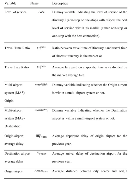
Based on the literature review, there are a large number of factors that describe an 150
itinerary. An itinerary, as defined in this paper, is a flight segment or combination of 151
flight segments connecting a given city-pair. In this study, itineraries are either non-152
stop, or one-stop (i.e., a combination of two flight segments involving an aircraft change 153
during the connection). Considering constraints in data availability and the different 154
attributes that are considered to contain the most relevant information for an itinerary, 155
the input variables for the itinerary market share model are chosen as described in Table 156
1. 157
8 The output variable for the model developed in this paper is the market share (Si)
159
of a given itinerary i. This is defined as the ratio of the demand of the itinerary i (di), to
160
the total demand for the market served by itinerary i (Dm), as shown in Eq. (1). The total
161
demand for market m is given by the sum of passengers travelling on all itineraries that 162
serve that market. 163
𝑆! =!!!
! (1)
164
Detailed Forecasting Methodology
165
Following the work presented by Busquets et al. (2015), which introduced the 3-stage 166
model described in §2 to forecasting future air traffic levels, this paper focuses on fully 167
developing its stage 2 – to distribute passenger demand across available itineraries. The 168
objective of this phase is therefore to transform Origin-Destination (O-D) demand by 169
city-pair into passenger demand by airport-pair using an air itinerary choice model. 170
Stage 2 of the 3-stage model described by Busquets et al. (2015) consists of 2 171
steps: identification of available itineraries estimated using logistic regression 172
(described in detail in Busquets et al. (2015)), followed by the distribution of the O-D 173
demand by city-pair obtained from the O-D demand model (stage 1 in the 3-stage model 174
described by Busquets et al. (2015)) across the available itineraries using a discrete 175
choice model. The first step is motivated by the scope of this research to improve the 176
current FAA's forecasting methodology while maintaining the simplicity of current 177
models and is inspired by a previous research (Kotegawa, 2012). The second step is the 178
focus of this paper. This air itinerary model allows the flight segment passenger demand 179
by airport-pair to be estimated, based on the passenger itinerary demand from all O-D 180
city-pairs. It is not feasible to develop a model for each possible O-D market, so in 181
9 Coldren, et al. (2003): four Continental time zones (Central, East, Mountain and West) 183
and a region for Alaska and Hawaii. This specific O-D market grouping is an attempt to 184
capture similarities among all city-pairs. The number and nature of these regional 185
clusters will be modified using clustering techniques in future work. Given these 186
regions, 18 region-pairs have been defined considering all 16 possible combinations of 187
the Continental time zones – e.g., Central (C-C), East (C-E), Central-188
Mountain (C-M), Central-West (C-W), etc., West-Mountain (W-M), West-West (W-W) 189
–; as well as a pair for Alaska and Hawaii to the Continental US and an region-190
pair for the Continental US to Alaska and Hawaii. For each region-pair, henceforth 191
referred to as an 'entity', an air itinerary share model is developed. 192
This attempts to model the aggregate share of all or groups of decision makers - 193
i.e., air travellers - choosing each alternative as a function of the trip characteristics. In 194
constrast to existing research, the itinerary share estimation is done at the most 195
aggregate level, without considering variables specific to the traveller, such as 196
passenger preferences and perceptions, or variables specific to the service provider, 197
such as airline operating the given route, departure time or aircraft type, among others. 198
Instead, only attributes related to average air fare and travel time, level of service and 199
basic airport characteristics are considered. The focus of the model is to estimate the 200
distribution of annual passenger market demand among itineraries, which will be used 201
as one of the input variables in the third stage of the air traffic estimation model 202
described in §2, per annum. 203
In order to develop the air itinerary share model, RP data is used, avoiding the 204
risk of response bias and allowing for the consideration of a much larger network of 205
city-pairs within the US ATS. The RP data used is 10% ticket survey of booking data 206
10 city-pairs considered, M, are all within the domestic US ATS and are defined by origin 208
and destination. The universal choice set, C, is formed for all possible itineraries within 209
the entire ATS connecting these city pairs. The choice problem is defined for each city-210
pair, m ϵ M, with the choice set being all the possible itineraries connecting that given 211
city-pair, represented by Im. Each itinerary i is characterised by a set of attributes such
212
as level of service, price, time and basic airport characteristics. As a simplification, only 213
two possible levels of service are considered, non-stop and stop flights. For the one-214
stop flights, the connections available are through one of a set of 24 US hub airports 215
defined for this study. 216
The annual share of passenger demand assigned to each itinerary between a 217
given city-pair is modelled as an aggregate multinomial logit (MNL) function and is 218
given by Eq. (2) where Si is the passenger share assigned to itinerary i, Vi is the utility
219
function or value of itinerary i and the summation is over all itineraries for a given city-220
pair. The utility function (Vi) is a linear function of the explanatory variables and
221
assumes that each vector of attributes characterizing an alternative can be reduced to a 222
scalar value, which expresses the attractiveness of each alternative. Consequently, it is 223
expected that the individual or group of individuals will choose the alternative with the 224
highest value, maximizing their utility. Equation (3) shows the general expression for 225
Vi, where Xi is the vector of attributes defining alternative i; and β' represents the
226
coefficients to be estimated capturing the influence of the corresponding attribute on the 227
alternative i (Atasoy & Bierlaire, 2012). 228
𝑆! = !"#!"#(!(!!)
!)
! (2)
229
𝑉! =𝛽!∙𝑋
! =𝛽!∙𝑋!!+𝛽!∙𝑋!!+...+𝛽!∙𝑋!" (3)
11 Attributes included in the Xi vector are described in Table 1 (§3). Some interactions
231
between the attributes are accounted for by the model. After evaluating several model 232
specifications, the interactions that define the utilities considered in this paper were 233
identified as follows: 234
• Accessibility: The interaction between airport accessibility information and 235
multi-airport city information is accounted for (i.e., the masORIG and masDEST
236
variables). Four possible interactions are possible, two regarding the origin 237
airport and two regarding the destination airport. However, because coefficients 238
need to be normalised, the coefficients regarding accessibility for origin and 239
destination airports within cities that are not multi-airport systems are set to 0. 240
• From/to hub variables: The interaction between the hub variables (i.e., whether 241
the itinerary is from and to a hub, only the origin or destination airport is a hub, 242
or none of the itinerary airports are hubs) and markets that contain at least one 243
non-stop itinerary is considered. From/to hub variables are normalised by setting 244
the variable from and to a hub (i.e., the hub2hub variable) to 0. 245
During the estimation of the model, for each city-pair considered, the utility and 246
likelihood function are computed, with the latter being used to calculate the final 247
estimated log likelihood. 248
Although all 18 air-itinerary share models have been developed, in this paper 249
estimated results are only presented for six entities (the entities C-M, M-C, C-W, W-C, 250
M-W and W-M). Due to issues with computational intensity during the estimation 251
process for some entities, reduced estimation datasets were generated by sampling a 252
subset of the total number of city-pairs within the given entity. The size of the reduced 253
12 obtained when considering different estimation dataset sizes. Due to the aggregate 255
nature of the data used in this study and the fact that this data represents only a 10% 256
sample of real booking data, limiting assumptions are implicitly included when 257
estimating the model. For example, some itineraries have a very small probability of 258
occurring, heavily influencing the results obtained for the model estimated as well as its 259
performance. Moreover, due to the large number of city-pairs considered in the 260
estimation data and the large number of coefficients to be estimated, the model 261
estimation becomes computationally too intensive. For these reasons, the data is 262
reduced to 10 datasets containing information on 100 randomly chosen city-pairs, which 263
are then each used to estimate the model, reducing the complexity of the problem. The 264
final estimated model coefficients are computed as the average of the 10 different 265
models. The performance of each of the entities’ air itinerary share model is validated 266
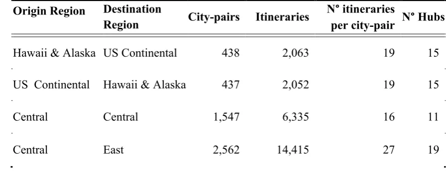
with data not used for the model estimation. Table 2 reports summary statistics for all 267
the entities. The set of hub airports varies between entities, as some hubs do not make 268
sense for some entities for geographical reasons. Table 2 shows the busiest flows in the 269
US ATS network, i.e., the East Coast corridor (East - East entity), the Central corridor 270
(Central – Central entity) and between the Central region and East Coast (Central-East 271
and East-Central entities). A total of 17,200 city-pairs and 104,806 itineraries within the 272
US ATS network are accounted for in the development of the air itinerary share models. 273
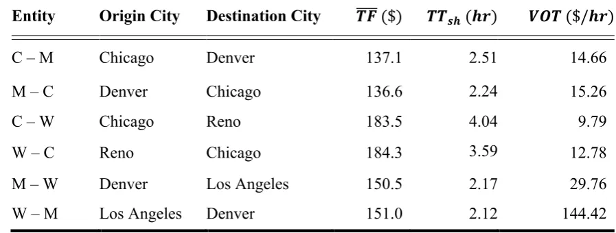
To better understand the results obtained from the air itinerary share model, 274
indicators such as passenegers’ ‘willingness to pay’ can be computed. Value of time 275
(VOT) is the willingness of passengers to pay for one hour of travel and is defined by 276
Eq. (4), which is computed for each given itinerary i. Note that because Travel Fare
277
Ratio is a function of the average air fare in the market and Travel Time Ratio is a 278
13
Vi, average air fare (𝑇𝐹) and minimum flight time (TTsh) are also included in the
280
formulation of VOT. 281
𝑉𝑂𝑇! = !!! !!"#$!
!!! !!"#$%! =
!!"#$!!"#$%&'!#( !!"#$%#&'%(") ∙
!"
!!!! (4)
282
[Table 2] 283
284
Once the itinerary choice model is estimated using the MNL function, Eq. (1) is 285
applied to compute the market share of passengers on each itinerary. The estimated 286
passenger demand per itinerary is then used to compute segment demand – i.e., 287
passenger demand per airport-pair – which will ultimately be used as an input for stage 288
3 of the 3-stage model described in §2, as described in detail by Busquets et al. (2015). 289
4. Application
290
The models described above are applied to a network of 337 airports within the US 291
ATS, as used in the Aviation Integrated Modelling (AIM) Project (2006). The choice of 292
the US air transport network is motivated by improving the current FAA's forecasting 293
methodology, and by the availability of data. The availability of data for the analysis of 294
air transport systems can be challenging, with the US being one of the few countries to 295
provide open source data. 296
The RP data used for this study includes passenger demand data and airfares 297
extracted from the Airline Origin and Destination Survey (DB1B) (BTS-RITA, 2003-298
2010), which contains a 10% sample of airline tickets from reporting carriers. Travel 299
times and costs are also extracted from BTS-RITA (2003-2010). The air itinerary choice 300
14 obtained from the FAA Aviation System Performance Metrics (ASPM) database (FAA, 302
2007-2010). 303
The RP data considered for estimating the model is from 2007, to be in line with 304
the period considered when estimating the ultimate 3-stage model described by 305
Busquets et al. (2015). The data used to validate the model is from 2010. 306
Once the model is estimated, it will be applied in future work to estimate the 307
itinerary shares in the same network of 337 airports into the future. These results will 308
then be compared to those of the Terminal Area Forecasts (TAF) produced by the FAA. 309
5. Model Estimation Results
310
Parameter estimates for the six air itinerary share models mentioned above are reported 311
in Table 3 below. From the entities shown, parameters for the C-W and W-C entities are 312
estimated using 10 different folds of 100 randomly selected city-pairs. The estimated 313
coefficients are averaged to define the final model coefficients. For the C-M, C, M-314
W and W-M entities, the entire estimation dataset is used to estimate the air itinerary 315
share model. As Table 2 shows, the C-W and W-C entities have 724 city-pairs and just 316
over 5,200 itineraries, while the rest of the entities' datasets reported in this paper 317
contain a much lower number of city-pairs and itineraries, making the estimation 318
process less computationally intensive. 319
Model performance is described using the likelihood ratio test and rho-squared 320
parameter (ρ2). The likelihood ratio test provides an evaluation of the entire estimated 321
model by evaluating whether it is possible to reject the null hypothesis that a more 322
restricted model (i.e., a model with zero coefficients) is equal to the estimated one. The 323
15 All estimated coefficients are statistically significant at the 95th percentile
325
confidence level. 326
The Travel Fare Ratio and Travel Time Ratio coefficients are both of the 327
expected sign, negative, indicating that fares and travel time are a resistance to travel. In 328
contrast, some of the coefficients associated with delay at the origin and destination 329
airports are positive, suggesting a correlation between delay and itinerary attractiveness, 330
which is unexpected. For entities C-M, M-C, M-W and W-M, the sign of the 331
coefficients alternates between positive and negative, indicating a positive correlation 332
between delay and itinerary attractiveness associated with Mountain (M) airports. For 333
the C-W and W-C entities both delay parameters are positive. These results may be an 334
indication of airport importance since larger and/or hub airports are expected to have 335
more passengers and flights, and therefore higher delay. This suggests that passengers 336
are more inclined to travel to and from large airports, which is likely because of the 337
increased number of routing alternatives available at these airports. 338
The coefficients associated with airport accessibility are also positive, with the 339
exception of the AccessDEmas coeffient for the C-M entity and the AccessORmas
340
coeffient for the W-C entity. This is opposite to what one would expect since an 341
increased travel time to/from an airport is a resistance to air travel, and given the 342
influence on door-to-door travel time, a negative sign would be expected. However, the 343
coefficients associated with all airport accessibility time variables are small, - with the 344
exception ofthe AccessORmas coefficients for the M-C and M-W entities -, indicating 345
low influence of passenger preferences on itinerary choice. 346
[Table 3] 347
16 The estimated Airline Ratio coefficients tend to be in the order of 10e-2 and 349
positive - with the exception of the coefficient associated with the C-W entity -, 350
indicating low influence of passenger preference on itinerary choice. Coefficients 351
associated with level of service are represented by dummy variables in the models and 352
are characteristics of every entity. These variables show the passengers preference in 353
terms of level of service and connecting hub choice. Due to the fact that each entity has 354
a specific set of hubs and different assumptions have been made in building the 355
connection alternatives, a comparison of the estimated coefficients across entities is not 356
possible. 357
For the variables associated with origin and destination hub information (1hub
358
and no_hub), both coefficients are generally negative, except for the C-W and W-C 359
entities. One would expect a negative correlation between itinerary attractiveness and 360
traveling from or to a hub airport (i.e., 1hub=1), and also between itinerary 361
attractiveness and travelling from and to a non-hub airport (i.e., no_hub=1). In both 362
cases fewer alternatives would exist than for an itinerary between two hubs. The 363
positive correlation for entities C-W and W-C may be because these sets of variables 364
interact only with itineraries belonging to markets in which non-stop options exist, and 365
itineraries from or/and to a non-hub airport may be associated with lower delay as well 366
as lower travel fare ratio than itineraries from and to a hub. 367
Regarding the model performance, both the likelihood ratio test and rho-squared 368
parameters for the six entities show reasonable goodness of fit. Although all the models 369
show a likelihood ratio test large enough to reject the null hypothesis that all 370
coefficients are equal to zero; rho-squared values tend to be largest for those models for 371
which the entire dataset has been used during estimation. While the C-M, M-C, C-W 372
17 C-W and W-C entities are lower than 0.6. The same trend is found for the other air 374
itinerary models estimated. 375
To further analyze the results and understand the effect that the level of service 376
has on the willingness to pay, VOT is computed – using Eq. (4) – for an example case. 377
Table 4 shows the VOT values for the six air itinerary share models presented in this 378
paper. For each of the entities an example case has been chosen and the corresponding 379
VOT value has been computed. Considering that VOT values in the literature are 380
typically under $100/hour (Hsiao & Hansen, 2011; Atasoy & Bierlaire, 2012) several 381
observations can be highlighted from the results presented in Table 4. While the 382
estimated VOT for the specified city-pair belonging to the W-M entity is high compared 383
to the literature (i.e., $144.42/hr), the estimated values for the case examples from the 384
other entities are well below $100/hr, and therefore comparable to those found in the 385
literature. This may be because of a lack of differentiation between fare classes, the 386
level of aggregation of the data used or the differences between the entities’ estimation 387
datasets. 388
[Table 4] 389
6. Model Results Validation
390
The estimated air itinerary share models are validated using data associated with city-391
pairs existing in the corresponding entity for the first quarter of 2010. To evaluate the 392
performance of the model, the market share by itinerary predicted by the model is 393
compared to the observed market share obtained directly from the DB1B dataset (BTS-394
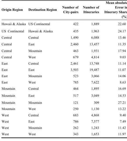
RITA, 2003-2010). Absolute errors are averaged across itineraries, shown in Table 5. 395
Validation results obtained show an average mean absolute error, expressed in terms of 396
18 M-M entity. Most of the percentage errors in itinerary share are lower than those in the 398
literature (e.g., the model developed by Coldren et al. (2003) for 2010 passenger 399
itinerary shares has a mean absolute error of 16.6%). Only the percentage errors 400
accoriated with the M-M entity, the Hawaii & Alaska-US Continental entity and US 401
Continental-Hawaii & Alaska entity are larger. The model specifications and data 402
aggregation, however, differ markedly, so such a direct comparison of model 403
performance is difficult. 404
It is believed that the primary differences lie in the fact of the estimation dataset 405
used to estimate the M-M air itinerary share model has the smallest number of 406
observations compared to the other entities, as shown in Table 2. The high mean 407
absolute error values obtained for the Hawaii & Alaska-US Continental entity and the 408
US Continental-Hawaii & Alaska entity, may be due to the different assumptions 409
implicit in the datasets. While the rest of the entities contain city-pairs with the same 410
time-zone difference, these two entities contain a variety of time zones, which may 411
affect the estimation results. 412
[Table 5.] 413
7. Conclusion and Future Work
414
In this paper a step is made to improve on existing air traffic forecasting methodologies 415
through a better understanding of the factors driving demand, supply and network 416
dynamics. In order to achieve this, an aggregate air itinerary share model is presented 417
that only uses aggregate data, without further insight into service preferences, in 418
contrast to other models in the literature. Given this aggragate input data, the developed 419
model attempts to model demand effects and passenger travel decision more accurately 420
19 for air traffic forecasting, better predictions of airport-pair traffic flows are expected. 422
An aggregate multinomial logit model is estimated to predict how market 423
demand is distributed across available itineraries. In an attempt to capture similarities 424
between city-pairs, eighteen models are developed, each modelling traffic-flow between 425
two major regions of the US ATS. In this paper, results for six entities are presented (C-426
M, M-C, C-W, W-C, M-W and W-M entities). Due to computational limitations some 427
of the models are estimated using a reduced dataset containing information about 100 428
city-pairs in each of 10 runs. Results obtained from the estimated model show high 429
goodness of fit. All estimated coefficients are significant at the 95th percentile 430
confidence level and are generally of the expected sign. 431
The estimated models are validated by computing the mean absolute error 432
between the predicted market share and the observed market share. Data for city-pairs 433
from the 1st quarter of 2010 is used for validation. Validation results show an average 434
mean absolute error of 14.2%, ranging from 7.5% for the W-E entity to 27.2% for the 435
M-M entity. In general, the validation results obtained are slightly better than 436
comparable numbers in the literature (Coldren et al., 2003). However, because of 437
differences in model specifications and data aggregation, a direct comparison is 438
difficult. Model evaluation parameters including likelihood ratio test and Rho-squared 439
show reasonable values, with the likelihood ratio test values large enough to reject the 440
null hypothesis and the Rho-squared values showing a reasonable goodness of fit. 441
Estimated VOTs are found to be in line with those in the literature for all the entities, - 442
i.e. under $100/hr -, with the exception of VOT for the W-M entity. This may be 443
because of a lack of differentiation between fare classes, the level of aggregation of the 444
20 Model estimation results obtained to date look promising, showing that the 446
application of multinomial logit modelling for air itinerary share estimation at the 447
aggregate level is possible. However, computational intensity is a significant problem, 448
requiring the approach to be adjusted to estimate the model with reduced datasets of 100 449
city-pairs in each of 10 runs. This leads to some issues with the estimated coefficients, 450
and may reduce model performance. Hence, further work will focus on improving 451
model estimation results through the use of alternative techniques. Those under 452
consideration include neural networks using various learning algorithms such as 453
backpropagation and Levenberg-Marquardt. 454
In future work the best performing model will be used to estimate the air 455
itinerary shares between city-pairs, so that passenger demand by airport-pair can be 456
predicted and ultimately used as one of the input variables for the final stage of the 3-457
stage model. Additionally, by providing more accurate itinerary shares, this model 458
could be used to aid the decision making process across multiple stakeholders (e.g. 459
airlines, airport providers, government’ agencies, etc.). Route network expansion, 460
equipment purchase or airport expansion are some examples in which its application 461
could be beneficial. Moreover, subject to adequate model refinement, there is the 462
potential of a broader model application to include other transport modes as one of the 463
choice criteria. This would allow for the analysis of, e.g., competition between air and 464
ground transport over short distances. 465
Acknowledgements
466
The authors would like to gratefully acknowledge Dr. Lynnette M. Dray from University
467
College London, Dr. Bilge Atasoy from Massachusetts Institute of Technology and Dr. Gregory
468
Coldren from Coldren Choice Consulting Ltd. for their advice on data sources and approach.
21
Tables
470
Table 1. Input variables considered to influence air itinerary market share. 471
Variable Name Description
Level of service LoS Dummy variable indicating the level of service of the
itinerary i (non-stop or one-stop) with respect the best
level of service within its market (either non-stop or
one-stop with the best connection).
Travel Time Ratio 𝑇𝑇!!"#$% Ratio between travel time of itinerary i and travel time
of shortest itinerary in the market sh.
Travel Fare Ratio 𝑇𝐹!!"#$% Average fare paid on a specific itinerary i divided by
the market average fare.
Multi-airport
system (MAS)
Origin
𝑚𝑎𝑠𝑂𝑅𝐼𝐺! Dummy variable indicating whether the Origin airport
is within a multi-airport systemor not.
Multi-airport
system (MAS)
Destination
𝑚𝑎𝑠𝐷𝐸𝑆𝑇! Dummy variable indicating whether the Destination
airport is within a multi-airport system or not.
Origin airport
average delay
Dly!"#$ Average departure delay of origin airport for the
previous year.
Destination airport
average delay
Dly!"#$ Average arrival delay of destination airport for the
previous year.
22 Accessibility airport.
Destination airport
Accessibility
𝐴𝑐𝑐𝑒𝑠𝑠!"#$ Average distance between city center and destination
airport.
Origin and
destination
airports are hubs
ℎ𝑢𝑏2ℎ𝑢𝑏! Dummy variable indicating whether itinerary i is
between two hub airports.
Either the origin
or destination
airport is a hub
1ℎ𝑢𝑏! Dummy variable indicating whether itinerary i is from
or to a hub airport.
Neither origin nor
destination
airports are a hub
𝑛𝑜_ℎ𝑢𝑏! Dummy variable indicating whether itinerary i is not
from nor to a hub airport.
Airlines Ratio 𝐴𝑖𝑟𝑙𝑖𝑛𝑒𝑠𝑅𝑎𝑡𝑖𝑜! Ratio between the number of airlines serving itinerary
i and the number of airlines serving the shortest
itinerary sh.
[image:23.595.74.522.592.767.2]472
Table 2. Summary statistics for all entities. 473
Origin Region Destination
Region City-pairs Itineraries
N° itineraries
per city-pair N° Hubs
Hawaii & Alaska US Continental 438 2,063 19 15 US Continental Hawaii & Alaska 437 2,052 19 15
Central Central 1,547 6,335 16 11
23
Central Mountain 462 1,867 17 17
Central West 724 5,216 38 19
East Central 2,552 15,150 38 18
East East 3,520 21,157 27 17
East Mountain 508 2,895 18 20
East West 867 9,268 87 24
Mountain Central 463 1,899 15 18
Mountain East 527 3,150 24 18
Mountain Mountain 134 359 5 6
Mountain West 252 1,230 27 11
West Central 724 5,222 38 19
West East 862 9,274 90 24
West Mountain 265 1,313 29 11
West West 356 1,941 31 9
Total 17,200 104,806
[image:24.595.76.526.65.574.2]474
Table 3. Estimated coefficients for the air itinerary choice model corresponding to 475
entities C-M, M-C, C-W, W-C, M-W and W-M. 476
Variable Name C – M M – C C – W W – C M – W W - M
Level of Service
(relevant to every entity) -- -- -- -- -- -- Markets Containing
24
hub2hub 0.000 0.000 0.000 0.000 0.000 0.000
1hub -1.590 -2.090 0.013 0.626 -1.090 -0.846
no_hub -1.410 -2.650 0.095 0.928 -1.970 -1.380
Airlines Ratio 0.012 0.017 -0.550 0.017 0.010 0.023
Travel Fare Ratio (TFRatio) -3.840 -4.080 -0.789 -1.321 -1.970 -0.754
Travel Time Ratio (TTRatio) -1.030 -1.020 -0.170 -0.329 -0.844 -1.530
𝐷𝑙𝑦!"#$ -0.174 3.950 0.086 0.627 2.010 -0.026
𝐷𝑙𝑦!"#$ 2.930 -0.092 0.542 0.227 -0.067 1.110
AccessDEmas -0.919 0.020 0.044 0.015 0.002 0.331
AccessORmas 0.098 0.864 0.098 -0.001 0.749 0.005
LogLikelihood Ratio Test 523,121 435,323 1,030,223 191,252 908,296 906,390
Rho-squared (ρ2) 0.724 0.691 0.587 0.559 0.715 0.714
*Note: All variables are statistically significant at the 95% confidence level.
[image:25.595.77.526.564.734.2]477
Table 4. Comparison between Value of Time for the C-M, M-C, C-W, W-C, M-W and 478
W-M entities. 479
Entity Origin City Destination City 𝑻𝑭 ($) 𝑻𝑻𝒔𝒉(𝒉𝒓) 𝑽𝑶𝑻 ($/𝒉𝒓)
C – M Chicago Denver 137.1 2.51 14.66
M – C Denver Chicago 136.6 2.24 15.26
C – W Chicago Reno 183.5 4.04 9.79
W – C Reno Chicago 184.3 3.59 12.78
M – W Denver Los Angeles 150.5 2.17 29.76 W – M Los Angeles Denver 151.0 2.12 144.42
25 Table 5. Mean absolute error in itinerary share computed in terms of percentage
481
deviation. 482
Origin Region Destination Region Number of
City-pairs
Number of Itineraries
Mean absolute Error in Itinerary Share (%)
Hawaii & Alaska US Continental 422 1,889 22.60
US Continental Hawaii & Alaska 435 1,963 24.17
Central Central 1,490 6,088 13.46
Central East 2,460 13,457 11.35
Central Mountain 463 1,931 17.94
Central West 679 4,814 9.03
East Central 2,461 13,748 11.14
East East 3,503 19,487 11.07
East Mountain 523 3,066 14.06
East West 785 7,622 8.63
Mountain Central 464 1,895 16.69
Mountain East 517 3,049 14.53
Mountain Mountain 121 309 27.21
Mountain West 250 1,130 13.22
West Central 683 4,868 9.40
West East 786 7,577 7.49
West Mountain 262 1,243 11.42
West West 343 1,653 11.97
483
484
References
485 486
Adler, N. (2001). Competition in a deregulated air transportation market. European
487
26 AIM. (2006). Aviation Integrated Modelling Project. Retrieved August 15, 2016, from 489
Aviation Integrated Modelling Project: http://www.aimproject.aero/. 490
Atasoy, B., & Bierlaire, M. (2012). An itinerary choice model based on a mixed RP/SP
491
dataset. ENAC, EPFL. Lausanne: Transport and Mobility Laboratory, ENAC. 492
Bierlaire, M. (2003). Biogeme: A free package for the estimation of discrete choice 493
models. 3rd Swiss Transportation research conference. Ascona, Switzerland. 494
Retrieved from Biogeme: A free package for the estimation of discrete choice 495
models. 496
BTS-RITA. (2003-2010). Bureau of Transportation Statistics - Research and
497
Innovative Technology Administration. Retrieved September 14, 2014, from 498
Origin and Destination Survey: DB1B Market for 1003 to 2007: 499
http://www.transtats.bts.gov/DL_SelectFields.asp?Table_ID=247&DB_Short_N 500
ame=Origin%20and%20Destination%20Survey 501
Busquets, J. G., Alonso, E., & Evans, A. D. (2015). Application of Data Mining in Air 502
Traffic Forecasting. AIAA Aviation Technology, integration and Operations
503
Conference. Dallas: AIAA. 504
Busquets, J. G., Alonso, E., & Evans, A. D. (2016). Predicting Aggregate Air Itinerary 505
Shares Using Discrete Choice Modeling. AIAA, Aviation Technology,
506
Integration and Operations Conference. Washington D.C. 507
Carrier, E. (2008). Modeling the Choice of an Airline Itinerary and Fare Product using
508
booking and Seat Avaiability Data. Cambridge, Massachusetts: Massachusetts 509
Institute of Technology. 510
Coldren, G. M., & Koppelman, F. S. (2005). Modeling the competition among air-travel 511
itinerary shares. GEV model development. Transportation Research Part A:
512
27 Coldren, G. M., Koppelman, F. S., Kasturirangan, K., & Mukherjee, A. (2003).
514
Modeling aggregate air travel itinerary shares: logit model development at a 515
major US airline. Journal of Air Transport Management, 9(6), 361-369. 516
FAA. (2007-2010). Federal Aviation Administration. Retrieved September 20, 2015, 517
from FAA Operations & Performance Data: https://aspm.faa.gov 518
FAA. (2014). Federal Aviation Administration. Retrieved October 10, 2015, from 519
Aviation System Performance Metrics (ASPM) Manuals: https://aspm.faa.gov/ 520
Garrow, L. A. (2010). Discrete Choice Modelling And Air Travel Demand: theory.
521
Aldershot, United Kingdom: Ahsgate. 522
Gramming, J., Hujer, R., & Scheidler, M. (2005). Discrete choice modelling in airline 523
network management. Journal of Applied Economics, 20, 467-486. 524
Grosche, T., & Rothlauf, F. (2007). Air Travel Itinerary Market Share Estimation.
525
Manheim: University of Manheim. 526
Hansen, M. (1995). Positive feedback model of multiple-airport system. ASCE Journal
527
of Transportation Engineering, 121 (6), 453-460. 528
Hsiao, C., & Hansen, M. (2011). A passanger demand model for air transportation in a 529
hub-and-spoke network. Transportation Research Part E: Logistics and
530
Transportation Review(47), 1112-1125. 531
Kotegawa, T. (2012). Analyzing the evolutionary mechanism of the air transportation
532
system-of-system using network theory and machine learning algorithm. West 533
Lafayette, Indiana: Faculty of Purdue University. 534
Louviere, J. J., Meyer, R. J., Bunch, D. S., Carson, R., & Dellaert, B. (1999). Combinig 535
sources of preference data for modeling complex decision provesses. Marketting
536
28 Proussaloglou, K., & Koppelman, F. S. (1995). Air carrier demand: an analysis of 538
maket share determinants. Transportation, 22(4), 371-388. 539
Warburg, V., Bhat, C., & Adler, T. (2006). Modeling demographic and unobserved 540
heterogeneity in air passengers' sensitivity to service attributes in itinerary 541
choice. Transportation Research Record: Journal of the Transportation
542
Research Board, 1951, 7-16. 543
Windle, R., & Dreesner, M. (1995). Airport Choice in multiple-aiport regions. ASCE
544
Journal of Transportation Engineering, 121(4), 332-337. 545
546