doi:10.1093/imanum/dry007
Numerical methods for changing type systems
Sebastian Franz∗
Institute of Scientific Computing, Technische Universität Dresden, 01062 Dresden, Germany ∗Corresponding author: [email protected]
Sascha Trostorff
Institute of Analysis, Technische Universität Dresden, 01062 Dresden, Germany
and Marcus Waurick
Department of Mathematics, University of Strathclyde, Glasgow, UK
[Received on 01 August 2017; revised on 13 December 2017]
In this paper we develop a numerical method for partial differential equations with changing type. Our method is based on a unified solution theory found by Rainer Picard for several linear equations from mathematical physics. Parallel to the solution theory already developed, we frame our numerical method in a discontinuous Galerkin approach in time with certain exponentially weighted spaces combined with a finite element method in space.
Keywords: evolutionary equations; changing type system; discontinuous Galerkin; space-time approach.
1. Introduction
Following the rationale presented in the study by (Picard, 2009), most of the classical linear partial differential equations arising in mathematical physics share a common form, namely the form of an evolutionary problem. That is, we consider equations of the form
(∂tM0+M1+A)U=F, (1.1)
whereF is a given source term,∂tstands for the derivative with respect to time,M0,M1are bounded
linear operators on some Hilbert spaceHandAis an unbounded skew-selfadjoint operator inH, which we shall identify with their canonical extensions toH-valued functions acting as abstract multiplication operators. We are seeking for a unique solutionU of the above equation. We remark here that we do not impose initial conditions, since we consider the whole real line as time horizon, and hence, we implicitly assume a vanishing initial value at ‘−∞’. To illustrate the setting, we begin with presenting some examples.
Example1.1 LetΩ ⊆Rnan open nonempty set, wheren∈N, but, typicallyn∈ {1, 2, 3}. We define
the following two differential operators
assigning each functionu ∈ H01(Ω)its gradient, that is, the column vector of its partial derivatives in each coordinate direction. Moreover, we set
div := −(∇0)∗:D(div)⊆L2(Ω)n→L2(Ω),
which is nothing but the operator assigning each L2 vector field its distributional divergence with maximal domain, that is,
D(div)=
v∈L2(Ω)n :
n
i=1
∂ivi∈L2(Ω)
.
Since both the operators ∇0 and div are closed and skew adjoints of one another, we infer that the
operator
A:=
0 div ∇0 0
:D(∇0)×D(div)⊆L2(Ω)×L2(Ω)n→L2(Ω)×L2(Ω)n
is skew selfadjoint on the Hilbert spaceH=L2(Ω)×L2(Ω)n. ChoosingM0=1 00 1andM1=0 00 0
in (1.1), the corresponding evolutionary problem reads as
∂t 1 0 0 1 + 0 div ∇0 0
u v = f g .
Ifg=0, this is nothing but the wave equation. Indeed, the second line then gives∂tv= −∇0u, and
hence, differentiating the first line with respect to time, we obtain
∂t2u−div∇0u=∂ttu+div∂tv=∂tf.
Note that div∇0=ΔDis the classical Dirichlet–Laplace operator onL2(Ω).
ChoosingM0= 1 0
0 0
andM1= 0 0
0 1
in (1.1), the corresponding problem reads as
∂t 1 0 0 0 + 0 0 0 1 + 0 div ∇0 0
u v = f g .
Setting againg=0, the latter gives the heat equation. Indeed, the second line readsv= −∇0uand hence
the first line yields
Finally, choosingM0= 0 0
0 0
andM1= 1 0
0 1
in (1.1), we get
1 0 0 1
+
0 div ∇0 0
u v
=
f g
,
which in the caseg=0 gives the elliptic equation
u−div∇0u=f.
Remark1.2 Note that we can treat the case of homogeneous Neumann boundary conditions in the same way. The only difference is that we define∇ as the distributional gradient onH1(Ω) and div0:= −(∇)∗. Replacing now∇0by∇ and div by div0yields the same hyperbolic, parabolic and elliptic type
problem above, but now with homogeneous Neumann boundary conditions.
Example1.1shows that evolutionary problems cover all three classical types of partial differential equations, elliptic, parabolic and hyperbolic. However, also, problems of mixed type are covered as the next example shows.
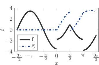
Example1.3 Recall the setting of Example1.1. We decomposeΩ into three measurable, disjoint sets
Ωell,ΩparandΩhypand setM0=
χΩhyp∪Ωpar 0 0 χΩhyp
as well asM1=
χΩell 0
0 χΩpar∪Ωell
. The resulting
evolutionary problem then is of mixed type. More precisely, onΩellwe get an equation of elliptic type,
onΩparthe equations becomes parabolic while onΩhypthe problem is hyperbolic.
Remark1.4 The interested reader might wonder that there is no transmission condition imposed on the unknown quantities along the interfaces ofΩell,ΩparandΩhyp. However, this can be implemented
automatically by being in the domain of the corresponding operator sum, as can be seen, for instance, in the study by (Waurick, 2016, Remark 3.2), see also the study by (Picardet al., 2013, An illustrative Example). Another example of a mixed type problem in control theory can be found in the study by (Picardet al., 2016, Remark 6.2).
In the study by (Picard, 2009), the well-posedness of problems of the form (1.1) has been addressed. In fact, it was shown that these problems also cover the classical Maxwell’s equations, the equations of linearized elasticity or a general class of coupled phenomena, see, for instance, the studies by (Mukhopadhyay et al., 2015; Picard et al., 2015; Mulholland et al., 2016). All these problems are indeed well-posed (see Section2 for the precise statement). The purpose of the present article is to provide numerical methods for such problems. In this article, for the applications to follow, we will focus, however, on problems of mixed type of the form sketched in Example1.3. Moreover, as the spatial discretization has to be developed for each problem separately, anyway, in this work, we will put an emphasis on the time discretization. Furthermore, we want to stress that the null space ofM0in
(1.1) might be infinite-dimensional. Hence, we seek to develop a numerical scheme, which in particular allows for the treatment of a certain class of (partial) differential-algebraicequations.
A similar approach for a unified treatment of elliptic and hyperbolic problems was already suggested by Friedrichs in 1958, see the study by (Friedrichs, 1958), where both types of problems are written as an abstract operator equationKu=f with an accretive symmetric operatorK. These equations are known
local operators in space are considered. Nonstationary examples of mixed type have, however, not been treated.
A drawback of Friedrichs systems is that they ignore the particular role of time in the way that they do not distinguish between the time coordinate and the spatial coordinates. Therefore, the characteristic property of time evolution, namely causality, is not considered at all. In contrast, the systems considered here are automatically causal in direction of time due to a uniform positive definiteness constraint on the operators involved (compare Remark2.3).
Based on the framework of Friedrichs systems, a unified numerical treatment of different types of partial differential equations, also including certain equations of changing type, was studied before. We refer to the articles by (Ern & Guermond, 2006a,2006b,2008) and to the Ph.D. thesis by (Jensen, 2004). We emphasize that our approach covers problems with change of type ranging from elliptic to hyperbolic but also to parabolic type problems on different spatial domains. In this sense, we obtain a natural unified treatment of a class of partial differential equations that might go beyond the consideration of Friedrichs systems. Note that in a very rough comparison the above mentioned operator
Kis not symmetric in our situation. In particular, the operator equations considered also cover Maxwell’s
equations with eddy current approximation on parts of the underlying domain.
For the numerical treatment of the time derivatives we use a discontinuous Galerkin (dG) method, see also Section3. The first dG method was published in 1973 on neutron transport (Reed & Hill, 1973). Later the methodology was developed further for classical hyperbolic, parabolic and elliptic problems, see also the survey article by (Cockburnet al., 2000) and the book by (Rivière, 2008). Note that there is a strong connection between dG methods and Runge–Kutta (collocation) methods, see the study by (Akriviset al., 2011) for parabolic problems.
In Section2, for convenience, we will recall some essentials for evolutionary equations. In particular, we recall the solution theory of problems of the type of equation (1.1). We will introduce a semidiscretized version, Equation (3.1), of Equation (1.1) at the beginning of Section3. We will also provide a solution theory for this semidiscretized variant with general underlying (spatial) Hilbert space
H(Proposition3.2). The remainder of Section3is devoted to estimate difference of the exact solution of (1.1) and the approximate solution of (3.1). In Subsection3.1, we bound the error by solely in terms of the interpolation error, which will eventually be estimated in Subsection3.2. As our prime example, we address the full space-time discretization of Example1.3and derive corresponding error estimates. We verify our theoretical findings in Section5by means of a 1 + 1- and a 1 + 2-dimensional numerical example.
In general, we identify functions defined on a subset ofRwith their extension toRby 0.
2. The setting of evolutionary problems
In this section we briefly recall the well-posedness result stated in the study by (Picard, 2009). For doing so, we need to specify the functional analytic setting. Throughout, letHbe a real Hilbert space. Definition2.1 Letρ >0 and define the space
Hρ(R;H):=
⎧ ⎨
⎩f :R→H;f meas.,
R
|f(t)|2Hexp(−2ρt)dt<∞
⎫ ⎬ ⎭,
where we as usual identify functions which are equal almost everywhere. The space Hρ(R;H)is a Hilbert space endowed with the natural inner product given by
f,gρ :=
R
Moreover, we define∂tto be the closure of the operator
∂t :C∞c (R;H)⊆Hρ(R;H)→Hρ(R;H):ϕ→ϕ′,
where by C∞c (R;H)we denote the space of infinitely differentiable H-valued functions on Rwith compact support. We denote the domain of∂tkbyHρk(R;H)fork∈N.
Within the setting introduced, we can formulate the well-posedness for evolutionary equations of the form (1.1).
Theorem2.2 (Picard, 2009, Solution Theory) LetM0,M1:H→Hbe bounded linear operators,M0
selfadjoint andA:D(A)⊆H→Hskew selfadjoint. Moreover, assume that there is someρ0>0 such
that
∃γ >0∀ρρ0,x∈H: (ρM0+M1)x,xH γ x,xH.
Then, for eachρρ0and eachF∈Hρ(R;H)there exists a uniqueU∈Hρ(R;H)such that
(∂tM0+M1+A)U=F, (2.1)
where the closure is taken inHρ(R;H). Moreover, the following continuity estimate holds
|U|ρ 1
γ|F|ρ.
IfF∈Hρk(R;H)fork∈N, then so isUand we can omit the closure bar in (2.1). Remark2.3
(a) Note that the positive definiteness condition in the latter theorem especially implies
M0x,xH 0 for eachx∈H.
(b) We remark thatHρ1(R;H) ֒→Cρ(R;H)by a variant of the Sobolev embedding theorem (Picard
& McGhee, 2011, Lemma 3.1.59) or (Kalauchet al., 2014, Lemma 5.2). Here,
Cρ(R;H):=
f :R→H; f cont., sup t∈R|
f(t)|exp(−ρt) <∞
.
(c) IfF∈H1ρ(R;H)thenU∈Hρ1(R;H), and hence
AU=F−∂tM0U−M1U∈Hρ(R;H),
which yields that U(t) ∈ D(A) for almost every t ∈ R. If even F,U ∈ Hρ2(R;H) the latter gives AU ∈ Hρ1(R;H) and hence, using the Sobolev embedding result (see part (b)),
U∈Cρ(R;D(A)).
(d) We note that the constantγ in the positive definiteness constraint above is chosen uniformly inρ ρ0. This uniformity yields the causality of the solution operator, see e.g., the study by
(e) The original result in the study by (Picard, 2009) treats a general class of time-translation invariant coefficients. We refer to the studies by (Picard et al., 2013; Waurick, 2015) for nonautonomous variants as well as to the studies by (Trostorff, 2012;Trostorff & Wehowski, 2014) for nonautonomous and/or nonlinear versions of Theorem2.2.
(f) In order to incorporate initial value problems, one extends the solution theory to certain distributional right-hand sides (Picard & McGhee, 2011, Section 6.2.5). Indeed, an initial condition of the formM0U(t0+) =M0x0 for somet0 ∈ R,x0 ∈ Hcan be implemented by
solving the equation
(∂tM0+M1+A)U=F+δt0M0x0
for some F ∈ Hρ(R;H)supported on [t0,∞). Employing causality, one indeed obtains the
solutionU satisfies the asserted initial condition (see again the study by Picard & McGhee, 2011, Section 6.2.5).
We note that the equations treated in Example1.1and Example1.3satisfy the conditions of the previous theorem, and hence are well-posed.
3. Semidiscretization in time
In this section, we discretize (1.1) with respect to time and do thea priorianalysis. We assume thatA,
M0,M1satisfy the assumptions of Theorem2.2. Letρρ0and fixT>0 and consider the time interval
[0,T] instead of the whole real line. We partition the time interval [0,T] into subintervalsIm=(tm−1,tm]
of lengthτmform∈ {1, 2,. . .,M}witht0=0 andtM=T. Letq∈N. We define the space
Vτ := {u∈Hρ(R;H:);∀m∈ {1,. . .,M}:u|Im ∈Pq(Im;H)},
where we denote by
Pq(Im;H):=lin{Im∋t→tkζ ∈H;k∈ {0,. . .,q},ζ ∈H}
the space ofH-valued polynomials of degree at mostqdefined onIm. We endow Pq(Im;H)with the
scalar product
p,qρ,m:= tm
tm−1
p(t),q(t)Hexp(−2ρ(t−tm−1))dt
turning the spacePq(Im;H)into a Hilbert space.
The time integrals have to be evaluated numerically. We choose on each time intervalIm a
right-sided weighted Gauß–Radau quadrature formula. To this end, denote byωmi andˆtmi ,i∈ {0,. . .,q}, the weights and nodes of the weighted Gauß–Radau formula withq+ 1 nodes on the reference time interval
I=(−1, 1], such that
I
e−ρτm(t+1)p(t)dt= q
i=0
ωmi p(ˆtim)
paper (Trostorff & Waurick, 2016) for some basic facts on the Gauß–Radau quadrature. With the standard linear transformationTm :I → Im and the transformed Gauß–Radau pointstm,i := Tm(ˆtmi ),
i∈ {0,. . .,q}, we define by
Qm[v] :=
τm
2
q
i=0
ωmi v(tm,i)
a quadrature formula onIm. Note that for all polynomials of degree at most 2q we haveQm[p] = p, 1ρ,m.
Using
Qm[a,b]ρ:=Qm[a,bH]
instead of the scalar products a,bρwe employ the following discretequadrature formulation: For givenF∈Vτandx0∈H, findUτ ∈Vτ, such that for allΦ ∈Vτandm∈ {1, 2,. . .,M}it holds
Qm(∂tM0+M1+A)Uτ,Φρ+ M0[[Uτ]]xm0−1,Φm+−1H =Qm[F,Φ]ρ. (3.1) Here, we denote by
[[Uτ]]x0 m−1:=
Uτ(tm−1+)−U(tm−1−), m∈ {2,. . .,M}
Uτ(t0+)−x0, m=1,
the jump attm−1and byΦm+−1:=Φ(tm−1+).
Remark3.1 We shall briefly comment on the derivation of (3.1). We start with the formulation of an inital value problem given in Remark2.3(f), i.e., with the equation
(∂tM0+M1+A)U=F+δ0M0x0.
We shall do so for the example caseM=1, i.e., only one interval, first. Testing the latter equation with
Φ∈Vτ we obtain
(∂tM0+M1+A)U,Φρ = F,Φρ+ M0x0,Φ(0+)H.
By a standard penalization technique we impose the initial condition weakly in the following way
(∂tM0+M1+A)U,Φρ+ M0U(0+)−M0x0,Φ(0+)H = F,Φρ.
Using the quadrature formula instead of the inner products, we derive (3.1) form=M=1.
For the general case, we repeat this argument and takeU(tm−1+) as the new initial value and hence
obtain (3.1) for each interval.
Proposition3.2 LetF∈Vτ,x0∈H. Then there exists a unique solution of (3.1).
Proof. Letm∈ {1,. . .,M}and recall thatPq(Im;H)is a Hilbert space with the aforementioned scalar
product. We note that
and
δm−1:Pq(Im;H)→R: p→p(tm−1+)
are bounded linear operators. Consequently, the mapping
Pq(Im;H)→R:p→ x,δm−1pH
is linear and bounded for eachx∈Hand thus, by the Riesz representation theorem, there is a unique
Ψ (x)∈Pq(Im;H)such that
Ψ (x),pρ,m= x,δm−1pH.
Moreover, the mappingΨ :H→Pq(Im;H)is linear and bounded, since
|Ψ (x)|2ρ,m= Ψ (x),Ψ (x)ρ,m= x,δm−1Ψ (x)H |x|Hδm−1|Ψ (x)|ρ,m (x∈H).
We now prove that for eachg∈Pq(Im;H)there is a uniqueu∈Pq(Im;D(A))such that
(∂tM0+M1+A)u+ΨM0δm−1u=g. (3.2)
For doing so, we first compute using integration by parts
∂tM0v,vρ,m=
1
2 ∂tM0v,vρ,m+ 1 2
tm
tm−1
v(t),M0v′(t)Hexp(−2ρ(t−tm−1))dt
= 1
2 ∂tM0v,vρ,m− 1 2
tm
tm−1
M0v′(t),v(t)Hexp(−2ρ(t−tm−1))dt
+ρ
tm
tm−1
M0v(t),v(t)Hexp(−2ρ(t−tm−1))dt+
1
2 M0v(tm),v(tm)Hexp(−2ρτm)
−1
2 M0v(tm−1),v(tm−1)H
ρ M0v,vρ,m−
1
2 ΨM0δm−1v,vρ,m
for eachv∈Pq(Im;H). Next, fromA∗= −Ait follows Ax,xH=0 for eachx∈D(A). Therefore, for
allu∈Pq(Im;D(A)), we get
(∂tM0+M1+A)u+ΨM0δm−1u,uρ,m= ∂tM0u,uρ,m+ M1u,uρ,m+ ΨM0δm−1u,uρ,m (3.3)
(ρM0+M1)u,uρ,m+
1
2 ΨM0δm−1u,uρ,m
where we have used
ΨM0δm−1u,uρ,m= M0u(tm−1+),u(tm−1+)H0.
In particular, bothB:=(∂tM0+ M1) +M0δm−1andB+Aare strictly positive definite. Moreover,
sinceBis bounded,B∗is strictly positive definite, as well. Hence, from
(B+A)∗=B∗−A
we read off that (B+ A)∗is strictly positive definite as well. Thus, for eachg ∈ Pq(Im;H)there is a
uniqueu∈Pq(Im;D(A))=D(A+B)such that
(∂tM0+M1+A)u+ΨM0δm−1u=g. (3.4)
Thus, we are in the position to define a solution for (3.1) by induction onm. For this, we putU(t0−) := x0. Next, assume we have solved (3.1) forUτ onIm−1 for somem∈ {1, . . .,M}(I0:= {t0}and the
equation is void). Then, letu∈Pq(Im;D(A))be such that (3.4) holds forg=F|Im −ΨM0U
τ(t
m−1−).
We putUτ|Im :=u. The thus defined functionU
τ solves (3.1): we observe
(∂tM0+M1+A)Uτ,Φρ,m+ ΨM0δm−1Uτ,Φρ,m
= F−ΨM0Uτ(tm−1−),Φρ,m= F,Φρ,m+ ΨM0Uτ(tm−1−),Φρ,m,
by definition for allΦ ∈Vτandm∈ {1,. . .,M}. The latter is the same as saying
(∂tM0+M1+A)Uτ,Φρ,m+ M0Uτ(tm−1+),Φ(tm−1+)H
= F,Φρ,m+ M0Uτ(tm−1−),Φ(tm−1+)H.
But, since the quadrature is exact for polynomials up to degree 2q, the latter equation in turn is equivalent to
Qm(∂tM0+M1+A)Uτ,Φρ+ M0[[Uτ]]xm0−1,Φm+−1H =Qm[F,Φ]ρ,
which yields existence ofUτ. Uniqueness follows from the uniqueness ofusatisfying (3.4).
Remark 3.3 (Dissipation of energy) To use dG methods for time stepping is known to be slightly dissipative in the following sense. Let us consider the weak formulation of (1.1) withUas test function and time integration over(−∞,T), i.e.,
(∂tM0+M1+A)U,Uρ,(−∞,T)= F,Uρ,(−∞,T).
Assuming a nonzero value ofU(0) and F(t)=0 fort 0, we obtain for eacht >0 the following conservation law of the energy:
For our dG method we obtain in the discrete pointsti>0 the conservation law of the discrete energy
e−2ρti M
0Uτ−i ,Uτ−i H+2 (ρM0+M1)Uτ,Uτρ,(0,ti)
+ i
m=1
e−2ρtm−1 M
0[[Uτ]]xm0−1, [[Uτ]]xm0−1H = M0Uτ0−,Uτ−0H.
From the two conservation laws we observe a reduction of the discrete energy compared to the original energy over time due to the jumps. There are time-stepping methods, using different ansatz and test spaces, without such a dissipation. We will consider them in a future publication. Here we analyse the dissipative dG method because its ansatz and trial spaces are the same. It therefore fits better in the theoretical framework of (Picard, 2009).
Remark 3.4 In the proof of Proposition3.2 the importance of the introduction of the exponential weight—also for the finite time regime—becomes apparent. Indeed, the exponential weight serves to ensure strict positive definiteness of the operator appearing in (3.2) in space time, see also (3.3). If on the other hand one uses an unweightedL2 space in Proposition3.2the same result holds due to the equivalence of the corresponding norms on finite time intervals.
3.1 On some a priori error estimates in time
After having proved the unique solvability of (3.1), we address the error estimates in the following. In our analysis we will use the discretized norms
v2Q,ρ,m:=Qm[v,v]ρ and v2Q,ρ :=
M
m=1
Qm[v,v]ρe−2ρtm−1
as approximations ofv2ρ,m := Im|v(t)| 2
Hexp(−2ρ(t−tm−1))dtand|v|2ρ. Note that forv∈ Vτ the approximation is exact.
Let us start by defining an interpolation operator intoVτ and define byϕ
m,iwithi∈ {0,. . .,q}the
associated Lagrange basis functions to the nodestm,i. Then we obtain for a functionv∈C([0,T],H) by
(Pv)(0)=v(0), (Pv)I
m(t)= q
i=0
v(tm,i)ϕm,i(t), m∈ {1,. . .,M}, (3.5)
an interpolation operator in time.
In the analysis to follow, we will consider the problem (2.1). In particular, we emphasize that we assume that the hypotheses of Theorem2.2 are in effect. Furthermore, we fix a right-hand side
F∈H2ρ(R;H). Thus, by Theorem2.2(and Remark2.3(c)) there exists a unique solution
Also, by Remark2.3(c), we obtainF∈Cρ(R;H)andU∈Cρ(R;D(A))∩C1ρ(R;H). Moreover, we set
Uτ ∈Vτ to satisfy (3.1) for the right-hand sidePF ∈ Vτ andx
0:=U(0+). We consider the following
splitting:
Uτ−U=ξ −η, where ξ =Uτ−PU∈Vτ and η=U−PU.
Note that due to the better regularity ofUmentioned above, the equation holds pointwise, that is, for everyt∈[0,T] we have that
(∂tM0+M1+A)U(t)=F(t)
and thus,
(∂tM0+M1+A)U(t),Φ(t)H = F(t),Φ(t)H
for eachΦ∈Vτ and everyt∈[0,T], which gives
Qm[(∂tM0+M1+A)U,Φ]ρ+ M0[[U]]xm0−1,Φm+−1H =Qm[F,Φ]ρ =Qm[PF,Φ]ρ,
where we have usedM0[[U]]xm0−1 = M0[[U]]Um−(01+) =0, due to the continuity ofU andQm[F,Φ]ρ =
Qm[PF,Φ]ρ, since PF interpolates at the Gauß–Radau points used in the quadrature. Hence, U (formally) solves the same semidiscretized problem asUτ. Thus, we obtain withχ∈Vτ as test function theerror equation
Qm[(∂tM0+M1+A)ξ,χ]ρ+ M0[[ξ]]0m−1,χm+−1H
=Qm[(∂tM0+M1+A)η,χ]ρ+ M0[[η]]0m−1,χm+−1H. (3.7)
For the special caseχ=ξ (useA= −A∗) we obtain
Edm:=Qm[(∂tM0+M1)ξ,ξ]ρ+ M0[[ξ]]0m−1,ξm+−1H
=Qm[(∂tM0+M1+A)η,ξ]ρ+ M0[[η]]0m−1,ξm+−1H =:Emi (3.8)
for allm∈ {1,. . .,M}, where the subscripts d and i should remind of discretization and interpolation, respectively.
Lemma3.5 For allm∈ {1,. . .,M}, we have
Edmγξ2Q,ρ,m+1
2
M0ξm−,ξm−He−2ρτm− M0ξm−−1,ξm−−1H+ M0[[ξ]]0m−1, [[ξ]]0m−1H
,
Proof. Letm∈ {1,. . .,M}. Sinceξis a (piecewise) polynomial of orderqin time, we obtain
Qm[∂tM0ξ,ξ]ρ= ∂tM0ξ,ξρ,m = 1
2
Im
e−2ρ(t−tm−1)∂
t M0ξ,ξHdt = 1
2
M0ξm−,ξm−He−2ρτm− M0ξm+−1,ξm+−1H
+ρ M0ξ,ξρ,m.
Further, we compute
M0[[ξ]]0m−1,ξm+−1H=
1 2
M0ξm+−1,ξm+−1H− M0ξm−−1,ξm−−1H+ M0[[ξ]]m0−1, [[ξ]]0m−1H
.
Therefore, we have
Emd =Qm[(∂tM0+M1)ξ,ξ]ρ+ M0[[ξ]]0m−1,ξm+−1H = 1
2
M0ξm−,ξm−He−2ρτm− M0ξm−−1,ξm−−1H+ M0[[ξ]]0m−1, [[ξ]]0m−1H
+ (ρM0+M1)ξ,ξρ,m.
Together with
(ρM0+M1)ξ,ξρ,mγξ2ρ,m =γξ
2 Q,ρ,m
the lemma is proved.
In order to analyseEimwe introduce another interpolation operator that enables us to estimate the time derivative of the interpolation error with a higher order. This operator utilizestm,−1:=tm−1 in
addition totm,i,i∈ {0,. . .,q}as interpolation points. Denoting the associated Lagrange basis functions
byψm,i,i∈ {−1, 0,. . .,q}, this interpolation operator is given by
(Pv)I
m(t):= q
i=−1
v(tm,i)ψm,i(t), m∈ {1,. . .,M}. (3.9)
Note thePmaps to functions that are continuous in time (recall thattm,q=tm) while the image ofPis
allowed to be discontinuous at the time mesh points.
Lemma3.6 Form∈ {1,. . .,M}andψ∈Vτ, we have
Qm[∂tM0η,ψ]ρ+ M0[[η]]0m−1,ψm+−1H =Qm
∂tM0(U−PU),ψ
ρ+R(U,ψ ), where
|R(U,ψ )|Cατm|M0ηm+−1|2H+βψ2Q,ρ,m
Proof. With U being continuous in time, we only have to consider the discrete part. Using the exactness of the quadrature rule for polynomials of degree 2qand integration by parts, we obtain for
m∈ {1,. . .,M}
Qm[∂tM0PU,ψ]ρ+ M0[[PU]]xm0−1,ψm+−1H
=:a
= ∂tM0PU,ψρ,m+a
= − M0PU,∂tψρ,m+2ρ M0PU,ψρ,m+ e−2ρ(t−tm−1)M0PU,ψH tm
tm−1
=:b
+a
= − Qm[M0PU,∂tψ]ρ
=Qm
M0PU,∂tψ
ρ= M0PU,∂tψρ,m
+2ρ M0PU,ψρ,m+a+b
= ∂tM0PU,ψρ,m+2ρ(M0PU,ψρ,m− M0PU,ψρ,m)+a+b− e−2ρ(t−tm−1)M0PU,ψH tm
tm−1
=:c
.
Using(PU)−m−1=(PU)+m−1(m2),(PU)0+=U(0+)=x0and(PU)−m =(PU)−m(m1), we have a+b−c=0.
Furthermore, it holds
2ρ( M0PU,ψρ,m− M0PU,ψρ,m)=2ρ M0((P−P)U)(tm+−1)χ,ψρ,m
=2ρ M0(PU−U)(tm+−1)χ,ψρ,m=:R(U,ψ ),
whereχ ∈Pq+1(Im)withχ(tm−1)=1 andχ(tm,i)=0,i∈ {0,. . .,q}. By (Trostorff & Waurick, 2016,
Corollary 1.4) forK=T (note that 0 < τm = |Im|T), we obtainχ2ρ,m Cτmfor someC 0.
Thus, we get
|R(U,ψ )|2ρM0(PU−U)(t+m−1)Hχρ,mψρ,m
C2(2ρ)2ατm|M0(PU−U)(t+m−1)|2+βψ2Q,ρ,m,
whereαβ=1/4. Combining above transformations we are done.
Lemma3.7 For allm∈ {1,. . .,M}, we have for allψ∈Vτ
Qm[M1η,ψ]ρ =0=Qm[Aη,ψ]ρ.
Proof. These equalities follow from the fact thatη(tm,i)=PU(tm,i)−U(tm,i)=0 for eachi∈ {0,. . .,
q}andM1,Aare purely spatial operators.
Theorem3.8 There exists aC0 depending onT,ρandγ, only, such that
M0ξM−,ξM−H+e2ρTξ2Q,ρCe2ρT
∂tM0(U−PU)2Q,ρ+T max
1mM
|M0η+m−1|2He−2ρtm−1 =:g(U).
Proof. From Lemma3.5we obtain upon summation with the weightse−2ρtm−1form∈ {1,. . .,M}due
to cancellation
M
m=1
e−2ρtm−1|Em d|
1 2 M0ξ
−
M,ξM−He−2ρT+γξ2Q,ρ,
byξ0−=0 and neglecting the positive jump contributions. Combining Lemmas3.6and3.7forψ=ξ
we have for someC1 depending onTandρonly
|Eim|Cα
∂tM0(U−PU)2Q,ρ,m+τm|M0η+m−1|2H
+2βξ2Q,ρ,m,
which yields upon the same weighted summation
M
m=1
e−2ρtm−1|Em i |Cα
∂tM0(U−PU)2Q,ρ+T max
1mM{|M0η + m−1|
2
He−2ρtm−1}
+2βξ2Q,ρ.
Thus forβ < γ/2 the result is proved upon the equalityEim=Edm. Remark3.9 Letm∈ {1,. . .,M}. Note that the estimate in Theorem3.8remains valid, if one replaces
T bytm,ξM−byξm−,ξQ,ρ byξ χ˜IQ,ρ and∂tM0(U− ˆPU)Q,ρ by∂tM0(U− ˆPU)χI˜Q,ρ, withχ˜I being the characteristic function of˜I=!mk=1Ik.
In the following, we want to improve Theorem3.8. In order to do so, we will need the following technical lemmas. The first is an adaptation of the study by (Akrivis & Makridakis, 2004, Lemma 2.1). For the upcoming result and the corresponding proof, we recall for polynomialsa,b∈Pq(0, 1;H)
a,bρ =
1
0
a(t),b(t)He−2ρtdt
and the corresponding integration by parts formula
a′,bρ= − a,b′ρ+2ρ a,bρ+e−2ρt a,bH 1
0. (3.10)
Lemma 3.10 Let ti, wi, i ∈ {0,. . .,q} be the points and weights of the right-sided Gauß–Radau
quadrature rule of orderqon (0, 1] with weighting functiont→e−2ρt.
Letp∈Pq(0, 1;H)andp˜the Lagrange interpolant w.r.t. (ti)i∈{0,...,q}ofϕ: (0, 1]∋t→p(t)/t. Then
p′,p˜ρ+ p(0),p˜(0)H
1 2 |p(1)|
2
He−2ρ+ ˜p,p˜ρ
Proof. We can basically follow the proof of the study by (Akrivis & Makridakis, 2004, Lemma 2.1) step by step. The only difference lies with the weighted scalar product and (3.10). We will sketch the proof. As in the study by (Akrivis & Makridakis, 2004) definev∈Pq−1((0, 1);H)byv(t)=(p(t)−p(0))/t
andΛ∈Pq[0, 1] byΛ(ti)=1/ti,i∈ {0,. . .,q}. Then
p′,p˜ρ= v,vρ+ mv′,vρ+ v,p(0)Λρ+ v′,p(0)mΛρ,
where we denote by m the multiplication with the argument, that is, (mf)(t) :=tf(t). With (3.10) we obtain for the second term
mv′,vρ= v′, mvρ = 1 2 e
−2ρ
|v(1)|2H+2ρ mv,vρ− v,vρ
.
From mv′Λ∈P2q−1and mΛ′Λ∈P2qtogether with the exactness of the quadrature rule it follows that
p′,p˜ρ+ p(0),p˜(0)H =
1
2 e
−2ρ
|p(1)|2H+ v,vρ+2ρ mv,vρ
+ v,p(0)Λρ+2ρ v,p(0)ρ+ |p(0)|2H
Λ(0)−e
−2ρ
2
. (3.11)
Next Λ′, mΛρ=2ρ Λ, 1ρ+e−2ρ −Λ(0) and (3.10) yield
Λ(0)=2ρ Λ, 1ρ−ρ Λ, mΛρ+
1
2 e
−2ρ
+ Λ,Λρ
,
which can be substituted into (3.11). With
1
2 v,vρ+ v,p(0)Λρ+ 1 2|p(0)|
2
H Λ,Λρ = 1
2 v+p(0)Λ,v+p(0)Λρ = 1 2 ˜p,p˜ρ and
mv,vρ+2 v,p(0)ρ+ |p(0)|2Λ, 1ρ= p,p˜ρ it follows
p′,p˜ρ+ p(0),p˜(0)H =
1
2 e
−2ρ
|p(1)|2H+ ˜p,p˜ρ
+ρ p,p˜ρ+|p(0)|2H Λ, 1−mΛρ
.
Using Λ, 1−mΛρ 0, which we provide in Lemma3.11, the exactness of the quadrature rule and
t−i 1>1 for p,p˜ρthe result is proved.
Lemma 3.11 LetΛ ∈ Pq[0, 1] such that Λ(ti) = t1i for i ∈ {0, . . ., q}, where ti is chosen as in
Lemma3.10. Then
Λ, 1−mΛρ0,
Proof. We rewrite the scalar product as a quadrature error:
Λ, 1−mΛρ =
q
i=0 wi
1
ti − 1
0
e−2ρttΛ2(t)dt=Q[f]−I[f]
forf given byf(t)=tΛ2(t), whereQ[a]="qi=0wia(ti)andI[a]= 1
0e−
2ρta(t)dtfor a suitable
func-tiona. There exists a constantα∈Rand a polynomialw0∈ Pq−1[0, 1], such thatΛ(t)=αtq+w0(t),
which impliesf(t)=α2t2q+1+w1(t), wherew1∈P2q[0, 1]. Thus, settinga(t)=t2q+1, we have that
Λ, 1−mΛρ =α2(Q[a]−I[a]),
due to the exactness of the quadrature rule for polynomials of degree 2q.
Letw∈P2q[0, 1] be an Hermite interpolant of a given functionwsatisfying
w(ti)=w(ti), i∈ {0,. . .,q},
(w)′(ti)=w′(ti), i∈ {0,. . .,q−1}.
Then it follows
Q[a]= q
i=0 wit
2q+1
i =
q
i=0
wi(a)(t 2q+1
i )=Q[a]=I[a].
Using that for eacht∈[0, 1] there isζ ∈(0, 1) such that
(a)(t)−a(t)= −a
(2q+1)(ζ )
(2q+1)!(t−1)
q#−1
i=0
(t−ti)2=(1−t)
q#−1
i=0
(t−ti)2,
see, for instance, the study by (Stoeret al., 2002, Section 2.1.5), we infer that
Λ, 1−mΛρ =α2I[a−a]=α2
1
0 e−2ρt
⎛ ⎝
q#−1
i=0
(t−ti)2
⎞
⎠(1−t)dt0.
Now we are able to improve Theorem3.8following the studies by (Akrivis & Makridakis, 2004, Corollary 2.1) and (Vlasak & Roos, 2014).
Theorem3.12 There existsC0 depending onT,q,M0,M1,γandρsuch that
sup
t∈[0,T]
M0ξ(t),ξ(t)H Cg(U),
Proof. For the discrete errorξ =Uτ−PU∈Vτ we defineϕby
ϕ|Im =P
t→ τm t−tm−1
ξ(t)
(m∈ {1,. . .,M}).
Then for allm∈ {1,. . .,M}andi∈ {0,. . .,q}we have
M0ϕ(tm,i),ϕ(tm,i)H=
τm2
(tm,i−tm−1)2
M0ξ(tm,i),ξ(tm,i)H M0ξ(tm,i),ξ(tm,i)H
and by Lemma3.10(applied top=√M0ξ andp˜=√M0ϕrescaled on [0, 1], which is valid due to the
nonnegativity and self-adjointness ofM0)
Qm[∂tM0ξ, 2ϕ]ρ+ M0ξm+−1, 2ϕm+−1H
1
τm
Qm[M0ϕ,ϕ]ρ 1
τm
Qm[M0ξ,ξ]ρ.
By the equivalence of norms onPq([0, 1]), there existsK10 depending onqonly, such that
sup
t∈[0,1]|
p(t)|K1 1
0
|p(t)|dt (p∈Pq([0, 1])).
Consequently, we obtain for allm∈ {1,. . .,M}
sup
t∈Im
M0ξ(t),ξ(t)H K1
τm
e2ρτmQ
m[M0ξ,ξ]ρ
K
τm
Qm[M0ξ,ξ]ρ
whereK:=K1e2ρT max m∈{1,...,M}{e
2ρτm}K
1. Moreover, we have
Qm[Aξ, 2ϕ]ρ =
τm
2
q
i=0
ωmi Aξ(tm,i), 2ϕ(tm,i)H
= τm 2
q
i=0
ωmi 2τm
tm,i−tm−1
Aξ(tm,i),ξ(tm,i)H=0
uponA= −A∗. Together, it follows for allm∈ {1,. . .,M}
sup
t∈Im
M0ξ(t),ξ(t)HK
Qm[(∂tM0+M1+A)ξ, 2ϕ]ρ+ M0ξm+−1, 2ϕm+−1H−Qm[M1ξ, 2ϕ]ρ
=K
Qm[(∂tM0+M1+A)ξ, 2ϕ]ρ+ M0[[ξ]]0m−1, 2ϕm+−1H
+ M0ξm−−1, 2ϕ+m−1H−Qm[M1ξ, 2ϕ]ρ
Using the error equation (3.7) withχ=2ϕ(recallη=U−PU), we obtain
sup
t∈Im
M0ξ(t),ξ(t)HK
Qm[(∂tM0+M1+A)η, 2ϕ]ρ+ M0[[η]]0m−1, 2ϕ+m−1H
+ M0ξm−−1, 2ϕ+m−1H−Qm[M1ξ, 2ϕ]ρ
.
Using Lemma3.6, Lemma3.7withψ=2ϕand Theorem3.8, we estimate further with someC1 1
depending onq,Tandρsuch that
sup
t∈Im
M0ξ(t),ξ(t)H K
Qm
∂tM0(U−PU), 2ϕ
ρ+R(U, 2ϕ)
+ M0ξm−−1, 2ϕm+−1H−Qm[M1ξ, 2ϕ]ρ
C1α1
∂tM0(U−PU)2Q,ρ,m+ |M0(PU−U)(t+m−1)|2
+C1α2 M0ξm−−1,ξm−−1H+C1α1M12ξ2Q,ρ,m +3β1Qm[2ϕ, 2ϕ]ρ+β2 2M0ϕm+−1, 2ϕm+−1H,
whereαiβi=14,i∈ {1, 2}and we used that
M0u,vH = (
M0u, (
M0vH M0u,uH M0v,vH
for allu,v∈H, by the non-negativity and selfadjointness ofM0. Using Theorem3.8(and Remark3.9),
we, thus, get
sup
t∈Im
M0ξ(t),ξ(t)H C(α1+α2)g(U)+12β1Qm[ϕ,ϕ]ρ+4β2 M0ϕm+−1,ϕm+−1H (3.12)
for someC 1 depending onq, T,ρ andM1, where g(U) is defined in Theorem3.8. Next, by
(Trostorff & Waurick, 2016, Corollary 1.5), we findc>0 depending onρandTonly such that
τm
tm,i−tm−1
τm
tm,0−tm−1
1
c (m∈ {1,. . .,M}).
Hence, for allm∈ {1,. . .,M},
Qm[ϕ,ϕ]ρ 1
c2ξ 2
Q,ρ,m and M0ϕ+m−1, 1ϕm+−1H
1
c2sup t∈Im
Next, we chooseβ2= c 2
8. Thus, appealing to (3.12), we obtain for allm∈ {1,. . .,M}
1 2supt∈Im
M0ξ(t),ξ(t)H=sup t∈Im
M0ξ(t),ξ(t)H−
1 2supt∈Im
M0ξ(t),ξ(t)H
C
α1+
2
c2
g(U)+12
c2β1ξ 2 Q,ρ,m,
using Theorem3.8(i.e., Remark3.9) again for the second term on the right-hand side and computing the supremum overm∈ {1,. . .,M}in the latter inequality, we obtain the assertion.
3.2 Estimating the interpolation error in time
In the previous section we showed that the discrete error is bounded in terms of the interpolation errors. We finalize the error estimates in time in this section focusing on the interpolation error. The aim and, thus, main theorem of this section is Theorem3.16, where we estimate the difference between the exact solutionUof (3.6) and the solutionUτ of the quadrature formulation (3.1) with right-hand sidePFand initial valueU(0+). We use the same notation as in the previous section. In addition, we set
τ :=max{τm:m∈ {1,. . .,M}}.
Moreover, we shall further assume that the hypotheses of Theorem2.2are in effect.
Lemma3.13 There existsC0 depending onqandT such that for allV∈Hqρ+3(R;H)
∂t(V−PV)Q,ρCτq+1 sup
t∈[0,T]|
∂tp+2V(t)|H.
Proof. First we note thatHρq+3(R;H) ֒→ Cqρ+2(R;H)by the Sobolev-embedding theorem. By the definition of·Q,ρwe have that
∂t(V−PV)2Q,ρ =
M
m=1
τm
2
q
i=0
ωmi |(∂t(V−PV))(tm,i)|2He−2ρtm,i.
Using the standard result from interpolation theory, see, for instance, the study by (Stoeret al., 2002, Section 2.1.4)
sup
t∈Im
|(v−Pv)′(t)|Cτmq+1sup
t∈Im
|v(q+2)(t)|, for allv∈Wq+2,∞(0,T)we obtain
∂t(V−PV)2Q,ρ C2
M
m=1
τm
2 τ
2(q+1)
m q
i=0
ωimsup
t∈Im
|∂tp+2V(t)|2He−2ρtm,i
C2τ2(q+1) sup
t∈[0,T]|
∂tp+2V(t)|2H,
For the next two lemmas, we recall the standard result from interpolation theory
sup
t∈Im
|(v−Pv)(t)|Cτmq+1sup
t∈Im
|v(q+1)(t)|, (3.13)
for allv∈Wq+1,∞(0,T), see, for instance, the study by (Stoeret al., 2002, Section 2.1.4). Lemma3.14 There existsC0 depending onqandTsuch that for allV∈Hqρ+2(R;H)
|(V−PV)(t+m−1)|H Cτq+1 sup t∈[0,T]|
∂tp+1V(t)|H.
Proof. This follows directly from (3.13) and the Sobolev-embedding theorem.
With the previous lemmas we can already estimateg(U). Now let us estimate the final term needed to estimate the errorU−Uτ.
Lemma3.15 There existsC0 depending onM0,qandT such that for allU∈Hqρ+2(R;H)
sup
t∈[0,T]
M0(U−PU)(t),(U−PU)(t)H Cτ2(q+1) sup t∈[0,T]|
∂tp+1U(t)|2H.
Proof. The result follows by applying Cauchy–Schwarz and Young inequality, and (3.13) withv=M0U
andv=U.
Combining the previous lemmas, Theorem3.8and Theorem3.12, we can bound the discrete error in time.
Theorem3.16 Assume thatU∈Hqρ+3(R;H). Then there existsC0 depending onM0,M1,ρ, T,γ,qsuch that
sup
t∈[0,T]
M0(U−Uτ)(t),(U−Uτ)(t)H+e2ρTU−Uτ2Q,ρ Ce2ρTτ2(q+1) sup
t∈[0,T]|
∂tp+2U(t)|2H.
Proof. By Lemma3.13and Lemma3.14applied toV=M0Uwe have that
g(U)C1e2ρTτ2(q+1) sup t∈[0,T]|
∂tp+2U(t)|2H
for someC10. We note thatU−UτQ,ρ ηQ,ρ+ ξQ,ρ = ξQ,ρ and hence, by Theorem3.8 we obtain
U−Uτ2Q,ρ g(U). Moreover,
and thus, by Theorem3.12and Lemma3.15we infer
sup
t∈[0,T]
M0(U−Uτ)(t),(U−Uτ)(t)HC
τ2(q+1) sup
t∈[0,T]|
∂tp+1U(t)|2H+g(U)
.
for someC0. Combining these estimates, the claim follows.
Remark3.17 In the above lemmas the regularity assumptions onUare higher than actually needed. Instead ofU∈Hρq+3(R,H)it would be sufficient to assumeU∈Wρq+2,∞(R,H). But in order to prove that claim from conditions on the right-hand side the easiest way is by provingU ∈ Hqρ+3(R,H)and using the Sobolev embedding.
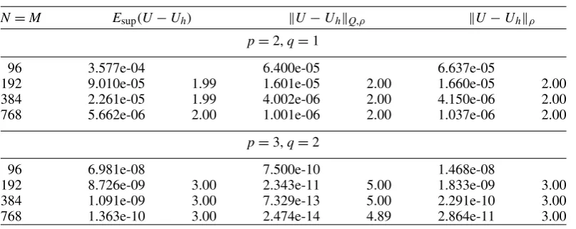
Remark3.18 The above analysis holds for all evolutionary problems and the above theorem gives error bounds for the semidiscrete solution of orderq+ 1, assuming enough regularity in time. In the case of less regularity Theorems3.8and3.12still hold. For a fully discrete method, a spatial discretization has to be defined too. This step, however, has to be done for each problem considered separately.
4. Full discretization for Example 1.3
Let us assume a regular, quasi uniform and shape-regular triangulationΩhof Ω into triangular open
cellsσ with maximal cell diameterh. Moreover, we assume that the interfaces betweenΩell,Ωparand
Ωhypare polygonal such that the triangulationΩhfits to these interfaces.
As the whole article is mainly concerned with the correct time discretization, in this section, we will employ the custom of the ‘generic constant’C 0 that may vary from line to line, which, however, depends onT,ρ,M1,M0,qandγand onk, the order of the assumed spatial regularity, only.
Then the fully discretized counterpartVτ
h toVis given by
Vhτ:=)(uh,vh)∈Vτ:uh|Im∈Pq(Im,V1(Ω)),vh|Im∈Pq(Im,V2(Ω)),m∈{1,. . .,M}
*
,
where the spatial spaces are
V1(Ω):=
v∈H01(Ω);∀σ : v|σ ∈Pk(σ ) , V2(Ω):= {w∈H(div,Ω);∀σ : w|σ ∈RTk−1(σ )}.
HerePk(σ )is the space of polynomials of degree up tokon the cellσ andRTk−1(σ) is the Raviart–
Thomas space, defined by
RTk−1(σ )=(Pk−1(σ ))n+xPk−1(σ ).
Note that
(Pk−1(σ ))n⊂RTk−1(σ )⊂(Pk(σ ))n,
div(RTk−1(σ ))⊂Pk−1(σ ) and
Furthermore, if the mesh consists of quadrilateral or hexahedral cells, in the above definitions and statements the polynomial space Pk(σ ) can be replaced by a mapped Qk space, including all polynomials of total degree k over a reference element and then mapped onto σ. If the mesh is a combination of both types of cells, a combination of spaces also works with a suitable mapping ensuring the continuities.
Remark 4.1 (Solvability of the fully discrete system) We can apply the general existence theory that was also used in Proposition3.2. More precisely, the positive definiteness still holds, since the triangulation fits to the interfaces and hence, the uniqueness of the system is warranted. However, since the problem is finite-dimensional, the uniqueness implies the existence of a solution of the fully discretized problem.
Let us come to the interpolation operatorI=(I1,I2). ForI1:C(Ω)→V1we use the Scott–Zhang
interpolant on each cellσ, see the study by (Scott & Zhang, 1990) for a precise definition, that is patched together continuously. Here local interpolation error estimates can be given usingL2norms also in 3d, which is not possible for standard Lagrange interpolation. ForI2:H(div,Ω)∩(Ls(Ω))n→V2 with s>2 we also use the standard interpolator, defined via moments, see the study by (Brezzi & Fortin, 1991). Note that in the following, in order to avoid a cluttered notation as much as possible, we will not explicitly keep track on the number of components of theL2(Ω) orHk(Ω) spaces under consideration,
as it will be obvious from the context.
Standard local interpolation error estimates yield for allv∈H10(Ω)∩Hr(Ω),
v−I1v0,Ω Chrvr,Ω, ∇(v−I1v)0,Ω Chr−1vr,Ω, (4.1) where 1 r k+1, see the study by (Scott & Zhang, 1990), and for all q ∈ Hs(Ω) such that
divq∈Hs(Ω)
q−I2q0,Ω Chsqs,Ω, div(q−I2q)0,Ω Chsdivqs,Ω, (4.2)
where 1sk, see the study by (Brezzi & Fortin, 1991).
LetUhτ ∈ Vhτ be the solution of the fully discretized system andPIU ∈ Vhτ be the interpolated solution of (1.1) for the operatorsM0,M1given in Example1.3andAgiven as in Example1.1. Then
we obtain analogously to the derivation of the errors of the semidiscretization
sup
t∈[0,T]
M0(PIU−Uhτ)(t),(PIU−Uhτ)(t)H+e2ρTPIU−Uτh2Q,ρ
Ce2ρT
∂tM0(U−PIU)2Q,ρ+ M1(U−PIU)2Q,ρ+ A(U−PIU)2Q,ρ
+T max
1mM
|M0(PIU−IU)(t+m−1)|2He−2ρtm−1
, (4.3)
where we remark that in contrast to Theorem3.8the termsM1(U−PIU)Q,2ρandA(U−PIU)2Q,ρ
convergence estimate in Theorem4.7. Beforehand, let us introduce
u2Q,ρ,k,D = M
m=1 Qm
|u|2k,D
e−2ρtm−1,
whereD⊆Ωis measurable.
Lemma4.2 It holds forU=(u,v)∈Hρ(R;Hk(Ω)×Hk(Ω))
U−PIUQ,ρ Chk
uQ,ρ,k,Ω + vQ,ρ,k,Ω
.
Moreover, ifU=(u,v)∈Hρ(R;D(A))such thatAU∈Hρ(R;Hk(Ω)×Hk(Ω)), then
A(U−PIU)Q,ρ Chk
uQ,ρ,k+1,Ω + divvQ,ρ,k,Ω
.
Proof. By the definition ofQm[·]ρwe have with (4.1) (r=k) and (4.2) (s=k)
U−PIU2Q,ρ = U−IU2Q,ρ= M
m=1 Qm
u−I1u20,Ω+ v−I2v20,Ω
e−2ρtm−1
C M
m=1 Qm
h2k|u(·)|2k,Ω +h2k|v(·)|2k,Ωe−2ρtm−1
=Ch2k u2Q,ρ,k,Ω + v2Q,ρ,k,Ω.
Very similarly we have for the second norm using (4.1) (r=k+ 1) and (4.2) (s=k)
A(U−PIU)2Q,ρ=
M
m=1 Qm
∇(u−I1u)20,Ω + div(v−I2v)20,Ω
e−2ρtm−1
Ch2k u2Q,ρ,k+1,Ω+ divv2Q,ρ,k,Ω.
Lemma4.3 It holds forU=(u,v)∈Hρ(R;Hk(Ω)×Hk(Ω))
M1(U−PIU)Q,ρ Chk
uQ,ρ,k,Ω + vQ,ρ,k,Ω
.
Lemma4.4 ForU=(u,v)∈Hρ1(R;Hk(Ω)×Hk(Ω))∩Hρq+2(R;L2(Ω)×L2(Ω))we have sup
t∈[0,T]
M0(U−PIU)(t),(U−PIU)(t)H
C
h2k sup
t∈[0,T]
|u(t)|k,Ω + |v(t)|k,Ω
2
+τ2(q+1) sup
t∈[0,T]|
∂tq+1IU(t)|2H
.
Proof. The operatorM0is selfadjoint and non-negative. Thus it follows that M0(U−PIU)(t),(U−PIU)(t)H= |
(
M0(U−PIU)(t)|2H
2 |(M0(U−IU)(t)|2H+ | (
M0(IU−PIU)(t)|2H
for eacht∈[0,T]. The second term can be estimated by |(M0(IU−PIU)(t)|2H Cτ2(q+1) sup
t∈[0,T]|
∂tq+1IU(t)|2H
according to Lemma3.15, while the first term can be estimated by
|(M0(U−IU)(t)|2L2(Ω)Ch2k |u(t)|2k,Ω+ |v(t)|2k,Ω
,
due to the boundedness of√M0. Hence, the assertion follows.
Lemma4.5 ForU=(u,v)∈Hρ1(R;Hk(Ω)×Hk(Ω))∩Hq+3
ρ (R;L2(Ω)×L2(Ω)), we get
∂tM0(U−PIU)2Q,ρ C
h2k∂tuQ,ρ,k,Ω + ∂tvQ,ρ,k,Ω2+τ2(q+1) sup
t∈[0,T]|
∂tq+2IU(t)|2H
.
Proof. We have that
∂tM0(U−PIU)Q,ρ ∂tM0(U−IU)Q,ρ+ ∂t(M0IU−PM0IU)Q,ρ
M0(∂tU−I∂tU)Q,ρ+Cτq+1 sup
t∈[0,T]|
∂tq+2IU(t)|H,
by Lemma3.13. For the first term we have by Lemma4.2
M0(∂tU−I∂tU)2Q,ρ Ch
2k
∂tu2Q,ρ,k,Ω + ∂tv2Q,ρ,k,Ω
.
Lemma4.6 It holds forU=(u,v)∈Hρq+2(R;L2(Ω)×L2(Ω)) max
1mM)M0(PIU−IU)
t+m−1L2(Ω)e−ρtm−1 *
Cτq+1 sup
t∈[0,T]|