City, University of London Institutional Repository
Citation
: Rendon, J. & de Menezes, L. M. (2017). Structural combination of neural
network models. 2016 IEEE 16th International Conference on Data Mining Workshops
(ICDMW), pp. 406-413. doi: 10.1109/ICDMW.2016.0064
This is the accepted version of the paper.
This version of the publication may differ from the final published
version.
Permanent repository link:
http://openaccess.city.ac.uk/17598/
Link to published version
: http://dx.doi.org/10.1109/ICDMW.2016.0064
Copyright and reuse:
City Research Online aims to make research
outputs of City, University of London available to a wider audience.
Copyright and Moral Rights remain with the author(s) and/or copyright
holders. URLs from City Research Online may be freely distributed and
linked to.
City Research Online:
http://openaccess.city.ac.uk/
[email protected]
Structural combination of neural network models
Juan Rendon
Cass Business School City, University of LondonLondon, UK
Email: [email protected]
Lilian M. de Menezes
Cass Business School City University of LondonLondon, UK
Email: [email protected]
Abstract—Forecasts combinations normally use point forecasts that were obtained from different models or sources ([1], [2], [3]). This paper explores the incorporation of internal structure parameters of feed-forward neural network (NN) models as an approach to combine their forecasts via ensembles. First, the gen-erated NN models that could be part of the ensembles are subject to a clustering algorithm that uses the structure parameters and, from each of the clusters obtained, a small set of models is selected and their forecasts are combined in a two-stage procedure. Secondly, in an alternative and simpler implementation, a subset of the generated NN models is selected by using several reference points in the model structure parameter space. The choice of the reference points is optimised through a genetic algorithm and the models selected are averaged. Hourly electricity demand time series is used to assess multi-step ahead forecasting performance for up to a 12 hours horizon. Results are compared against several statistical benchmarks, the average of the individual forecasts and the best models in the ensembles. Results show that the cluster-based (CB) structural combinations do better than the genetic algorithm (GA) structural combinations in outperforming the average forecast, which is the traditional point forecast from an ensemble.
I. INTRODUCTION
The term ensemble originated in climate modelling, where scientists distinguish different types of uncertainty, as [4] described. Structural uncertainty refers to uncertainty about the form that the modelling equations should take;parametric uncertainty is about the values that should be assigned to parameters within a set of modelling equations andinitial con-dition uncertainty, which refers to the difficulty in measuring all the required variables needed in models.
Ensembles were adopted in NNs by [5], and came to mean the use of several models, constructed with differences in one or more of their design parameters. They used ensembles of NNs for classification. In this seminal research only synthetic data were used, and superiority of the ensemble was reported in comparison to individual models. Since this research, NN ensembles have evolved from the use of simple sets of models to the collective evolution of them through sophisticated computational intelligence techniques.
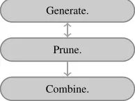
Ensembles involve three main tasks, as depicted in Figure 1: generation, pruning and combination. Generation involves the creation of different models. Pruning comprises a selection of them, and is optional ([6]). The final stage performs the combination of forecasts. Other factors to be considered are: the type of model to ensemble, how the individual models
are produced, the level of automation of the process and the way combinations are made. Therefore the construction of ensembles is far more complex than the construction of a single model.
Generate.
Prune.
[image:2.612.389.486.256.329.2]Combine.
Fig. 1. General steps in ensemble generation.
There are sequential approaches where the generation of models is followed by a pruning stage and finished with a combination stage (see for example [7]). But in other ap-proaches this sequence is not entirely observed: the evolution (or generation) of the individual models can be done in parallel, so that the information from the training stage can be shared, and used to modify the collective estimation of parameters ([8] ,[9]).
The type of model used and the generation process are in-terrelated. The most common types of models in the literature are feed-forward NNs (e.g. [5] , [10]), although Radial Basis Functions ([11], [12]), Elman recurrent network and Hopfield ([12]), Deep belief network ([13]) and Abductive networks ([14]) can also be found.
Once the type of model is chosen, a question arises about how to specify the individual models. In the case of feed-forward NN, the creation of a single model for forecast-ing requires several parameters, which can be determined by trial and error, heuristic rules or systematic approaches. For example, [15] conducted model selection with strategies based on sequential statistical tests, information criteria and cross validation. [16] and [17] use design of experiments to identify an appropriate network configuration. [18] emphasised input selection, as part of model specification, and proposed a methodology for seasonal components. Nevertheless, no universal guideline exists on how to select the appropriate model ([19]).
samples ([7], [21]). The randomisation of the feature space ([9]) could count both as a strategy for model variation and as a strategy for model specification.
In the final block in Figure 1, models are combined to produce the output of the ensemble. The methods that have been proposed in the literature (focusing on forecasting rather than on classification) include: a gating network ([22]), a simple or weighted average ([8], [12], [23], [24]), a nonlinear average through another NN ([23]), a feed-forward NN ([25], [26]), a Radial Basis Function ([11]), the median of forecasts ([10], [20]) and the mode ([19]). It can be seen that the complexity and effectiveness of the ensembling approaches are only partially related to the combining procedure at the end of the process, as there are other steps involved.
In the energy forecasting area the use of NN ensembles is common. [27] and [28] forecasted hourly electricity demand and gas consumption, respectively, by using feed-forward NNs. Forecasts were combined through the average, recursive least squares, fuzzy logic, feed-forward NN, functional link NN, a partition of the temperature space (an external vari-able), a linear programming algorithm and a mixture of local experts. The best performance was obtained with a NN as a combination mechanism.
[29] forecasted hourly and peak load (with data from two US utilities) for the next 24 and 120 hours with a small ensemble of NNs. K-nearest neighbour was used to select training sets. NNs were trained in parallel with an itera-tive approach, feeding back averaged forecasts as inputs for subsequent forecast horizons. Results were competitive when compared with usual forecast error measures in similar utilities and previous publications .
[30] used NNs to produce load forecasts from 1 to 10 days ahead based on ensembles of weather forecasts. Comparisons were made with uni-variate benchmarks and point forecasts from individual models. For ten lead times, the mean of the load scenarios built with weather variables was a more accurate forecast than that produced by the non-ensemble based procedure. This research combines the use of ensemble weather forecasts with an ensemble of rather low complexity NNs leading to a improvements in forecast accuracy. Variety in the data is not needed as different scenarios are used as inputs.
Further research involving combination of forecasts pro-duced with different types of NNs include [10], [13], [14], [26], [31], [32] and [33]. In general, there is limited research on forecast combination approaches that consider the internal characteristics of the models involved. [21] suggested this direction, by considering clustering of structural parameters to summarise models based on such clusters. This line of thought can be further explored, in terms of the clustering techniques and the kind of time series to be considered.
This paper proposes one form of structural combination, implemented in two ways: one with a recursive partitioning of the weights space of NNs to then select models to combine, and another with a Genetic Algorithm which searches for reference points in such parameter space to select models to
combine. The next sections describe the method and illustrate their use in forecasting electricity demand from Rio de Janeiro 12 hours ahead.
II. METHODOLOGY
The most common types of NN models in the literature of ensemble development are feed-forward NNs (see for example [5] and [10]). Such NNs are common in forecasting ([34], [18]) and, specifically, in the electricity sector (i.e. [27], [29], [14]). Multi-layer perceptrons are the most frequently applied ([34]) and, therefore, are adopted here.
Figure 2 describes the modelling process. A base NN struc-ture, which has been selected through a preliminary process (such as a sensitivity analysis or a heuristic approach, e.g. [17]), is used to fit the time series with different models. Parameter diversity can be introduced through various mech-anisms, one of which is the randomisation of input-output patterns for the neural networks, which is adopted here and is described in the next subsection. Once the ensemble is generated, the models are subject to a combination procedure involving the structure, as described below, and, finally, fore-casts are produced and their uncertainty assessed.
The modelling process depends on specific design decisions. The combination algorithm, the forecast stage, the uncertainty assessment and the multi-step ahead forecast approach used to fit the individual models can influence each other. In an iterative approach, where a network produces forecasts for all horizons, the modelling process leads to a single ensemble that forecasts different horizons.
A. Randomisation of input-output patterns
The pre-processing stage uses randomisation of input-output data patterns during the training period. This mechanism facilitates the creation of diverse NN models (with different parameter sets), thus facilitating the identification of different clusters of models in the parameter space.
B. Structural Combination based on Clustering
When the structural combination stage in Figure 2 is implemented through clustering, the combination becomes a mechanism that looks into the structure of models and finds groups in the space defined by such structure. An algorithm based on fuzzy C-means was chosen, which incorporates concepts from fuzzy systems.
Fuzzy C-Means is an algorithm that partitions a collection of vectors intocfuzzy groups and finds a cluster centre in each group such that a cost function of dissimilarity is minimised (see [35]). The choice of a fuzzy C-means oriented approach is due to its use of a degree of membership of elements to clusters (between 0 and 1), instead of a binary membership (0 or 1, equivalent tonon-memberandmember in K-means). Therefore, a NN model can belong to several clusters with different degrees of belongingness that are defined by grades between 0 and 1 ([35, p. 426]).
Data.
Randomised input-output data patterns.
Randomised input-output data patterns.
.. .
Randomised input-output data patterns.
N N1
N N2
.. .
N Nk
Structural
combination Forecast.
[image:4.612.69.491.50.181.2]Assessment of uncertainty in forecast.
Fig. 2. Modelling process.
based on [36], which uses a recursive partitioning of the model space that helps in producing a deterministic partition. The next sub-section describes the model in detail.
C. The forecasting model
The clustering-based algorithm (CB) uses structure informa-tion of models and produces forecasts based on the data and this information. It creates partitions in the parameter space of the NNs and centres of such regions are used as cluster centres. When the individual NN models are used to issue forecasts in an iterative manner, the clustering procedure takes into account the in-sample one-step-ahead forecasts produced by NNs in order to calculate the loss function, which is to be minimised. The forecast for each horizonhis calculated based on the forecasts made by the clustered NNs for the respective horizon, as follows:
ˆ
yh= n
X
i=1
φiyˆCi,h (1)
WhereyˆCi,h is the forecast from clusteri for horizonh:
ˆ
yCi,h=α0+α1Mi1(h) +α2Mi2(h) +. . .+αLMiL(h) (2)
Mi1(h), Mi2(h), . . . are forecasts for step ahead h from
models selected within cluster i.
The coefficients φk are calculated as an average of the
normalised weights of vectors (models in vectorial form):
φk=
PNk
i=1wk
Nk
(3)
whereNk is the number of models in clusterk.
wi(v) =
ui(v)
Pn
j=1uj(v)
(4)
ui(v) =e
− D2i(v) Pn
j=1D2j(v) (5)
ui(v) is the membership of v to cluster i (v is a model
represented in the form of a vector). The squared distance between v and the i-th centre is divided by the sum of squared distances from v to all centres. Subsequently, an exponential transformation is taken so that the membership
of a model to a cluster decreases as long as its distance from the centre increases. Consequently, there is always a degree of membership, however small, of every vector to every cluster.
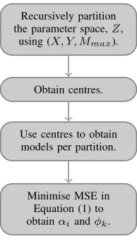
Recursively partition the parameter space,Z,
using (X, Y, Mmax).
Obtain centres.
Use centres to obtain models per partition.
[image:4.612.389.486.258.429.2]Minimise MSE in Equation (1) to obtainαiandφk.
Fig. 3. Clustering Scheme.
The partitioning routine, in Figure 3, which is used to build the clusters, recursively splits the parameter space of models in two steps. A forward step, which grows partitions in the form of a tree and a backward step, which prunes those regions that do not improve fit function (MSE).
X is the set of input variables, including lagged values of the dependent variable,Y is the one step ahead forecast for the independent variable. The recursive partitioning uses internally a matrix Z, where every row represents a model (a NN) in the parameter space, which has already been trained with the
X, Y data set. Mmax is the maximum number of clusters
allowed.
In the first step of Figure 3, a procedure
regressByCluster(X, Y, B) is internally used, which performs an OLS regression of Y on X in a per-cluster manner, with B containing the definitions of the regions or clusters. This gives initial estimates of αandφthat are then updated in the last stage of Figure 3.
The regions,B, are defined in the form of base functions:
Bm(Z) = Km Y
k=1
H skm· zv(k,m)−tkm
H(η) =
1if η≥0
0 otherwise (7)
For a vectorz, the functionBm(z)establishes ifz belongs
to the m-th region. If so, the function takes the value 1. If
z does not belong to the region, the function would have the value 0. Km is the number of partitions in the space that
define the region. skm is a constant that takes the values 1 or
-1, signalling if the partition is to the right or to the left of the value tkm. The variable zv is the dimension, in the space
of parameters, in which a partition is made.
Both the individual NNs and the CB algorithms were imple-mented in MatlabR 2010 using its neural networks toolbox.
D. Structural combination based on genetic algorithms
The cluster-based implementation described in the previous subsection creates clusters that serve to extract and combine models. A simplified implementation was conducted by using genetic algorithms. Again, X is the set of input variables, including lagged values of the dependent variable, Y is the one step ahead forecast for the independent variable andZ is a matrix where every row represents a model (a neural network) in the parameter space, which has already been trained with the X,Y data set.
A series of reference points in the parameter space is generated. From each point, Pi, a number of NN models is selected, having the smallest euclidean distance to it. The forecast produced by this combination (yAvg) is calculated as
the average forecast of all models selected from all reference points (5 models are selected from each point, as specified in Table I). The routine optimises through a genetic algorithm the set of reference points such that the MSE of the yAvg
in-sample one-step-ahead point forecasts is minimised. A GA combination can be viewed as a structurally informed average: it selects models based on closeness around different points in the parameter space and then performs an average. The algorithm is run over the same NN pool used to perform the structural combination proposed in previous subsections. It was implemented in MatlabR 2010 usinggaroutine, setting a maximum number of generations to 3000.
III. STUDY WITH AN ELECTRICITY DEMAND TIME-SERIES
A time series of electricity demand was used to asses the performance of CB and GA structural combination ap-proaches. The series contains hourly observations in Rio de Janeiro covering the period from Sunday 5 May 1996 to Saturday 30 November 1996 (Figure 4). It has been used by [37] to evaluate the performance of various uni-variate models, including a NN, which was implemented according to [38].
The direct approach of fitting different NNs for different forecast horizons led to a performance markedly different from results obtained by [37]. In their study, the authors fitted a NN with input lags 1, 2, 24, 25, 48, 72, 96, 120, 144, 168, 192, 216, 240, 264, 312, 336 and forecasted the differences in an iterative manner. Further experiments with this setting provided better results than the direct approach and therefore it was adopted for the present study.
A preliminary analysis suggested that an NN architecture with 16 inputs (corresponding to all lags considered) and 2 neurons would be the best choice. Such architecture is used here with the CB and GA procedures described above to test the structural combination of forecasts. Due to the existence of extreme values in the out-of-sample performance of NNs, the ensemble to perform the combination was built with the over-produce and choose approach ([6]): 150 NNs where generated and 50 selected. The forecast performance for h = 12 was assessed with a rolling window in the in-sample period and the best models were used to conduct the structural combination. The configurations of the individual NNs and combination algorithms is summarised in Table I.
Results are compared with those obtained by [37] with a Holt-Winters-Taylor (HWT) exponential smoothing method and a NN. Comparisons are made by using MSE and MAPE error metrics.
TABLE I STUDY CONFIGURATION.
Individual NN configuration. Factor Values
Num. inputs 1, . . . ,16, being 16 the number of lags. Num. hidden layers 1
Num. hidden units 2
Activation function for hidden nodes
Tangent Sigmoid
Activation function for the output node
Linear
Initial values for the weights
Values in the range [-2 [-2] established by the Nguyen-Widrow algo-rithm
Training algorithm Backpropagation with Levenberg-Marquardt optimisation and Bayesian regularization Data normalisation Yes
Init. Combination coef-ficient (µ)
0.001
Sample size 5040
Data config. for train-ing, testing and valida-tion
N tr = 3024, N va = 336N te= 1680
Extreme values treated No. Forecast approach Iterative
Combination configuration.
Num. of models 50
Num. Max. clusters 2, 4, 8 Models per cluster 5
Final combination Linear Randomised
input-output patterns
Yes
Structural content All synaptic weights in each NN.
Fig. 4. Hourly electricity demand in Rio de Janeiro for Sunday, 5 May 1996 to Saturday, 30 November 1996. Original Series.
percentage differences are calculated only for models derived from the NNs produced in the study. Table II provides sample coefficients for CB models. The assessment of uncertainty in forecasts, by using forecast intervals, is provided in Figure 7 (only CB models are considered).
TABLE II
COEFFICIENTS FOR STRUCTURAL COMBINATION OFNNFORRIO DEJANEIRO ELECTRICITY DEMAND SERIES.
CB2
α1 24.9383 0.38 0.4028 0.0896 -0.0942 0.2126
Φ 1
CB4
α1 25.3822 0.7965 -1.7627 1.1277 0.2929 -0.4866
α2 26.3815 -1.0451 3.2846 0.5185 1.8219 1.4281
α3 28.9069 0.5246 -2.3253 0.5201 0.8754 0.2391
Φ 0.3984 0.1786 0.4233 CB8
α1 24.9104 1.4617 -5.6481 2.2431 0.3346 0.1906
α2 26.1478 1.7667 6.8272 0.5522 3.0498 1.7813
α3 27.6467 -2.071 1.087 0.9352 0.0621 0.3737
α4 21.5636 -2.3524 0.62 -0.3881 1.4783 -1.4435
α5 29.9801 -6.0529 1.2764 2.8328 0.9112 1.7857
Φ 0.2199 0.1086 0.2297 0.2243 0.2169
αi are the coefficients applied to point-forecasts from models in clusteriand Φare the weights applied to the outputs from clusters. Theαin the first column (αi,0) is the intercept of the linear combination. Theαi,j, forj >0, in the remaining columns, are applied to point forecasts.
IV. DISCUSSION
It is noticeable that not only the best performing NNs for the electricity demand series are simple in terms neurons, but also the best performing CB models are the simplest. For example, CB2, with a maximum of 2 clusters, was able to consistently outperform the average forecast from the NNs. The need for structural simplicity in the case of the electricity demand series is manifested both at single model and at ensemble level.
This time series required a sensible selection of inputs in the early stages of the study, so as to capture the regularities in the series, in accord with [18]. However, this also implies that the the statistical benchmarks are very well suited to the data, and thus the NN models and ensembles had difficulty in outperforming the well specified models. It thus appears that
faced with regular data, it pays off to invest time and effort in the selection of inputs and use a well-specified model that address these regularities to forecast the series.
Larger structural representations of models can be used. However, their complexity could create challenging features to perform structural combinations. A proper balance between dimension reduction and the use of a sufficiently rich structural representation would be needed to achieve practical computing times.
Replacing the randomisation of the training set by a boot-strap strategy to create the individuals models that participate in the clustering algorithm, would move the approach in the di-rection of bagging. The GA combination can also benefit from such modification and these are potential research avenues for future research.
V. CONCLUSION
This paper presents a novel forecasting combination ap-proach that involves the creation of ensembles of NNs and the combination of a subset of them based on parameters from their structure. The first implementation of the proposed combination approach is based on clustering algorithms, which groups together models that share a measure of similarity (in this case, a measure of distance in the parameter space of models). The second implementation uses genetic algorithms to select models by using reference points (analogous to cluster centres) in the parameter space and can be seen as a structurally informed average of forecasts. Different levels in the number of clusters were used to assess the combinations. For the double-seasonal time series considered here the CB tend to do better in relation to the simple average combination. Furthermore, there is no marked superiority of structural combinations over individual models. In spite of this, CB shows better performance than GA with respect to the best models.
[image:6.612.51.298.342.480.2]Fig. 5. Out-of-sample MAPE for Rio de Janeiro electricity demand series.
Ranking of models (MAPE). % difference wrt. Average (MAPE).
Ranking of models (MSE). % difference wrt. Average (MSE).
Fig. 6. Comparison by forecast horizon. Best model is in rank 1. % differences with respect to the average are negative when there is improvement over the average benchmark. CB2 stands for a cluster-based combination with a maximum of 2 clusters. GA2 stands for a genetic-algorithm based combination with 2 reference points. Bst. ismape denotes the NN in the study with the lowest in-sample MAPE. Bst. ismse denotes the NN with the lowest in-sample MSE. HWT Taylor and NN Taylor denote results from [37].
attractive in the case of double-seasonal time series data. Nonetheless, it is noteworthy that HWT has an in-built error correction mechanism, which is not present in the NNs. Given changes in the data pattern within the out-of-sample period, as observed in this time series, structural combinations of recursive neural networks become an attractive avenue for research.
Based on these findings, future research could investigate the behaviour of a structural combination approach when models of different nature are combined. If, for example, instead of using single single unit models (statistical or com-putational intelligence model), bundles of the form Bi =<
ARIM A, N N > are formed, the structural combination of such bundles could potentially improve performance, when dealing with complex forecasting problems.
Other forms of structural representation can be envisaged, while taking care of keeping a reasonable computing cost. Changes in the generation of individual models could lead to approaches closer to bagging, thus facilitating the exploration of research avenues that could improve forecasting perfor-mance.
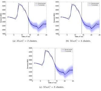
[image:7.612.119.504.215.505.2](a) M axC= 2clusters. (b)M axC= 4clusters.
[image:8.612.135.469.54.356.2](c)M axC= 8clusters.
Fig. 7. Forecast intervals for Rio electricity demand time series.
The graphs cover the period for t−12 ≤ t ≤ t+H where t is the last observation of the in-sample period and H = 12 is the number of forecast horizons. The shades, from lighter to darker, correspond to αlevels 0.95, 0.90, 0.85, 0.80, 0.75 and 0.60.
series, suggests that an extension of the present research could investigate how the chosen multi-step-ahead forecast approach affects the performance of structural combination.
Overall, the exploration of structural combination of fore-casts, and its implementation in two forms, open the possibility to investigate new forms of ensembles, specially when rela-tionships between components in the individual models can be clearly distinguished.
REFERENCES
[1] P. Newbold and C. W. Granger, “Experience with forecasting univariate time series and the combination of forecasts,” Journal of the Royal Statistical Society. Series A (General), pp. 131–165, 1974.
[2] R. T. Clemen, “Combining forecasts: A review and annotated bibliography,” International Journal of Forecasting, vol. 5, no. 4, pp. 559 – 583, 1989. [Online]. Available: http://www.sciencedirect.com/science/article/pii/0169207089900125 [3] A. Timmermann, “Chapter 4 forecast combinations,” ser. Handbook
of Economic Forecasting, C. G. G. Elliott and A. Timmermann, Eds. Elsevier, 2006, vol. 1, pp. 135 – 196. [Online]. Available: http://www.sciencedirect.com/science/article/pii/S1574070605010049 [4] W. S. Parker, “Predicting weather and climate: Uncertainty, ensembles
and probability,” Studies In History and Philosophy of Science Part B: Studies In History and Philosophy of Modern Physics, vol. 41, no. 3, pp. 263–272, Sep. 2010. [Online]. Available: http://linkinghub.elsevier.com/retrieve/pii/S1355219810000468 [5] L. K. Hansen and P. Salamon, “Neural network ensembles,” IEEE
Transactions on Pattern Analysis and Machine Intelligence, vol. 12, no. 10, pp. 993–1001, 1990.
[6] J. Mendes-Moreira, C. Soares, A. M. Jorge, and J. F. D. Sousa, “En-semble approaches for regression: A survey,”ACM Computing Surveys (CSUR), vol. 45, no. 1, p. 10, 2012.
[7] Z.-H. Zhou, J. Wu, and W. Tang, “Ensembling neural networks: Many could be better than all,” Artificial Intelligence, vol. 137, no. 1-2, pp. 239–263, May 2002. [Online]. Available: http://linkinghub.elsevier.com/retrieve/pii/S000437020200190X [8] Y. Liu, X. Yao, and T. Higuchi, “Evolutionary ensembles with
negative correlation learning,” IEEE Transactions on Evolutionary Computation, vol. 4, no. 4, pp. 380–387, 2000. [Online]. Available: http://ieeexplore.ieee.org/lpdocs/epic03/wrapper.htm?arnumber=887237 [9] H. Chen and X. Yao, “Evolutionary random neural
ensembles based on negative correlation learning.” Ieee, Sep. 2007, pp. 1468–1474. [Online]. Available: http://ieeexplore.ieee.org/lpdocs/epic03/wrapper.htm?arnumber=4424645 [10] S. Fan, L. Chen, and W.-j. Lee, “Short-Term Load Forecasting Using Comprehensive Combination Based on Multimeteorological Informa-tion,”IEEE Transactions on Industry Applications, vol. 45, no. 4, pp. 1460–1466, 2009.
[11] L. Yu, K. K. Lai, and S. Wang, “Multistage RBF neural network ensemble learning for exchange rates forecasting,” Neurocomputing, vol. 71, no. 16-18, pp. 3295–3302, Oct. 2008. [Online]. Available: http://linkinghub.elsevier.com/retrieve/pii/S0925231208003020 [12] I. Maqsood, M. Khan, and A. Abraham, “An ensemble of neural
networks for weather forecasting,”Neural Computing and Applications, vol. 13, no. 2, pp. 112–122, May 2004. [Online]. Available: http://link.springer.com/10.1007/s00521-004-0413-4
[13] X. Qiu, L. Zhang, Y. Ren, and P. N. Suganthan, “Ensemble Deep Learning for Regression and Time Series Forecasting,” 2014. [14] R. E. Abdel-Aal, “Improving electric load forecasts using network
committees,”Electric Power Systems Research, vol. 74, no. 1, pp. 83–94, 2005.
networks : the official journal of the International Neural Network Society, vol. 12, no. 2, pp. 309–323, Mar. 1999. [Online]. Available: http://www.ncbi.nlm.nih.gov/pubmed/12662706
[16] G. P. Zhang, B. E. Patuwo, and M. Y. Hu, “A simulation study of arti-ficial neural networks for nonlinear time-series forecasting,”Computers & Operations Research, vol. 28, pp. 381–396, 2001.
[17] P. Balestrassi, E. Popova, a.P. Paiva, and J. Marangon Lima, “Design of experiments on neural network’s training for nonlinear time series forecasting,” Neurocomputing, vol. 72, no. 4-6, pp. 1160–1178, Jan. 2009. [Online]. Available: http://linkinghub.elsevier.com/retrieve/pii/S0925231208001513 [18] S. F. Crone and N. Kourentzes, “Feature selection for
time series prediction – A combined filter and wrapper approach for neural networks,” Neurocomputing, vol. 73, no. 10-12, pp. 1923–1936, Jun. 2010. [Online]. Available: http://linkinghub.elsevier.com/retrieve/pii/S0925231210000974 [19] N. Kourentzes, D. K. Barrow, and S. F. Crone, “Neural network
ensemble operators for time series forecasting,”Expert Systems with Applications, vol. 41, no. 9, pp. 4235–4244, 2014. [Online]. Available: http://www.sciencedirect.com/science/article/pii/S0957417413009834 [20] P. J. Adeodato, A. L. Arnaud, G. C. Vasconcelos, R. C. Cunha,
and D. S. Monteiro, “MLP ensembles improve long term prediction accuracy over single networks,”International Journal of Forecasting, vol. 27, no. 3, pp. 661–671, Jul. 2011. [Online]. Available: http://linkinghub.elsevier.com/retrieve/pii/S0169207009000995 [21] B. Bakker and T. Heskes, “Clustering ensembles of neural network
models.” Neural networks : the official journal of the International Neural Network Society, vol. 16, no. 2, pp. 261–269, Mar. 2003. [Online]. Available: http://www.ncbi.nlm.nih.gov/pubmed/12628611 [22] R. Jacobs and M. I. Jordan, “A competitive modular connectionist
architecture,” in Advances in Neural Information Processing Systems 3, L. R.P., J. Moody, and D. Touretzky, Eds. Morgan-Kaufmann, 1991, vol. 2, pp. 767–773.
[23] V. M. Krasnopolsky, “Reducing uncertainties in neural network Jacobians and improving accuracy of neural network emulations with NN ensemble approaches.” Neural networks : the official journal of the International Neural Network Society, vol. 20, no. 4, pp. 454–61, May 2007. [Online]. Available: http://www.ncbi.nlm.nih.gov/pubmed/17521879
[24] M. M. Islam, X. Yao, and K. Murase, “A constructive algorithm for training cooperative neural network ensembles.”IEEE transactions on neural networks / a publication of the IEEE Neural Networks Council, vol. 14, no. 4, pp. 820–34, Jan. 2003. [Online]. Available: http://www.ncbi.nlm.nih.gov/pubmed/18238062
[25] L. Yu, S. Wang, and K. Lai, “A novel nonlinear ensemble forecasting model incorporating GLAR and ANN for foreign exchange rates,” Computers & Operations Research, vol. 32, no. 10, pp. 2523–2541, Oct. 2005. [Online]. Available: http://linkinghub.elsevier.com/retrieve/pii/S030505480400156X [26] L. Yu, S. Wang, and K. K. Lai, “Forecasting crude oil price with an
EMD-based neural network ensemble learning paradigm,”Energy Eco-nomics, vol. 30, no. 5, pp. 2623–2635, Sep. 2008. [Online]. Available: http://linkinghub.elsevier.com/retrieve/pii/S0140988308000765 [27] A. Khotanzad, R. Afkhami-Rohani, and D. Maratukulam, “ANNSTLF
- Artificial Neural Network Short-Term Load Forecaster - Generation Three,”IEEE Transactions on Power Systems, vol. 13, no. 4, pp. 1413– 1422, 1998.
[28] A. Khotanzad, H. Elragal, and T. L. Lu, “Combination of artificial neural-network forecasters for prediction of natural gas consumption.” IEEE transactions on neural networks, vol. 11, no. 2, pp. 464–73, Jan. 2000. [Online]. Available: http://www.ncbi.nlm.nih.gov/pubmed/18249775
[29] I. Drezga, “Short-term load forecasting with local ANN predictors,”
IEEE Transactions on Power Systems, vol. 14, no. 3, pp. 844–850, 1999. [30] J. W. Taylor and R. Buizza, “Neural network load forecasting with weather ensemble predictions,”IEEE Transactions on Power Systems, vol. 17, no. 3, pp. 626–632, 2002.
[31] H. Daneshi and A. Daneshi, “Real Time Load Forecast in Power System,” inElectric Utility Deregulation and Restructuring and Power Technologies, 2008. DRPT 2008. Third International Conference on, no. April, 2008, pp. 689–695.
[32] D. Fay and J. V. Ringwood, “On the Influence of Weather Forecast Errors in Short-Term Load Forecasting Models,”IEEE Transactions on Power Systems, vol. 25, no. 3, pp. 1751–1758, 2010.
[33] S. Hassan, A. Khosravi, and J. Jaafar, “Examining performance of aggregation algorithms for neural network-based electricity demand forecasting,” International Journal of Electrical Power & Energy Systems, vol. 64, pp. 1098–1105, 2015. [Online]. Available: http://linkinghub.elsevier.com/retrieve/pii/S0142061514005511 [34] S. F. Crone and R. Dhawan, “Forecasting Seasonal Time Series
with Neural Networks: A Sensitivity Analysis of Architecture Parameters.” Ieee, Aug. 2007, pp. 2099–2104. [Online]. Available: http://ieeexplore.ieee.org/lpdocs/epic03/wrapper.htm?arnumber=4371282 [35] J. Jang, C. Sun, and E. Mizutani, Neuro-fuzzy and soft computing: a computational approach to learning and machine intelligence. Prentice Hall, 1997. [Online]. Available: http://books.google.co.uk/books?id=vN5QAAAAMAAJ
[36] J. H. Friedman, “Multivariate adaptive regression splines,”The Annals of Statistics, vol. 19, no. 1, pp. 1–67, 1991. [Online]. Available: http://www.jstor.org/stable/2241837
[37] J. W. Taylor, L. M. de Menezes, and P. E. McSharry, “A comparison of univariate methods for forecasting electricity demand up to a day ahead,” International Journal of Forecasting, vol. 22, no. 1, pp. 1–16, Jan. 2006. [Online]. Available: http://linkinghub.elsevier.com/retrieve/pii/S0169207005000907 [38] G. A. Darbellay and M. Slama, “Forecasting the short-term demand for