Thomas A McMaster*, Xiu T Yan**
*Department of Design, Manufacture and Engineering Management (DMEM), University of Strathclyde, 75 Montrose Street, Glasgow, United Kingdom, G1 1XJ; (Tel: 0141 574 5197, e-mail: [email protected]).
**Department of Design, Manufacture and Engineering Management (DMEM), University of Strathclyde, 75 Montrose Street, Glasgow, United Kingdom, G1 1XJ; (e-mail: [email protected])
Abstract: The additive manufacture process is thermally-complex – many different material mechanisms are occurring due to the heating/cooling cycle that parts are put through when the material is deposited. This complexity is compounded when parts are made from a combination of materials, as in functionally graded material (FGM) parts. To better understand this complexity, a Python™ code has been developed to plot heat flow through the part as material is being deposited. The outputs of such code will highlight the influence of the deposition tool path and indicate to the engineer what areas of a part may require redesigning. A robotic arm gripper is used as a test bed throughout the development of the code.
Keywords: Heat Flow, Additive Manufacture, Functionally Graded Materials, Robotic Arm Gripper, Python™
1. INTRODUCTION
Heat flow is an important consideration when additively manufacturing a part, as residual heat can cause side effects, such as warping [1]. The ability to simulate this heat flow is thus important, especially when creating FGM parts, due to their unpredictable heat flow characteristics. Heat flow through single-material parts is possible with a range of off-the-shelf products [2, 3], however, it is not commonplace when the part has a varying material composition. The development of a code capable of this would therefore be beneficial.
This paper aims to develop this code using Python™ scripts written for Abaqus™ finite element software. The code will allow engineers to study the impact of thermal effects from an additive manufacture process on parts being designed. The engineer will be able to establish if temperatures during manufacture are too high at any points in the designed part and alter the design and/or materials to reduce temperatures, if need be. When used in conjunction with the methodology from McMaster et al [4], the heat flow code presented in this paper gives a holistic approach to redesigning structural mechatronic components.
This paper will be structured as follows: section 2 will be contain a brief description of FGMs, section 3 will detail the development and creation of the heat flow code itself, section 4 will introduce the test part used for validation, section 5 will show the resulting outputs of the heat flow code on the test part, section 6 will discuss the implementation of the code and its effectiveness, section 7 will conclude and section 8 will give suggestions for future work, which include building and testing of physical parts to garner information that can be used to further develop the simulation code in this
paper and inclusion into the code of mechanics to simulate the bond layer between different layers in the functionally graded materials.
2. FUNCTIONALLY GRADED MATERIALS
FGMs are a category of advanced materials that vary their properties over distance. FGMs are classified by their gradation technique - either porosity or composition, or a combination of the above. These are seen in Fig. 1. They can either be made on as bulk parts or as thin parts (for example, surface coatings). The structure can either be discrete or continuous, as visualised in Fig. 2.
Using this process allows different mechanical properties to be realised at specific areas of a part, while ensuring that stress concentrations do not arise due to distinct material bonds. The outcome is a part with task-specific properties at different points in the part’s geometry
The code in this paper is designed for bulk, composition-based discrete parts, though, as the processes are similar for the other FGM classifications, the ideas in this work can be adapted to suit the other classifications.
[image:1.595.442.548.645.728.2]Graded by porosity [5] Graded by microstructure [6]
Continuous structure Discrete structure
Fig. 2: FGM Structure options
3. HEAT FLOW CODE
The heat flow code was written in Python in order for it to be read by Abaqus. This choice of software was made to ensure two conditions: 1) for integration purposes with the other steps in the researcher’s methodology [4], and 2) to limit investment for any potential users of the researcher’s methodology (rather than having to invest in multiple pieces of software, one would suffice).
3.1 Variables for simulation
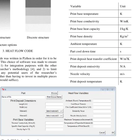
In order to satisfactorily simulate the heat flow through an FGM part, the code must have a number of input variables. The variables in Table 1 are those used in the simulation.
All variables are input via a graphical user interface (GUI), created by the researcher. This GUI automatically communicates with Abaqus. The GUI is shown in Figure 3.
Once the variables are input, the model is automatically created with the requirements specified. The model can then be checked by the user before the simulation is commenced.
Table 1: Variables used in simulation
Variable Unit
Print base temperature K
Print base conductivity W/mK
Print base heat capacity J/kg/K
Print base density Kg/m3
Ambient temperature K
Part cool down time s
Print deposit heat transfer coefficient W/m2K
Print deposit emissivity N/A
Nozzle velocity m/s
Print deposit temperature K
3.2 Steps that code undertakes
The simulation code uses several steps to create the FGM heat flow code. It first must set up the FGM material before it can begin developing the heat flow model. The main steps are:
1. Part division – the part is divided into many individual cells, each cell representing a single volume of deposited material. The cell size is a user-defined variable.
2. Apply FGMs – the graded materials (generated by the code) are allocated to the necessary cells.
[image:2.595.61.144.74.207.2]3. Print bed – a simulated print bed is built and attached to the part.
[image:2.595.110.534.104.551.2]4. Tool path – the tool path is decided. This must be modelled mathematically in order to represent the movements of the actual deposition head.
5. Deactivate cells – all cells are “turned off” in the simulation, leaving only the print bed active. The cells remain but have no effect on the heat transfer simulation.
6. Heat transfer conditions – radiation and convection conditions are created on all surfaces to represent the mechanisms occurring during additive manufacture. These surfaces include those cells which have been deactivated.
7. Heat material – all material is heated to the deposition temperature(s).
8. Reactivate cells – each segment is “turned on” during its own heat transfer step. The time the step takes is a function of the material volume within the cell. As each segment is reactivated it begins to have an effect on the heat transfer simulation.
9. Surface heat flux – the heat flux created due to the heat source is applied to all external faces.
10. Cooling – the part is cooled to the user-defined ambient temperature.
During step 8, the Python code requires Abaqus to run a user-defined subroutine. A subroutine allows the user to augment Abaqus commands in order to do task-specific functions. In this case, a mathematical model for the heat generated by the deposition head must be included.
3.3 Part division techniques
The part is divided using datum planes and cell partitioning. This is a two-stage process – the datum planes are made first, followed by the partitions. The spacing of the planes is user defined (via the GUI). Fig. 4 shows these two stages.
[image:3.595.304.549.455.635.2]Stage 1 – datum planes Stage 2 – partitions complete
Fig. 4: Stages of part division
3.4 Deactivating/Reactivating cells
To mimic the deposition of material during additive manufacture, cells of material are activated consecutively in the simulation. However, the model of the entire part must first be created – the simulation software cannot generate the part without any information. Once the part is created and divided, all cells must be deactivated, leaving only the print bed active. At this stage, the aim is to mimic a physical AM machine before deposition begins – no material is on the print bed. Once all cells are deactivated, each is reactivated consecutively as per the scanning strategy used by the AM machine. This consecutive reactivation aims to mimic the deposition of material in the physical AM machine.
3.5 Controlling nozzle velocity
The nozzle velocity is set by the user (via the GUI). As mentioned, the print deposits are activated sequentially following the raster scan path. The duration of time that each print deposit is heated for is a function of the nozzle velocity and the volume of material within each print deposit, as follows:
𝑡 = 𝑉𝐶 𝑉𝐷∗
𝐿 𝑠
where t is the duration of time that the print deposit is heated for (s), VC is the remaining volume of the current print deposit (m3), V
D is the total possible volume of the current
print deposit (m3), L is the length of the print deposit, and s is
the velocity of the nozzle (m/s).
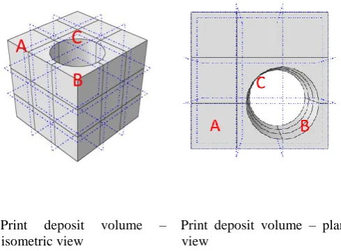
Print deposit volume – isometric view
Print deposit volume – plan view
Fig. 5: A description of the print deposit volume
Modifying the example part in Fig. 4 by cutting a hole in it (as seen in Fig. 5), VC and VD can be explained. Each print deposit is marked by the datum planes. Print deposit “A” completely fills the space bounded by the datum planes surrounding it. However, print deposits “B” and “C” do not.
Therefore, VC = VD in print deposit “A”, but VC < VD in print
[image:3.595.45.170.570.684.2]“A” will be heated for is therefore longer than the duration of time that print deposits “B” and “C” will be heated for.
3.6 Mathematical model of heat flow
The DFLUX subroutine is called every time the heat source moves between the single material deposition volumes. The path is determined by the mathematical model of the toolpath, as mentioned. The heat source is modelled as a Gaussian distribution. The equation used is:
𝑄(𝑟) = 𝑄𝐿
𝜋𝑟02𝑒 (1−𝑟2
𝑟02)
Where Q is the heat flux in terms of the radial distance from the centre of the laser beam, r, QL is the laser power, and r0 is the radius of the laser beam[7, 8].
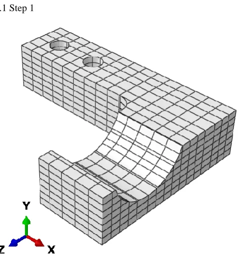
4. TEST PART
[image:4.595.307.530.72.268.2]The heat flow code was tested on a finger of a robotic arm gripper which picks and places specimens at 800°C. The contact area must withstand such temperatures. Other areas of the gripper do not have to withstand such temperatures, and therefore can be made from different material.
Fig. 6: Gripper finger - isometric view
[image:4.595.49.281.375.619.2]The gripper has two mirrored fingers that are actuated through an arc motion to enclose around a part. It is currently used to pick and place specimens to/from a forge for thermal processing. The form of one of the two mirrored fingers is shown in Fig. 6 and Fig. 7.
Fig. 7: Gripper finger - plan view
5. RESULTS
The results of several steps from section 3.2 are shown in this section.
Before step one, the model is first made. This can either be done in Abaqus, or imported using a suitable, cross-compatible 3D drawing format (.stp or .sat, for example). For this test piece, the part was imported as a .sat file.
5.1 Step 1
[image:4.595.310.549.417.676.2]5.2 Step 3
Fig. 9: Attaching print bed and applying material properties
[image:5.595.304.525.69.238.2]5.3 Step 5
Fig. 10: Deactivating the print deposits
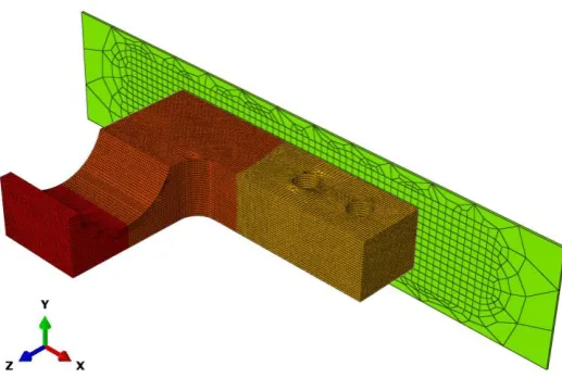
5.4 Step 8
Fig. 11: First print deposits reactivated
[image:5.595.46.213.301.436.2]Fig. 12: Further print deposits reactivated – cooling of deposits can be seen
Fig. 13: Further print deposits reactivated – further cooling present
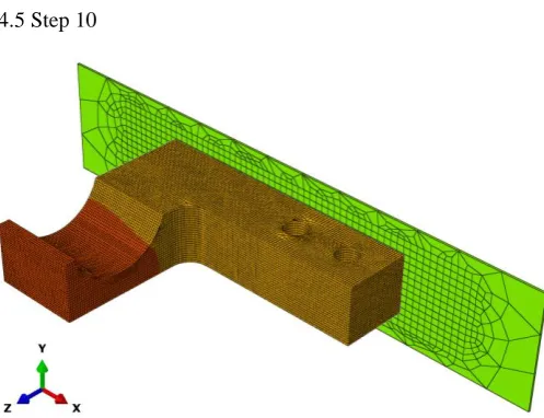
[image:5.595.305.556.309.479.2] [image:5.595.305.564.546.720.2]4.5 Step 10
[image:6.595.42.291.304.455.2]Fig. 15: During cooldown of part, once deposition is complete
Fig. 16: Heat flux after cooling
6. DISCUSSION
6.1 FGM positioning
The positioning of the FGM will alter, depending on the requirements of the part being produced. In this example part, the material is functionally graded between planes A and B in Fig. 6. After this point, the material remains that seen in the layer of cells immediately before plane B. In this example, Inconel 625 and stainless steel 316 L are used, due to their maturity with metallic additive manufacture. The Inconel grades decreasingly from plane B to plane A; the stainless steel grades decreasingly from plane A to plane B. The Inconel is chosen for its temperature resistant properties. The stainless steel has a lower temperature resistance, but also a lower density. The part is therefore lighter than it would be if made exclusively from the higher temperature-resistant Inconel 625.
6.2 Modelling material boundaries
The model currently assumes a perfect bond between each different material layer and no leeching of material or material properties. It is acknowledged that material
behaviour is complex during additive manufacture. This complexity is increased using FGMs. There are two areas of complexity:
1) The behaviour of bond layers between each FGM layer
2) The behaviour within each FGM layer
At present, no allocation is made for these bond layers. Work using UMAT (User MATerial) subroutines has shown promise for modelling other FGM surfaces [9]. This work will be incorporated into this simulation.
6.3 Purpose of print bed
As seen in Fig. 9, the print bed is attached in step 3. This allows the influence of heat flow and thermal conductivity from the print bed into the part to be observed. The print bed can be heated to any temperature chosen by the user. This is important, because heat flow across the part/print bed interface can cause warping and debonding issues, due to differences in temperature and coefficient of thermal expansion. Fig. 16 shows that there is a significant heat flux across the interface in this example.
6.4 Tool path modelling
The tool path is user-defined and modelled mathematically. This mathematical model must be chosen by the user and subsequently coded. Altering the tool path has a significant effect on mechanical properties [10] and surface finish [11] throughout the part. In this example a raster tool path was used.
6.5 Heat transfer mechanics
The heat transfer from the part into the surrounding atmosphere is modelled using both surface convection and surface radiation. The surfaces convection occurs uniformly, down to the ambient temperature of the surrounding atmosphere (user-controlled via GUI). The surface radiation mechanic is a function of the emissivity of the material (user-controlled via GUI), radiating heat uniformly from the surface to the ambient temperature of the surrounding atmosphere. Both conditions are applied to all external surfaces – in this case, the front face of the print bed and all external surfaces of the part.
6.6 Material heating
All material properties are applied to both the print bed and print deposits at this point during step 3. The first heat transfer step is also made – preheating all the print deposits. Fig. 10 in step 5 shows the print deposits once they have been deactivated. This occurs at the end of the second heat transfer step – preheating the print bed.
6.7 Creating moving heat source
The heat flow is tracked using a moving heat source (a surface heat flux). This is done using the DFLUX subroutine, as mentioned. The size of the laser spot is controllable (via the GUI), meaning the heat affected zone can be altered. The decision to heat an area is decided as a function of the laser spot size, the centre of the cell being heated, and the origin of the laser itself. If the centre of the cell falls within the radius of the laser spot, it will be heated. This heating is shown in the four figures of step 8 (Fig. 11, Fig. 12, Fig. 13 and Fig.
14). The temperature distribution is as expected – following the laser scan path while being influenced by residual heat in previous print deposits. This is the phase of the simulation where most of the heat transfer steps are undertaken – each print deposit is reactivated sequentially. In this simulation a raster scan tool path is used.
6.8 Cooling condition
The cooling step (step 10) allows the user to see where the heat flux effects after the additive manufacture has been completed. Fig. 16 shows that there are heat flux hotspots after cooling. These hotspots are in different areas compared to the temperature distribution in Fig. 15. It is these heat flux hot spots where the thermal residual stresses will be higher [12, 13]. If the residual stresses were extremely high at these points, redesign of the part could be considered.
6.9 Mesh Size
The mesh size is user-defined. The mesh in this model was chosen to ensure that each print deposit could model heat flow through itself. Each print deposit area has 750 elements within. As commonly acknowledged, a greater number of elements would produce a more realistic simulation at the trade-off of extra computing time/cost.
7. CONCLUSION
The results show that the heat flow code accurately mimics the movements of the print deposition head when the tool path is set. The temperature distribution is as expected with material heating and cooling occurring.
However, although both convection and radiation conditions are activated, the accuracy of the temperature outputs is difficult to determine without a physical demonstration for comparison - the temperatures seen in the simulation are assumed to be correlated to the temperatures seen on a physical part, but not exact representations due to the extreme
complexity of the additive manufacture process. For the simulation values to more accurately represent physical values, the understanding of the additive manufacturing process of multiple materials will need to be enhanced.
8. RELATED AND FUTURE WORK
Related to this work, and a possible validation avenue, is the use of embedded sensors. Embedded sensors are realisable with the use of AM – the build can be paused and the sensor(s) fitted. Additive manufacture has driven research into this field [14], increasing the accuracy while decreasing the size of such sensors. The task of the part being simulated and produced would decide the parameters that the sensor(s) would monitor, but could include strain [15], temperature [16], ultrasonic [17], pressure [18], electromagnetic [19], tactile [20], optical [21], chemical composition/presence [22, 23], force [24] and displacement [25] sensors. As mentioned, these sensors could aid validation of the simulation. MEMS (micro-electric mechanical systems) design techniques mean that sensors for certain parameters, such as pressure [26] and chemical presence [27] can now be produced at the micro-scale. In the gripper finger example, a strain sensor such as that used by Hermann et al. [28] could be embedded into the part. The measurements recorded on the sensor when the part is loaded under strain could then be compared to the outputs of the model. The accuracy of the simulated temperature distribution could also be checked using sensors – in this case, a surface coating similar to that implemented by Sauerbrunn et al. [29] could be appropriate, as it would record the surface temperatures of the gripper finger.
With respect to the simulation, future work will be aimed at increasing model accuracy. This will be done in two stages:
1) Make physical test specimens and measure actual mechanical properties. These will be fed into the model. It is assumed that embedded sensors will not be available – external strain gauges will be fitted.
2) Alter model at bond interface between each FGM using a UMAT subroutine. The UMAT subroutine can model specific material response. This will improve accuracy of the model.
9. REFERENCES
[1] D. Wang, Y. Yang, Z. Yi, and X. Su, “Research on the
fabricating quality optimization of the overhanging surface
in SLM process,” Int. J. Adv. Manuf. Technol., vol. 65, no.
9–12, pp. 1471–1484, 2013.
[2] J. Swanson, “Ansys.” Canonsburg, Pennsylvania, 2018.
[3] S. Littmarck and F. Saeidi, “COMSOL MultiPhysics.”
Burlington, MA, 2018.
[4] T. McMaster and X. Yan, “A methodology for design of
lightweight robotic arm links in harsh environments,” in
68th International Astronautical Congress, 2017, pp. 1–10.
[5] R. Gabbrielli, I. G. Turner, and C. R. Bowen,
“Development of modelling methods for materials to be
used as bone substitutes,” Key Eng. Mater., vol. 361–363
II, pp. 901–906, 2008.
of functionally gradient metals and metal-ceramic
composites: A review,” Acta Metallurgica Sinica (English
Letters), vol. 27, no. 5. pp. 825–838, 2014.
[7] O. Abdulghani, M. Sobih, A. Youssef, and A. El-Batahgy,
“Modeling and Simulation of Laser Assisted Turning of
Hard Steels,” Model. Numer. Simul. Mater. Sci., vol. 3, no.
4, pp. 106–113, 2013.
[8] P. R. De Freitas Teixeira, D. B. De Araújo, and L. A. B. Da
Cunha, “Study of the Gaussian distribution heat source model applied to numerical thermal simulations of tig
welding processes,” Cienc. y Eng. Sci. Eng. J., vol. 23, no.
1, pp. 115–122, 2014.
[9] W. G. Buttlar, G. H. Paulino, and S. H. Song, “Application
of graded finite elements for asphalt pavements,” J. Eng.
Mech., vol. 132, no. 3, pp. 240–249, 2006.
[10] P. Mognol, P. Muller, and J. Y. Hascoet, “Functionally
Graded Material (FGM) Parts: From Design To The
Manufacturing Simulation,” Proc. ASME 2012 11th Bienn.
Conf. Eng. Syst. Des. Anal., pp. 1–9, 2012.
[11] D. Ding, Z. (Stephen) Pan, D. Cuiuri, and H. Li, “A
tool-path generation strategy for wire and arc additive
manufacturing,” Int. J. Adv. Manuf. Technol., vol. 73, no. 1,
pp. 173–183, Jul. 2014.
[12] D. Deng and H. Murakawa, “Numerical simulation of
temperature field and residual stress in multi-pass welds in stainless steel pipe and comparison with experimental
measurements,” Comput. Mater. Sci., vol. 37, no. 3, pp.
269–277, Sep. 2006.
[13] O. Obeid, G. Alfano, H. Bahai, and H. Jouhara, “Numerical
simulation of thermal and residual stress fields induced by
lined pipe welding,” Therm. Sci. Eng. Prog., vol. 5, pp. 1–
14, Mar. 2018.
[14] Y. Xu, X. Wu, X. Guo, B. Kong, M. Zhang, X. Qian, S.
Mi, and W. Sun, The Boom in 3D-Printed Sensor
Technology, vol. 17, no. 6. 2017.
[15] M. Amjadi, Y. J. Yoon, and I. Park, “Ultra-stretchable and
skin-mountable strain sensors using carbon
nanotubes-Ecoflex nanocomposites,” Nanotechnology, vol. 26, no. 37,
2015.
[16] A. Wickberg, J. B. Mueller, Y. J. Mange, J. Fischer, T.
Nann, and M. Wegener, “Three-dimensional micro-printing of temperature sensors based on up-conversion
luminescence,” Appl. Phys. Lett., vol. 106, no. 13, 2015.
[17] D. I. Woodward, C. P. Purssell, D. R. Billson, D. A.
Hutchins, and S. J. Leigh, “Additively-manufactured
piezoelectric devices,” Phys. Status Solidi Appl. Mater.
Sci., vol. 212, no. 10, pp. 2107–2113, 2015.
[18] E. Suaste-Gómez, G. Rodríguez-Roldán, H. Reyes-Cruz,
and O. Terán-Jiménez, “Developing an ear prosthesis fabricated in polyvinylidene fluoride by a 3D printer with sensory intrinsic properties of pressure and temperature,”
Sensors (Switzerland), vol. 16, no. 3, 2016.
[19] B. Sanz-Izquierdo and E. A. Parker, “3-D printing of
elements in frequency selective arrays,” IEEE Trans.
Antennas Propag., vol. 62, no. 12, pp. 6060–6066, 2014.
[20] C. Shemelya, F. Cedillos, E. Aguilera, E. Maestas, J.
Ramos, D. Espalin, D. Muse, R. Wicker, and E.
MacDonald, “3D Printed Capacitive Sensors,” 2013 Ieee
Sensors, no. 3, pp. 1–4, 2013.
[21] T. Wolfer, P. Bollgruen, D. Mager, L. Overmeyer, and J. G.
Korvink, “Printing and preparation of integrated optical
waveguides for optronic sensor networks,” Mechatronics,
vol. 34, pp. 119–127, 2016.
[22] C. A. Mandon, L. J. Blum, and C. A. Marquette, “Adding
Biomolecular Recognition Capability to 3D Printed
Objects,” Anal. Chem., vol. 88, no. 21, pp. 10767–10772,
2016.
[23] K. Kadimisetty, I. M. Mosa, S. Malla, J. E.
Satterwhite-Warden, T. M. Kuhns, R. C. Faria, N. H. Lee, and J. F. Rusling, “3D-printed supercapacitor-powered
electrochemiluminescent protein immunoarray,” Biosens.
Bioelectron., vol. 77, pp. 188–193, 2016.
[24] S. B. Kesner and R. D. Howe, “Design principles for rapid
prototyping forces sensors using 3-D printing,”
IEEE/ASME Trans. Mechatronics, vol. 16, no. 5, pp. 866– 870, 2011.
[25] M. Bodnicki, P. Pakuła, and M. Zowade, “Miniature
displacement sensor,” in Advances in Intelligent Systems
and Computing, vol. 393, 2016, pp. 313–318.
[26] J. N. Palasagaram and R. Ramadoss, “MEMS-capacitive
pressure sensor fabricated using printed-circuit-processing
techniques,” IEEE Sens. J., vol. 6, no. 6, pp. 1374–1375,
2006.
[27] W. Lu, G. Jing, X. Bian, H. Yu, and T. Cui, “Micro
catalytic methane sensors based on 3D quartz structures with cone-shaped cavities etched by high-resolution
abrasive sand blasting,” Sensors Actuators, A Phys., vol.
242, pp. 9–17, 2016.
[28] J. Herrmann, K. H. Müller, T. Reda, G. R. Baxter, B.
Raguse, G. J. J. B. De Groot, R. Chai, M. Roberts, and L. Wieczorek, “Nanoparticle films as sensitive strain gauges,”
Appl. Phys. Lett., vol. 91, no. 18, 2007.
[29] E. Sauerbrunn, Y. Chen, J. Didion, M. Yu, E. Smela, and
H. A. Bruck, “Thermal imaging using polymer
nanocomposite temperature sensors,” Phys. Status Solidi