Fast Solar Radiation Pressure Modelling with Ray Tracing and Multiple reflections
Zhen Lia,∗, Marek Ziebarta, Santosh Bhattaraia, David Harrisona, Stuart Greyb
aUniversity College London, Gower Street, London WC1E 6BT, United Kingdom bUniversity of Strathclyde, 16 Richmond Street, Glasgow G11XQ, United Kingdom
Abstract
Physics based SRP (Solar Radiation Pressure) models using ray tracing methods are powerful tools when modelling the forces on complex real world space vehicles. Currently high resolution (1 mm) ray tracing with secondary intersections is done on high performance computers at UCL (University College London). This study introduces the BVH (Bounding Volume Hierarchy) into the ray tracing approach for physics based SRP modelling and makes it possible to run high resolution analysis on personal computers. The ray tracer is both general and efficient enough to cope with the complex shape of satellites and multiple reflections (three or more, with no upper limit). In this study, the traditional ray tracing technique is introduced in the first place and then the BVH is integrated into the ray tracing. Four aspects of the ray tracer were tested for investigating the performance including runtime, accuracy, the effects of multiple reflections and the effects of pixel array resolution.Test results in runtime on GPS IIR and Galileo IOV (In Orbit Validation) satellites show that the BVH can make the force model computation 30-50 times faster. The ray tracer has an absolute accuracy of several nanonewtons by comparing the test results for spheres and planes with the analytical computations. The multiple reflection effects are investigated both in the intersection number and acceleration on GPS IIR, Galileo IOV and Sentinel-1 spacecraft. Considering the number of intersections, the 3rd reflection can capture 99.12%, 99.14%, and 91.34% of the total reflections for GPS IIR, Galileo IOV satellite bus and the Sentinel-1 spacecraft respectively. In terms of the multiple reflection effects on the acceleration, the secondary reflection effect for Galileo IOV satellite and Sentinel-1 can reach 0.2 nm/s2and 0.4 nm/s2respectively. The error percentage in the accelerations magnitude results show that the 3rd reflection should be considered in order to make it less than 0.035%. The pixel array resolution tests show that the dimensions of the components have to be considered when choosing the spacing of the pixel in order not to miss some components of the satellite in ray tracing. This paper presents the first systematic and quantitative study of the secondary and higher order intersection effects. It shows conclusively the effect is non-negligible for certain classes of misson.
Keywords: SRP modelling; Fast Ray Tracing; Multiple-reflection; GPS IIR; Galileo IOV; Sentinel-1
1. Introduction
SRP ( Solar radiation pressure) has effects on all the artifi-cial satellites. It is the largest non-gravitational force for high altitude satellites. Take GNSS ( Global Navigation Satellite System) satellites as an example, SRP force will make them drift several hundred meters in one day (Springer et al,1999; Montenbruck and Gill,2005;Ziebart et al,2005). Thus it is very important to accurately model SRP for the sake of orbit quality.
Currently, the strategies for SRP modelling presented in the precise orbit determination community may be broadly divided into two categories. The first category is the empirical ap-proach. Triangular functions like sine and cosine are used in the along track, radial and cross track to absorb the un-modelled non-gravitational forces. This method has been applied to the orbit determination of many missions such as Sentinel-1 (Pe-ter et al,2017), Jason (Cerri et al,2010), HY-2A (Gao et al,
∗Corresponding author
Email addresses:hpulizhen@163.com(Zhen Li),
m.ziebart@ucl.ac.uk(Marek Ziebart),s.bhattarai@ucl.ac.uk (Santosh Bhattarai),david.harrison.14@ucl.ac.uk(David Harrison), stuart.grey@strath.ac.uk(Stuart Grey)
2015), GRACE (Gravity Recovery and Climate Experiment) (Kang et al,2006), GOCE (Gravity field and steady-state Ocean Circulation Explorer) (Casotto et al,2013) and GNSS satellites (Sibthorpe et al,2011;Arnold et al,2015). Although this ap-proach has been widely used by the community, it does have drawbacks. One aspect is that in the estimation of empirical parameters, there is a risk of mixing orbit dynamic parameters with other physical parameters such as earth orientation param-eters and geocentre (Meindl et al,2013). The other aspect is that the parameters in the empirical model have no clear phys-ical meaning which means it is less helpful for understanding what really happened to the satellites in space.
However, the complex shape and multiple materials of the satellite surfaces have to be considered in developing the high-fidelity SRP model. One way to deal with this problem is by using the ray tracing technique. For satellites that have dy-namic components such as the solar panels of GNSS satellites, the calculation of the dynamic components are separated for the efficiency of ray tracing though this may cause ignoring of shadowing effect from solar panels to the satellite bus. For the satellites that with all the components fixed such as Sentinel-1, the ray tracing can be applied directly.
The ray tracing technique accounts for the interactions be-tween each ray and satellite surfaces. But the number of rays can reach over 2.5×10⁷for satellites with a size of 5×5m2at only one direction of solar flux . Therefore, it is necessary to find a way to make this ray tracer more efficient in computation. Generally, this problem can be solved from two aspects. One aspect is to reduce the number of rays that needs to be calculated. The other aspect is to speed up the process of find-ing the intersections between rays and the spacecraft surfaces. Thus two questions will be produced with respect to the above two aspects. 1) How is the spacecraft geometry represented? 2) How to find the intersections as quick as possible? Regard-ing the first question, the satellite bus is represented by simple geometries that can be described by mathematical equations. The intersections can be calculated in an analytical way with this representation. As for the second question, there exits the first attempt to speed up the modelling computation by using block modelling approach (Sibthorpe,2006). In this study, the BVH (Bounding Volume Hierarchy) data structure is used in organising the components of the satellite bus. The essence of the BVH is a binary tree ( or K-Dimensional Tree ) that stores primitives in the scene where each node represents a bounding volume (Lauterbach et al,2009;Bittner et al,2015).
This paper firstly introduces the physical basis of SRP and is followed by the general ray tracing approach for SRP mod-elling. The representation of the satellite bus geometry and the intersection algorithm for each geometry are described along with the implementation of the ray tracer. Secondly, the BVH data structure is applied to the ray tracer to improve the perfor-mance. This BVH data structure reorganises the components of the satellite bus and speeds up the process of searching for the possible intersection components. Finally, the performance of the ray tracer is tested in four aspects, including absolute accu-racy, runtime, the effects of multiple reflections and the effects of pixel array resolution.
2. The physics of radiation pressure
The physical foundation is the basis for solar radiation pres-sure modelling. The theory of radiation prespres-sure was revealed by Maxwell as an assertion based on his theory of electromag-netism. The radiation pressure phenomenon was then validated in experiments by Nichols, Pyotr Nicholaievich Lebedev and Hull (Lebedev,1901;Nichols and Hull,1902,1903). Accord-ing to Maxwell’s theory, an electromagnetic wave carries mo-mentum which can be transferred to a reflecting or absorbing surface hit by the wave. The momentum change will generate
a force on the surface. By applying Einstein’s special theory of relativity and the theorem of impulse, the force generated by the electromagnetic wave is obtained. For a photon of frequencyf, the momentumpis given
p=h f
c (1)
[image:2.595.305.554.142.389.2]wherehis Planck’s constant.
Figure 1: This figure shows the force effects due to the incident ray on a plane
Figure1shows the process of reflection that happened on a plane. Assume there areNf photons at frequency f in the
inci-dent ray going through unit area at unit timedt,νfNf photons
are reflected. Within the reflected photons, there areµfνfNf
photons getting specularly reflected andνf(1−µf)Nf photons
getting diffusely reflected. For the diffuse reflection, assume the surface meets the requirement of Lambert assumption which means the intensity of the ray falls off by a factor ofcosθaway from the normal to the surface. The proportion of diffusely re-flected radiation that is emitted normal to surface is23 (Ziebart, 2004;Fliegel et al,1992). Applying the conservation of mo-mentum to the radiation flux and the surface:
Nfh f
c s=µfνf Nfh f
c r+ 2
3νf(1−µf) Nfh f
c n+∆pf (2)
where
sis the unit vector of incident ray.
ris the unit vector of specularly reflected direction. nis the unit normal vector of the surface.
∆pf is the momentum change due to the hit of photons of
fre-quency f per unit time.
Integrating over all the solar radiation spectrum ( assume the wavelength range is from 0 to∞), the momentum change can
be expressed:
∆p=
Z ∞
0
∆pfd f=
Z ∞
0
(s−µfνfr−2
3νf(1−µf)n) Nfh f
According to the theorem of impulse, the changes in momen-tum per unit time is actually the force.
F=∆p (4)
Given the power densityW ( photon flux multiply the energy per photon) in units of Watt·m−2, the reflectivityν and spec-ularity µ over the radiation spectrum, the area of the surface A and the incident angle θ. The power of the radiation that reaches the surface isWAcosθ. Therefore
F=WAcosθ
c
s−ν µr−2
3ν(1−µ)n
(5)
where the specularly reflected direction can be expressed
r=s−2(n·s)n
and
cosθ=−s·n
Equation (5) is the foundation of all the solar radiation pressure calculation. Fliegel et al(1992) andZiebart(2004) also gave out the analytical formula of direct solar radiation pressure in normal and shear components.
3. Spacecraft geometry representation and intersections
Usually the real world satellites have very complex shapes. However in the modelling of the satellite geometry, some sim-plifications and assumptions have to be made. Regarding the description of the satellite bus geometry, one way is to use a tessellation approach which represents complex geometry with a model consisting only of planar triangles (Grey et al,2017). However, this tessellation approach will introduce errors for the curved surfaces such as spheres, cylinders, parabolic dishes and so on. Therefore this study represents the real world satel-lite bus with components of simple geometries (Ziebart,2001, 2004). Such as polygons, discs, spheres, cylinders, cones and so on. These simple geometries can be described by rigorous mathematical equations and the intersections can be accurately computed.
In order to apply the BVH in ray tracing, all the components have to be surrounded by volumes, this can help to speed up the intersection searching process. In this study, the AABB (Axis Aligned Bounding Box) is used. The orientation of AABB is aligned to the three axes of the satellite BFS (Body Fixed Sys-tem ). The AABB for every component is stored as the mini-mum and maximini-mum coordinates in x, y and z. For every compo-nent, it also needs a Local Body System (LBS) to describe the geometry. The transformation matrix between the local body coordinate system and the satellite body fixed frame will be computed when building the geometry model.
The intersections between these geometries and the ray can be obtained by solving the simultaneous equations composed by the equation of ray and the equation of the geometry. Usu-ally the ray is expressed in the BFS with a start pointaand a unit direction vectord.
s=a+td (6)
wheretis the length of the ray.
The first step is to convert the ray from BFS to LBS. Once the intersection is computed and confirmed, it needs to be con-verted back to the BFS. The following section will discuss the solutions to the intersection problems for all the geometries.
Planar polygon & circle & ring
The intersection calculation for planar geometries requires two steps. The first step is to get the candidate intersection which is the intersection between the ray and the plane. The next step is to check if the candidate intersection is inside the shape. If the candidate intersection is outside the shape, it will not be ac-cepted as an intersection. In the local body coordinate system, the equation of a plane is
nTx=0 (7)
wherenis the normal vector of the plane,xis the coordinates of intersection point. Substituting the ray equation into this equa-tion, the parametertin the ray equation can be solved:
t=−n Ta
nTd (8)
Which means the distance between the start point of the ray and the candiate intersection is determined, thus the candidate inter-section point can be obtained. Once the candidate interinter-section is computed, the next step is to check if this candidate is inside the polygon or circle or the ring. This process will be different for the different geometries. For the polygons, this will involve the winding number theory in topology. The winding number of a closed curve in the plane around a given point is an in-teger representing the total number of times that curve travels counter clockwise around the point. If the winding number of the polygon for the candidate intersection is 0, the candidate is outside the polygon otherwise it is inside the polygon (Hor-mann and Agathos,2001). For circles, one only needs to check the distance between the centre of the circle and the candidate intersection. If the distance is less than the radius of the circle, then the candidate intersection gets accepted. It is similar for the planar ring, if the distance is greater than the radius of inner circle and less than the radius of external circle, the candidate gets accepted.
Sphere
In the local body frame of a sphere, the equation of a sphere can be described by
xTx=R2 (9)
whereRis the radius of the sphere.
Substituting the equation of the ray into this equation, a quadratic with respect to parametertis obtained
dTdt2+2dTat+aTa−R2=0 (10)
Table 1: The definition of local body frame and AABB for all the geometries
Geometry Representation Local body frame AABB
Polygon all vertices in counter clock-wise order
𝑥
𝑦 𝑧
𝑥
𝑦 𝑧
1(5)
3(7) 4(8)
2(6)
Circle radius, centre, two vertices on the circle in counter clockwise order
𝑥
𝑦 𝑧
𝑥
𝑦 𝑧
1(5)
2(6) 3(7) 4(8)
Ring centre, inner radius, outer radius, two vertices on the outer circle in counter clock-wise
𝑥
𝑦 𝑧
𝑥
𝑦 𝑧
1(5)
2(6) 3(7) 4(8)
Cone bottom vertex, top vertex,
radius, two vertices on the bottom circle in counter clockwise order
𝑥 𝑦
𝑧
𝑥 𝑦
1
2
3 4
5
6
7 8 𝑧
Sphere centre, radius
𝑥 𝑦
𝑧
𝑥 𝑦
𝑧
1
2
3 4
5
6 7
8
Cylinder centre, height, radius
𝑥 𝑦
𝑧
𝑥 𝑦
𝑧
1
2
3 4 5
6
the distance from the start of ray to the intersection, the smaller tmeans the first intersection of the ray. If the quadratic has only one solution, that means the ray is exactly tangent to the sphere.
Cylinder
The equation of a cylinder is
(
x2+y2=R2
0≤z≤h (11)
whereRis the radius of the cylinder andhis the height of the cylinder, i.e. the distance from centre of the bottom to centre of the top.
This set of equations does not include the bottom and top circles. In this study, the cylinder is open capped. Expand-ing the equation of ray into scalar form and combinExpand-ing them together, a quadratic with respect to parametertis obtained:
At2+Bt+C=0 (12)
whereA=x2d+yd2,B=2(xdxa+ydya),C=x2a+y2a−R2. It is
necessary to check the z component of the solution and make it meet the condition 0≤z≤h. If the above quadratic has two solutions, the smaller one would be the solution.
Cone
The equation of a conical surface is
(
z−h=−h R
p x2+y2
0≤z≤h (13)
whereRis the radius of the bottom circle,his the height of the cone. Combining this equation with the equation of the ray, it will generate a quadratic with respect to parametert
At2+Bt+C=0 (14)
whereA=z2d−h2
R2(y2d+x2d),B=2
zdza−hzd−h 2
R2(xdxa+ydya)
,
C=z2a+h2−2hz2a−h2
R2(x2a+y2a).
Check all the solutions to make sure the z coordinate of intersection meets the second equation of conical surface, i.e. 0≤z≤h. If the condition has been met, then a smaller will be chosen as the solution.
4. Traditional ray tracing for SRP modelling
The ray tracing approach can capture small components of the satellite geometry and it is easy to deal with complex shapes. In the modelling of solar radiation pressure, a pixel array is gen-erated with each pixel as the start point of the rays. The pixel array is placed in the direction of the sun with some distance away from the spacecraft (Ziebart,2001,2004; Ziebart et al, 2005;Tan et al,2016). In practice, the distance is set to make sure that the pixel array is outside of the spacecraft. The nor-mal to the pixel array is pointing to the origin of the body-fixed frame of the spacecraft. All the rays are parallel and they are all
in the normal direction of the pixel array. This is under the as-sumption that the sun is so far away from the earth orbit space-craft that all the rays are assumed to be parallel. Generally, the size of the pixel array is determined based on the size of the spacecraft, the requirement for this is that the pixel array has to fully cover the whole spacecraft, otherwise some rays may be missing. The general process of ray tracing includes three parts: 1) Input the satellite geometry description file. 2) Set up the pixel array. 3) For every ray starting from the pixel array, search all the geometry components to check the intersection. If there is an intersection for the ray, calculate the radiation force and then sum up. This intersection function will be called re-cursively to deal with the multiple reflection of the ray.
4.1. Construct the geometry model of the spacecraft
After obtaining the spacecraft information, the information is reorganized and expressed as the combination of basic ge-ometries described in table1. All the geometry information is written into a description file firstly. The content in the de-scription file includes not only the geometry information but also the optical properties such as reflectivity and specularity of each component. For the convenience of implementation in intersection check, there are two operations need to be done in the process of constructing the spacecraft geometry. The first is to establish the local body frame for every component in the description file according to the definition in table1. The ac-tual implementation about establishing the local body frame is to store the transformation parameters between the local body frame and the spacecraft body fixed frame. The transformation parameters include the coordinate of origin of the local body frame in spacecraft body fixed frame and the three unit vectors of the local body frame axis in spacecraft body fixed frame. The second is to build an AABB (Axis Aligned Bounding Box) for every component both in local body system and spacecraft body fixed frame. This AABB has two functions, one is help to determine the size of the pixel array, the other is to help speed up the intersection process using BVH algorithm.
4.2. Set up the pixel array
In the modelling of the solar radiation pressure, every di-rection of the solar radiation is simulated by a pixel array. The pixel array is placed atd0=100 meters away from the
space-craft in calculation. The main task for setting up the pixel array includes two aspects, the first is to determine the size of the pixel array and the second is to construct Pixel Array Coordi-nate system (PAC) that connects the pixel and the components in spacecraft body fixed frame. In the spacecraft body fixed frame, the direction of pixel array can be represented by a lon-gitude and a latitude as shown in Fig.2. The definition of PAC system is described as follows:
• 1) Rotate X axis around Z axis with angleλ in counter
clockwise order. Make sure that X axis of BFS lies in the projection of satellite-sun vector in XOY plane of BFS.
• 2) Rotate Z axis around Y axis with angle 3π
2 −ϕ in
• 3) Move the origin of BFS to the position of the sun.
Therefore the transformation between these two coordinate sys-tem is:
xPAC=R·xBFS+x0 (15)
where
R=
−sinϕcosλ −sinϕsinλ cosλ −sinλ cosλ 0
−cosϕcosλ −cosϕsinλ −sinϕ
and
x0= −d0cosϕcosλ −d0cosϕsinλ −d0sinλ
T
𝜆
𝜑
x
y
z
xPAC
yPAC
[image:6.595.39.301.127.506.2]z
PACFigure 2: This figure shows the definition of the Pixel Coordinate System (PAC) and the representation of latitudeϕand longitudeλof the sun in spacecraft BFS
Once the Pixel Array Coordinate system (PAC) is estab-lished, the size of the pixel array is calculated by converting the AABB of the whole spacecraft into PAC system, then the ranges of x and y coordinates in the PAC system are found. Be-cause the pixel array is aligned along the x and y axis of PAC, thus the length of the pixel array in x and y direction are com-puted according to the distance between the maximum and the minimum coordinates of the AABB respectively. The number of the pixels in each direction is calculated with the length di-vided by the spacing of the pixel array.
4.3. Intersections check and force calculation
For every ray emitted from the pixel array, it needs a loop to search all the components of the spacecraft to check the inter-sections. The intersection algorithm for individual component is described in section3. The ray may intersect multiple com-ponents, but only the closest intersection to the pixel is accepted as the real intersection. This is done by checking the distance
from the pixel to the candidate intersection. Once the intersec-tion is confirmed, the optical properties of the component and the normal to the surface at the intersection are also recorded. The force due to each ray is computed according to equation (5). If the pixel is small enough, the curved surface could be treated as a differential planeA. The relation betweenAand the area of the pixelA0is:
A0=Acosθ (16)
A0is computed according to the spacing of the pixel array. Thus
in equation (5), termAcosθshould be replaced byA0for every
intersected ray.
In the ray tracing, the Total Solar Irradiance (TSI) is set to be 1368 W·m−2(Hastings and Garrett,2004). TSI is actually varying with time and has a characteristics of the solar cycle. The variation should have impacts to the SRP modelling as TSI is an input to the ray tracing approach. However, we only focus on the ray tracing approach itself and assume all the inputs are correct and accurate as they should be.
The intensity of the ray is initially set to be 100% of the TSI. As for the multiple reflections, only the specular reflection is considered, thus the intensity of the reflected ray has to be re-duced byµ ν of the last intersected component (Ziebart,2001, 2004;Ziebart et al,2005). Ignoring the effects of diffusely re-flected radiation will introduce some mismodelling, resultant force caused by the secondary intersections will effectively be negligible (Ziebart,2001) because of the tendency for diffuse rays from many directions to cancel each other’ effects. In ad-dition, a similarly rigorous approach for considering the effects of the diffuse contribution in the multiple reflections would be impractical, as it would end up with exponential growth in the computation.
For the multiple specular reflections, the start point of the secondary reflected ray is the last intersection and the direction is the specularly reflected direction. After setting up the re-flected rays, the intersection process is called recursively till it strikes the maximum number of reflection.
5. Application of BVH in SRP modelling
BVH ( Bounding Volume Hierarchy) is a tree data structure on a set of geometric primitives, it has been widely used in colli-sion detection and ray tracing (Lauterbach et al,2009;G¨unther et al,2007;Sopin et al,2011;Bittner et al,2015). The essence of BVH is to organise the geometric objects that are wrapped in bounding volume in a binary tree. It recursively partitions the bounding volume by planes and stores the children in the binary tree.
The application of BVH includes the construction of the BVH tree and traverse of the tree. The details of building the BVH with the spacecraft geometries and searching for the in-tersections are discussed in the following sections.
5.1. Construction of BVH for the spacecraft
root node of the BVH is the spacecraft AABB. The establish-ment of the BVH tree is the process of partitioning the AABB into different levels of sub-AABB and store them into a binary tree. For each AABB, the geometric centre is chosen as its ref-erence point. The key factor that affects the efficiency of a BVH is how to choose the partition plane. There are many algorithms of choosing the partition plane in an optimized way (Sopin et al, 2011). Because how to improve the efficiency of BVH in ray tracing is not the focus of this study, a widely used approach is applied in this study. This approach is in two steps. The first step is to choose the longest axis (this axis can either be x, y or z axis) of the AABB. Step two is to choose the partition plane and make it go through the middle point of the longest axis. For ev-ery partition, the AABB is divided into two sub-volumes. The steps of building the BVH are as follows:
• 1) Let the root node be the AABB of the whole spacecraft geometry.
• 2) Choose the partition plane of the root node.
• 3) Loop over all the geometry components, if the refer-ence point of the AABB for the geometry lies on the left side of the partition plane, the component will be stored in the left child, otherwise the component will be sent to the right child.
• 4) Repeat step1 to step3 for both the left and right child till the number of geometry of the children is 1. The nodes that have only one component inside are treated as leaves.
5.2. Traverse and intersection check
The traverse of the BVH tree is the key part of searching the intersection. Because all the nodes of the BVH tree are surrounded by AABBs, if the ray misses the AABB, the ray will not hit any components inside the AABB. If the ray hits the AABB of that node, all the children of that node should be checked until it reaches the leaves of the tree. For the leaves of the tree, because they are one of the simple geometries de-scribed in the previous sections, the intersection algorithm for them can be applied. The closest intersection to the start of the ray is the final solution. The steps for traversing the BVH tree are as follows:
• 1) Start from the root of the BVH tree, if the ray hits the AABB, then check the left child and the right child. Otherwise, the ray will not hit any part of the spacecraft.
• 2) Repeat the above step till it reaches the leaves. The intersection algorithm for the leaves will be executed If the ray hits the leaf geometry, the distance from this in-tersection to the start of the ray is record.
• 3) Finally, the real intersection is the one that is closest to the start of the ray.
Similarly, this traverse algorithm is also designed to be re-cursive. This traverse algorithm will return false if there is no
intersection, otherwise it will return true. The optical proper-ties, normal vector to the intersected surface and coordinates of intersection will be returned as well. In this traverse process, one key part is to check the intersection of a ray and the bound-ing box. This has to be ran for so many times that it is very important to make it fast. This study applied an efficient and robust ray-box intersection algorithm (Williams et al,2003) .
6. Test and validation
In this section, the processes for verifying the input (i.e. the spacecraft geometrical model) and testing the performance of the algorithm are described. Quality control checks are carried out to verify the geometry and to confirm that the ray-tracer de-tects the spacecraft in a correct way. To assess the performance of the ray tracer, a number of tests were done to investigate var-ious aspects. These include tests to examine the absolute accu-racy of the force computations and tests to determine the impact of pixel-array spacing on the accuracy of the result. Also, the impact of introducing BVH into the ray-tracing method is anal-ysed using runtime (with and without BVH) comparison tests. Finally, the impact of neglecting the effects of reflected radia-tion, considering up to 10 reflections, are assessed using models for the GPS IIR and Galileo IOV satellite bus, and a model for the Sentinel-1 spacecraft, as shown in Fig.3.
[image:7.595.306.578.543.619.2]The spacecraft models are produced using data from a vari-ety of sources (e.g. design drawings, CAD models). This data is used to represent the surface geometry of the spacecraft using the geometric primitives described in Table1. The information on the spacecraft models is shown in Table2. The mass of the satellites may be varying depends on different satellites and op-eration state. The information of GPS IIR satellite can be found fromZiebart et al(2003). For Galileo IOV satellite, we use the data published at European GNSS Service Centre (European Global Navigation Satellite Systems Agency,2017). The mass of Sentinel-1 satellite is obtained fromPeter et al(2017).
Table 2: The information on the spacecraft model
Items GPS IIR Galileo IOV Sentinel-1
mass 1086.451 kg 696.815 kg 2158.777 kg
# of compo-nents
182 590 4081
min. dimen-sion
Figure 3: Visualisation of the spacecraft models used in this study: Galileo IOV bus (upper-left), GPS IIR bus (lower-left) and Sentinel-1 (right). For each model, the coordinate systems shown represent the spacecraft BFS x (red), y (green) and z (blue) axes.
6.1. Quality control checks of the spacecraft models
Two simple quality control (QC) checks are used to verify the spacecraft models. First, the spacecraft model file is exam-ined in a 3D-viewer, where it is possible to rotate around the spacecraft model to assess the data for errors in the geometry. The models for the Galileo IOV bus, GPS IIR bus and Sentinel-1 spacecraft, as seen in the spacecraft model viewer are shown in Fig. 3. The second QC check is a coarse intersection test that is used to confirm that the ray-tracing software is correctly detecting the spacecraft surface. In Fig. 4, the results of two coarse intersection tests on the Galileo IOV bus model, at pixel array spacings of 1 dm (left) and 1 cm (right), are shown. In the 3D-viewer, intersections are shown as red dots. With the 1 cm intersection test, it is possible to show the effectiveness of the ray-tracing software in capturing the effects of self-shadowing – note the shadows cast by the cylinders of the SAR (Search And Rescue) antenna in Fig.4(right).
self-shadow
Figure 4: 3D visualisation of the results of intersection tests on the Galileo IOV bus model with pixel array spacing at 1 dm (left) and 1 cm (right). Note that on the right figure, the shadows cast by the cylinders of the SAR antenna can be clearly seen.
6.2. Testing the absolute accuracy of the algorithm
Two test objects, a sphere and a planar surface, are used to assess the absolute accuracy of the proposed technique. For these objects, it is possible to evaluate the accelerations using analytical methods. Therefore, it is possible to use the ana-lytical results as a baseline for evaluating the accuracy of the
proposed, computational approach. In these tests, the pixel ar-ray spacing is set at 1 mm and the mass of the test objects are set at 1 kg. Other key parameters in these tests are summarised in Table3.
For both objects, the pixel array moves in the YOZ plane, scanning the objects from the +y axis (θ =0) to the -y axis
(θ=180), in 1-degree increments, as shown in Fig. 5, where θ is the angle between the anti-ray direction and the +y axis.
With this scanning strategy, the x component of the incoming rays are always equal to zero, while the y and z components are symmetric about the XZ plane.
Table 3: The key parameters for setting up the absolute accuracy test.
Items Values
solar constant 1368 W·m−2
reflectivity 0.7
specularity 0.4
resolution 1 mm
area of the plane 4.0 m2 radius of the sphere 1.0 m
mass 1.0 kg
𝑥
𝑦 𝑧
𝑠
(a) sphere test
𝑥
𝑦 𝑧
𝑠
[image:8.595.319.546.242.484.2](b) plane test
Figure 5: The test cases for the sphere and plane, the sun is scanning from the +y to -y.
Plane test
[image:8.595.46.282.519.625.2]0
20 40 60 80 100 120 140 160 180
Angle [degree]
30000
25000
20000
15000
10000
5000
0
5000
Ac
c [
nm
s
2
]
[image:9.595.40.287.87.214.2]x
y
z
Figure 6: The force of the plane test
0
20
40
60
80 100 120 140 160 180
Angle [degree]
8
6
4
2
0
2
4
6
8
Ac
c [
nm
s
2
]
avg = 0.14
[image:9.595.311.555.88.212.2]std = 3.19
Difference in magnitude
Figure 7: The difference between the ray tracer and analytical solution for the plane
Sphere test
As for the sphere, equation (5) is applied to the differential area and is integrated around the hemi-sphere. The integration gives out the analytical formula of the SRP force for spheres
F=WπR 2
c
1+4
9ν− 4 9ν µ
s (17)
Figure8shows the acceleration from the ray tracer in the sphere test and the difference in magnitude between ray tracer and the analytical solution is shown in Fig.9. The average value of the difference is -0.046 nm/s2and the standard deviation is 0.112 nm/s2.
0
20 40 60 80 100 120 140 160 180
Angle [degree]
15000
10000
5000
0
5000
10000
15000
Ac
c [
nm
s
2
]
x
y
z
Figure 8: The acceleration from the sphere test
0
20 40 60 80 100 120 140 160 180
Angle [degree]
0.3
0.2
0.1
0.0
0.1
0.2
0.3
Ac
c [
nm
s
2
]
avg = -0.05
std = 0.11
Difference in magnitude
Figure 9: The difference between the ray tracer and analytical solution for the sphere
Note that the standard deviation of the differences is about 30 times smaller in the sphere test than it is in the planar surface test. This is because of errors in the pixel-array based technique that occur at the edges of the geometry. For instance, in the case of the sphere, which has a radius of 1 m in this test, the edge of the sphere is a circle of circumference 2π m, and as the ra-diation source (simulated by the pixel array) pans across the sphere, this is nearly constant. On the other hand, for the planar surface, the perimeter of the edge of the geometry varies as the pixel array pans across theθ=0−180 range. Therefore, when the radiation source is lower, as the pixel array is projected onto the cross-section of the planar surface, the perimeter/area ratio increases, and this increases the relative error at the edges. This link between the the linear dimensions of the pixel array grid cells and the magnitude of the errors in the ray-tracing tech-nique are explored further in the next section.
6.3. The effects of the pixel array resolution
This is to test the effects of different sizes of the pixel in the ray tracing. In general, smaller pixel size will lead to higher modelling accuracy. In this test, 4 different resolutions includ-ing 1 dm, 1cm, 1mm and 0.1mm are chosen. We take 0.1 mm resolution as the baseline, the difference in force are calculated between the baseline and other resolutions. The GPS IIR and Galileo IOV satellites are tested in the yaw steering attitude (Montenbruck et al,2015a) while Sentinel-1 satellite is tested in the roll steering attitude (Peter et al,2017). The magnitude of the acceleration are shown in Fig.10for the bus of GPS IIR, Galileo IOV and the whole spacecraft of Sentinel-1.
[image:9.595.41.288.257.390.2] [image:9.595.40.286.609.731.2]the pixel resolution, the pixel resolution for the ray tracer should be smaller in order to capture all the geometrical information.
The relative accuracy for different pixel spacing can be cal-culated by dividing the standard deviation by the average ac-celeration. The average accelerations for GPS IIR bus, Galileo IOV bus and the Sentinel-1 spacecraft are 20.576 nm·s−2, 28.110
nm·s−2, and 81.381 nm·s−2 as shown in Fig. 10. The rela-tive accuracy for different pixel resolutions is shown in Table 4. The relative accuracy is mainly driven by the pixel spacing, the relative accuracy of 1 dm pixel spacing is about 1.7% and it gets almost 10 times smaller for 1 cm and so forth for 1 mm spacing. This is because as the pixel spacing gets smaller, the sampling error for the cross-section area gets smaller and the error in the cross-section has linear impact to the SRP acceler-ation (See equacceler-ation5). For most of the satellites, a resolution of 1 mm should be good enough for the SRP modelling. Thus in the following multiple reflection test, the spacing of the pixel array is set to be 1 mm.
90
60
30
0
30
60
90
Latitude of the sun in body fixed frame [degree]
20
40
60
80
100
Ac
c [
nm
s
2
]
[image:10.595.309.556.87.216.2]GPS IIR
Galileo IOV
Sentinel-1
[image:10.595.304.552.88.535.2]Figure 10: The errors with 1mm pixel resolution
Table 4: The error statistics of different resolutions [unit:nm·s−2]
Resolution 1 dm 1 cm 1 mm
Galileo IOV Avg. -0.711E-2 -0.815E-3 3.706E-5
GPS IIR Avg. -0.273 -0.091 0.755E-3
Sentinel-1 Avg. -0.281 0.032 -0.641E-3
Galileo IOV Std. 0.495 0.039 0.004
GPS IIR Std. 0.335 0.038 0.002
Sentinel-1 Std. 1.416 0.139 0.013
Galileo IOV rel. 1.761% 0.139% 0.014%
GPS IIR rel. 1.628% 0.185% 0.010%
Sentinel-1 rel. 1.739% 0.171% 0.016%
90
60
30
0
30
60
90
Latitude of the sun in body fixed frame [degree]
4
2
0
2
Ac
c [
nm
s
2
]
Galileo IOV
GPS IIR
Sentinel-1
Figure 11: The errors with 1dm pixel resolution
90
60
30
0
30
60
90
Latitude of the sun in body fixed frame [degree]
0.3
0.2
0.1
0.0
0.1
0.2
0.3
0.4
0.5
Ac
c [
nm
s
2
]
Galileo IOV
GPS IIR
Sentinel-1
Figure 12: The errors with 1cm pixel resolution
90
60
30
0
30
60
90
Latitude of the sun in body fixed frame [degree]
0.03
0.02
0.01
0.00
0.01
0.02
0.03
Ac
c [
nm
s
2
]
[image:10.595.41.287.316.440.2]Galileo IOV
GPS IIR
Sentinel-1
Figure 13: The errors with 1mm pixel resolution
6.4. Speedup test
[image:10.595.307.555.439.569.2] [image:10.595.42.283.503.627.2]algorithm is about 30-50 times faster than the UCL raw soft-ware.
Table 5: The speedup test for a GPS IIR satellite bus
Method UCL raw no BVH with BVH
1 dm (ms) 106.78 53.52 2.97
1 cm (s) 9.27 5.38 0.32
1 mm (min) 14.45 8.79 0.46
[image:11.595.57.268.130.195.2]avg. speedup 1.0 1.78 32.69
Table 6: The speedup test for one Galileo IOV satellite bus
Method UCL raw no BVH with BVH
1 dm (ms) 75.601 35.45 1.11
1 cm (s) 5.30 3.30 0.10
1 mm (min) 8.09 8.79 0.15
avg. speedup 1.0 1.75 59.39
6.5. Multiple reflection test
In the solar radiation pressure modelling for GLONASS satel-lites, the secondary reflection effects in the force can cause 0.1 m error in the along-tack after 12 hours (Ziebart,2001). The 1st reflection is defined as the the ray hit and bounce off but not any further intersections. Thus the secondary reflection ef-fect is the error due to omitting 2nd, 3rd etc. intersections. In this study, we take the 10-reflection as a base line, the effects of multiple reflections are investigated in two aspects, one is the proportion of intersection number for multiple reflections over the base line, the other is the difference in acceleration between multiple reflections and the base line.
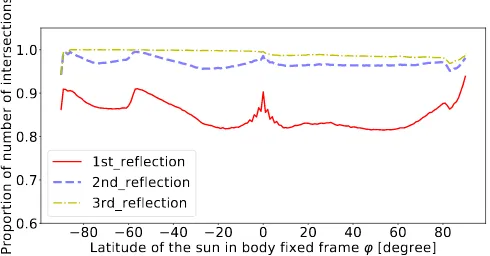
Figure14, Fig.15, and Fig.16show the proportion of inter-section number with respect to the reflection number for GPS IIR, Galileo IOV and Sentinel-1 satellites respectively. As Fig. 17and Table7show, the primary rays can only capture about 85%, 91%, and 84% of the total rays for GPS IIR, Galileo IOV satellite bus and Sentinel-1 separately. The secondary reflec-tion can capture over 96% while the third reflecreflec-tion can capture over 99% for GPS IIR and Galileo IOV satellite bus. Because of the complex shape of Sentinel-1, even the third reflection can just capture around 91%. However, this does not mean the ac-curacy in the acceleration. The reduction of the energy of the reflected rays make the contribution of multiple reflected rays to the acceleration gets smaller and smaller.
The multiple reflection effects of Sentinel-1 spacecraft would be obvious due to its large SAR (Synthetic Aperture Radar) an-tenna and the big solar panels, see Fig. 3. The difference in acceleration for GPS IIR (bus only), Galileo IOV (bus only) and Sentinel1 (whole spacecraft) between the 1st, 2nd, 3rd re-flection and the base line are shown in Fig. 18, Fig. 19, Fig. 20. In terms of the percentage in acceleration magnitude due to multiple reflections, Galileo IOV satellite bus gets the largest (around 1%) among the three space crafts due to its large area to mass ratio. Figure21shows the error percentage of acceler-ation magnitude for 1st, 2nd and 3rd reflections.
The errors in acceleration due to the 1st reflection can reach to 0.2 nm/s2 and 0.4 nm/s2 for Galileo IOV and Sentinel-1
Table 7: This table shows the average proportion of intersections w.r.t reflection number
# of reflection GPS IIR Galileo IOV Sentinel-1
1 84.988% 91.221% 84.683%
2 96.935% 98.123% 89.291%
3 99.127% 99.137% 91.341%
4 99.574% 99.534% 92.941%
5 99.755% 99.730% 94.321%
6 99.828% 99.842% 95.586%
7 99.897% 99.919% 96.772%
8 99.915% 99.963% 97.898%
9 99.940% 99.984% 98.971%
10 100% 100% 100%
separately. For the 2nd and 3rd reflections, the errors get 2 or 3 order of magnitude smaller. In terms of the percentage error in acceleration magnitude, the percentage can reach 1% , 0.1% and 0.035% for 1st, 2nd and 3rd reflections.
80
60
40
20 0
20
40
60
80
Latitude of the sun in body fixed frame [degree]
0.6
0.7
0.8
0.9
1.0
Proportion of number of intersections
[image:11.595.58.267.233.296.2]1st_reflection
2nd_reflection
3rd_reflection
Figure 14: The difference in the proportion of number of intersection between different number of reflection for GPS IIR satellite bus
80
60
40
20 0
20
40
60
80
Latitude of the sun in body fixed frame [degree]
0.80
0.85
0.90
0.95
1.00
1.05
Proportion of number of intersections
1st_reflection
2nd_reflection
3rd_reflection
Figure 15: The difference in the proportion of number of intersection between different number of reflection for Galileo IOV satellite bus
[image:11.595.310.555.321.449.2] [image:11.595.309.556.506.635.2]ge-80
60
40
20 0
20
40
60
80
Latitude of the sun in body fixed frame [degree]
0.5
0.6
0.7
0.8
0.9
1.0
Proportion of number of intersections
[image:12.595.40.287.107.234.2]1st_reflection
2nd_reflection
3rd_reflection
Figure 16: The difference in the proportion of number of intersection between different number of reflection for Sentinel-1 spacecraft
1
2
3
4
5
6
7
8
9
10
Number of reflections
0.84
0.86
0.88
0.90
0.92
0.94
0.96
0.98
1.00
Proportion of number of intersections
[image:12.595.311.552.144.335.2]GPS IIR
Galileo IOV
Sentinel-1
Figure 17: The average proportion of number of intersection for different num-ber of reflection
0.20
0.15
0.10
0.05
0.00
x [
nm
s
2
]
GPS IIR
Galileo IOV
Sentinel-1
0.4
0.3
0.2
0.1
0.0
0.1
y [
nm
s
2
]
90
60
30
0
30
60
90
The Latitude of the sun in Body Fixed Frame [degree]
0.4
0.3
0.2
0.1
0.0
0.1
0.2
z
[n
m
s
2
]
Figure 18: The errors in acceleration for the 1st reflection
1.4 1.2 1.0 0.8 0.6 0.4 0.2 0.0 0.2
x [
nm
s
2
]
1e 2
GPS IIR
Galileo IOV
Sentinel-1
2.0
1.5
1.0
0.5
0.0
0.5
1.0
y [
nm
s
2
]
1e 2
90
60
30
0
30
60
90
The Latitude of the sun in Body Fixed Frame [degree]
1.0
0.5
0.0
0.5
1.0
1.5
z
[n
m
s
[image:12.595.41.286.313.441.2]2
]
1e 2
Figure 19: The errors in acceleration for the 2nd reflection
54
32
10
1
x [
nm
s
2
]
1e 3
GPS IIR
Galileo IOV
Sentinel-1
3.5
3.0
2.5
2.0
1.5
1.0
0.5
0.0
0.5
y [
nm
s
2
]
1e 3
90
60
30
0
30
60
90
The Latitude of the sun in Body Fixed Frame [degree]
0.50
0.25
0.00
0.25
0.50
0.75
1.00
1.25
z
[n
m
s
2
]
1e 2
[image:12.595.311.552.495.678.2] [image:12.595.43.284.527.716.2]1.0
0.8
0.6
0.4
0.2
0.0
1st ref. [%]
GPS IIR
Galileo IOV
Sentinel-1
0.08
0.06
0.04
0.02
0.00
0.02
2nd ref. [%]
90
60
30
0
30
60
90
The Latitude of the sun in Body Fixed Frame [degree]
3.0
2.5
2.0
1.5
1.0
0.5
0.0
0.5
3rd ref. [%]
[image:13.595.42.285.87.276.2]1e 2
Figure 21: The percentage of errors due to 1st, 2nd and 3rd reflections for GPS IIR, Galileo IOV and Sentinel-1 spacecraft
ometrical model and the satellite mass ) to the ray tracing ap-proach are encouraged to be made more accurate.
7. Conclusion
This research starts from the physical basis of radiation force, then a ray tracing based high-fidelity radiation pressure mod-elling technique is followed. Thereafter, the BVH data structure is applied to the ray tracing process and it makes the ray tracing process run faster. The tests focus on 4 aspects including the ac-curacy of the ray tracing technique for radiation pressure mod-elling, the speed up efficiency of the BVH on radiation pressure modelling, the effects of multiple reflections, the effects of the pixel resolution.
The accuracy tests on a plane and a sphere show that this ray tracing technique can reach an accuracy of about several nano meter per square seconds with a pixel array resolution of 1 mm. In practice, this accuracy could be affected by the relative ratio of the actual size of the spacecraft over the pixel array resolu-tion. In addition, in the test of the pixel array resolution for GPS IIR spacecraft, a bias has been found for the resolution of 1 dm and 1cm. The reason for this is that there are many cylindrical antennas that have a radius of around 1 cm. A resolution of 1cm in the pixel array may cause a large sum of rays to miss those components. The effects can be seen clearly in Fig. 12. In or-der to balance between the accuracy and the computation time, a proper resolution of the pixel array has to be chosen according to the details of the spacecraft.
The test results on multiple reflections for GPS IIR and Galileo IOV satellites show that the first three reflections for each ray can capture over 99% of the total intersections. Though the first three reflections can only capture around 90% of the to-tal intersections for Sentinel-1, the contribution in acceleration due to multiple reflections gets smaller and smaller as the in-crease of the reflection number due to the reduced energy of the reflected rays. The tests on the effects of multiple reflections in
acceleration show that the secondary intersection effect is non-negligible for both Galileo IOV satellite and Sentinel-1 space-craft. The magnitude of acceleration due to secondary intersec-tion can reach 0.2 nm/s2 and 0.4 nm/s2 for Galileo IOV and
Sentinel-1 spacecraft separately. Considering the 3rd intersec-tion can make the error percentage less than 0.035%. Thus in the modelling of solar radiation pressure with ray tracing tech-nique, the 3rd reflection should be considered. It is the first time to do systematic and quantitative study on the secondary and higher order intersection effect and it shows conclusively the effect is non-negligible for certain classes of mission.
Despite the ray tracing approach itself can reach high accu-racy in SRP modelling, the accuaccu-racy is limited by the inputs to the approach. Such as the variation of the TSI, the optical prop-erties, the geometrical model. The current input data for high precision SRP modelling is not satisfied to some extent. There-fore, the measurements of the surface optical properties of the materials and the operational mass of the satellite are encour-aged to be make public.
Acknowledgements
This work is jointly funded by University College London and China Scholarship Council. Thanks for collegue who worked on the UCL (University College London) Solar Radiation Pres-sure Modelling software in the past and present.
References
Arnold D, Meindl M, Beutler G, Dach R, Schaer S, Lutz S, Prange L, So´snica K, Mervart L, J¨aggi A (2015) CODE’s new solar radiation pressure model for GNSS orbit determination. Journal of Geodesy 89(8):775–791, DOI 10.1007/s00190-015-0814-4
Bittner J, Hapala M, Havran V (2015) Incremental BVH construction for ray tracing. Computers and Graphics (Pergamon) 47:135–144, DOI 10.1016/j. cag.2014.12.001
Casotto S, Gini F, Panzetta F, Bardella M (2013) Fully dynamic approach for GOCE precise orbit determination. Bollettino di Geofisica Teorica ed Ap-plicata 54(4):367–384, DOI 10.4430/bgta0108
Cerri L, Berthias JP, Bertiger WI, Haines BJ, Lemoine FG, Mercier F, Ries JC, Willis P, Zelensky NP, Ziebart M (2010) Precision orbit determination stan-dards for the Jason series of altimeter missions. Marine Geodesy 33(SUPPL. 1):379–418, DOI 10.1080/01490419.2010.488966
European Global Navigation Satellite Systems Agency (2017) Galileo Satellite Metadata. URL https://www.gsc-europa.eu/ galileo-gsc-overview/system
Fliegel HF, Gallini TE, Swift ER (1992) Global Positioning System Radiation Force Model for geodetic applications. Journal of Geophysical Research 97(B1):559, DOI 10.1029/91JB02564
Gao F, Peng B, Zhang Y, Evariste NH, Liu J, Wang X, Zhong M, Lin M, Wang N, Chen R, Xu H (2015) Analysis of HY2A precise orbit determination using DORIS. Advances in Space Research 55(5):1394–1404, DOI 10.1016/ j.asr.2014.11.032
Grey S, Marchand R, Ziebart M, Omar R (2017) Sunlight Illumination Mod-els for Spacecraft Surface Charging. IEEE Transactions on Plasma Science 45(8):1898–1905, DOI 10.1109/TPS.2017.2703984
G¨unther J, Popov S, Seidel HP, Slusallek P (2007) Realtime ray tracing on GPU with BVH-based packet traversal. In: IEEE/ EG Symposium on Interactive Ray Tracing 2007 Proceedings, IRT, pp 113–118, DOI 10.1109/RT.2007. 4342598
Hormann K, Agathos A (2001) The point in polygon problem for arbitrary poly-gons. Computational Geometry: Theory and Applications 20(3):131–144, DOI 10.1016/S0925-7721(01)00012-8
Kang Z, Tapley B, Bettadpur S, Ries J, Nagel P, Pastor R (2006) Precise or-bit determination for the GRACE mission using only GPS data. Journal of Geodesy 80(6):322–331, DOI 10.1007/s00190-006-0073-5
Lauterbach C, Garland M, Sengupta S, Luebke D, Manocha D (2009) Fast BVH Construction on GPUs. Computer Graphics Forum 28(2):375–384, DOI 10.1111/j.1467-8659.2009.01377.x
Lebedev PN (1901) Experimental Examination of Light Pressure. Annalen der Physik 6(433):1–26, DOI 10.1002/andp.19013111102
Meindl M, Beutler G, Thaller D, Dach R, Jaggi A (2013) Geocenter coordinates estimated from GNSS data as viewed by perturbation theory. Advances in Space Research 51(7):1047–1064, DOI 10.1016/j.asr.2012.10.026 Montenbruck O, Gill E (2005) Satellite Orbits Models, Methods and
Ap-plications, corrected edn. Springer Berlin Heidelberg, Berlin, Heidelberg, DOI 10.1007/978-3-642-58351-3, URLhttp://link.springer.com/ 10.1007/978-3-642-58351-3
Montenbruck O, Schmid R, Mercier F, Steigenberger P, Noll C, Fatkulin R, Kogure S, Ganeshan AS (2015a) GNSS satellite geometry and attitude mod-els. Advances in Space Research 56(6):1015–1029, DOI 10.1016/j.asr.2015. 06.019, URLhttp://dx.doi.org/10.1016/j.asr.2015.06.019
Montenbruck O, Steigenberger P, Hugentobler U (2015b) Enhanced solar radia-tion pressure modeling for Galileo satellites. Journal of Geodesy 89(3):283– 297, DOI 10.1007/s00190-014-0774-0
Nichols E, Hull G (1902) Pressure due to light and heat radiation. The Astro-physical Journal 15:62
Nichols EF, Hull GF (1903) The Pressure Due to Radiation. Proceedings of the American Academy of Arts and Sciences 38(20):559, DOI 10.2307/ 20021808
Peter H, J¨aggi A, Fern´andez J, Escobar D, Ayuga F, Arnold D, Wermuth M, Hackel S, Otten M, Simons W, Visser P, Hugentobler U, F´em´enias P (2017) Sentinel-1A First precise orbit determination results. Advances in Space Research 60(5):879–892, DOI 10.1016/j.asr.2017.05.034
Sibthorpe A, Bertiger W, Desai SD, Haines B, Harvey N, Weiss JP (2011) An evaluation of solar radiation pressure strategies for the GPS constellation. Journal of Geodesy 85(8):505–517, DOI 10.1007/s00190-011-0450-6 Sibthorpe AJ (2006) Precision Non-Conservative Force Modelling For Low
Earth Orbiting Spacecraft. PhD thesis, University College London Solano CJR (2014) Impact of non-conservative force modeling on GNSS
satel-lite orbits and global solutions. PhD thesis, Technische Universit¨at M¨unchen Sopin D, Bogolepov D, Ulyanov D (2011) Real-time SAH BVH construction for ray tracing dynamic scenes. Proceedings of the 21th International Con-ference on Computer Graphics and Vision (GraphiCon) pp 74–77 Springer TA, Beutler G, Rothacher M (1999) A New Solar Radiation
Pres-sure Model for GPS Satellites. GPS Solutions 2(3):50–62, DOI 10.1007/ PL00012757
Tan B, Yuan Y, Zhang B, Hsu HZ, Ou J (2016) A new analytical solar radiation pressure model for current BeiDou satellites: IGGBSPM. Scientific Reports 6:1–9, DOI 10.1038/srep32967
Williams A, Barrus S, Keith R, Shirley MP (2003) An efficient and robust ray-box intersection algorithm. Journal of Graphics Tools 10:54, DOI 10.1080/ 2151237X.2005.10129188
Ziebart M (2001) High Precision Analytical Solar Radiation Pressure Mod-elling for GNSS Spacecraft. PhD thesis, The University of East London Ziebart M (2004) Generalised Analytical Solar Radiation Pressure Modelling
Algorithm for Spacecraft of Complex Shape. Journal of Spacecraft and Rockets 41(5):840–848
Ziebart M, Adhya S, Sibthorpe A, Cross P (2003) GPS Block IIR Non-Conservative Force Modelling : Computation and Implications. In: ION GPS/GNSS, September, pp 2671–2678