Frequency support from photovoltaic power plants using offline maximum power point tracking and variable droop control

1

Frequency Support from Photovoltaic Power Plants using Offline Maximum

Power Point Tracking and Variable Droop Control

Fyali Jibji-Bukar

_{, Olimpo Anaya-Lara}

1 _{Department of Electronics and Electrical Engineering, University of Strathclyde, Glasgow, United Kingdom} *_{[email protected]}

Abstract: With higher penetration of converter-connected renewable energy sources (RES) into power systems, the successful operation of the system is challenged by significant reductions in system inertia. Presently, given the dominant share of conventional synchronous power plant, RES power plants are not demanded to provide ancillary services. However, as RES connections increase, RES power plants will play a major role in power system operation contributing to frequency control. This paper demonstrates that Photovoltaic Power Plants (PVPP) can provide effectively different types of frequency support based on a power reserve and an Offline Maximum Power Point Tracking (MPPT) technique. An innovative method to de-load the PVPP without significantly increasing the MPPT complexity is proposed. Results from different PVPP frequency support methods, under varying levels of photovoltaic penetration, are presented which demonstrate their capability to provide inertia support comparable to that of synchronous generators. A new variable droop control method, which releases maximum power during the inertial response and returns to fixed droop gain value after a specified time is also presented. The results from using the variable droop show that the frequency nadir and the rate-of-change-of-frequency (ROCOF) can be significantly reduced and some power reserve still maintained after a frequency event.

Nomenclature

SC, OC Temperature coefficient of the

open-circuit voltage and short-open-circuit current respectively

VOC, ISC Open-circuit voltage, short-circuit current H Inertia Constant

D Frequency sensitive load coefficient

VMPP Voltage for maximum power extraction RS, RSH Series and parallel resistance respectively g, t turbine and generator time constant

respectively

k Boltzmann’s constant

q Electron charge

MPPT Maximum power point tracking PVPP Photovoltaic power plant STC Standard testing condition

NOCT Nominal operating cell temperature

1. Introduction

Burning fossil fuels to generate electricity leads to the release of CO2 which contributes to global warming [1]. As

the effects of climate change become ever more visible, the European Union (EU) has decided to raise its target from renewable energy sources (RES) to 32% from the previous goal of 27% by 2030 [2][3]. Furthermore, at the recent COP24 meeting in Katowice in December 2018, it was agreed to keep global warming well below 2 degrees. Currently, the most competitive RES technologies are Wind and Solar Photovoltaic (PV) with Wave and Tidal still in the process of improving technology performance and lowering cost of energy. As all these renewable energy sources are variable in nature, they are connected to the power system through power electronic converters (PE) and cannot provide system support naturally (e.g. frequency control). However, as RES penetration increases and conventional plant retired, RES power plant will play a major role in power system operation

and hence the following questions need to be answered: how can system stability and security of supply be maintained with high penetration of non-synchronous RES generation and associated reduced system inertia?

Significant research has been carried out to enable renewable power plant to provide support to network operation. The authors in [4] present a method for wind turbine control to emulate inertia and reference [5] also shows that kinetic energy stored in the rotating masses of a wind turbine can be extracted to provide inertial response. Another approach to provide frequency support combines energy storage system with renewable power plant, for example batteries [6][7] and flywheel energy storage [8]. The participation from the demand side on frequency control has also been explored as in [9].

There is insufficient information available in the open literature on frequency support from Photovoltaic Power Plants (PVPP). In [10], Photovoltaic (PV) power plants provide frequency support by increasing PV power in a manner similar to inertia response from conventional generators but does not explain how the changing PV power interacts with the Maximum Power Point Tracking (MPPT) strategy. In [11], the provision of fast frequency response by adjusting the operating voltage based on changes in the frequency is presented. Both [10] and [11] require the PVPP to be loaded. However, the MPPT strategy and the de-loading method used are not explained. This is very important because the MPPT strategy and the de-loading method determine how fast the power can be released which in turn affects the frequency response. If the power is released fast enough, the effect on the response is comparable to inertia response of conventional generators. In [12], the PV system is de-loaded by operating above the maximum power point but the MPPT strategy is also not explained.

2 does not give the voltage or current at which maximum power

is obtained.

To summarise, the type of support from PVPP depends on the speed of the response which depends on the MPPT, de-loading algorithm and the active power control method. This paper proposes the use of a de-loaded PVPP for frequency support by modifying and improving the offline MPPT proposed by the authors in [14].

In [15], different MPPT techniques result in different PV performance under partial shading condition. The choice of MPPT also affects the performance of the system depending on its application [15]. The need for a non-conventional MPPT technique arises because of some drawbacks of conventional techniques. Conventional MPPT techniques [16] - [18] are either not suitable for frequency response [13] or are not very efficient. This makes them a less attractive option when the PV system is to be operated with a power reserve.

For example, the Perturb and Observe MPPT constantly increases or reduces the voltage depending on the direction of power increase. Adjusting the Perturb and Observe method to create a power reserve increases its complexity and will not adjust its output power sufficiently fast in response to a generation-demand unbalance as the method proposed in this paper. The same can be said regarding the incremental conductance. In [16], a constant voltage method is presented to operate the PV system at a fixed voltage irrespective of the irradiance and temperature. The authors in [19] operate the PV system at a fixed percentage of its open-circuit voltage or short-circuit current but suffer of a power loss as these quantities need to be measured periodically. Artificial neural networks can be used to operate PV systems at maximum power, they are fast and accurate but requires training the network first [20], [21].

This paper presents a method that combines the simplicity of the fractional-open circuit voltage with the accuracy of the offline maximum power point calculation without the need to stop power production to measure the open-circuit voltage. This results in an MPPT operation that is agile and that can adjust the PV output power in short time. In this method, the power output can be easily adjusted by controlling the reference voltage. The PV operation method is demonstrated with different frequency support methods and a variable droop is proposed to enable the PVPP participation in subsequent frequency events. The studies considered various degrees of PV penetration. This paper also presents two methods for de-loading the PVPP.

The rest of this paper is structured as follows. Section 2 summarises the model of the PV system and explains how the offline MPPT works. It also explains the operation of the PVPP using the offline MPPT along two methods that can be used for the de-loaded operation of the PV system. Section 3 implements frequency support using different methods with the PVPP operating with the offline MPPT. Section 4 presents different scenarios of PVPP providing support and compares the frequency support to that of conventional generators. Section 5 draws the main conclusion of this research.

2. Offline MPPT

There are various methods typically used to operate PV power plants at the point of maximum power extraction.

These methods have varying efficiency and some require more real-time computation than others. When PVPP are to be used for network support, the MPPT method should be accurate with minimum computational effort required. Bearing this in mind, the MPPT technique proposed by the authors in [14] was adopted and further developed and improved. This MPPT technique is based on the characteristics of the PV module as given in the datasheet. The current of the PV module is described by the diode equation as [22]

𝑖 = 𝐼𝑆𝐶− 𝐼0(𝑒 𝑞(𝑉+𝑖𝑅𝑆)

𝑘𝑇 − 1) −𝑉 + 𝑖𝑅𝑆

𝑅𝑆𝐻 (1)

where ISC is the short-circuit current in Amperes, I0 is the

diode saturation current in Amperes, V is the module/cell terminal voltage in Volts, RS is the series resistance in Ohms

and RSH is the shunt/parallel resistance in Ohms, q is the

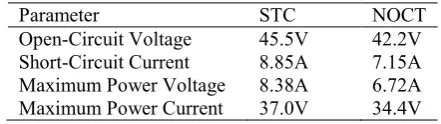
electric charge in Coulombs, k is the Boltzmann constant in m2_kgs-2_K-1 _{and T is the temperature in Kelvin. Table 1 gives}

the characteristics of the PV module used at standard testing condition (STC) [23].

Table1. Module data for Trina Solar TSM 310PD14

2.1. Calculating RS and RSH and I0

RS and RSH can be calculated using the method

proposed in [22]. I0 can be calculated using equation (2) [13].

𝐼0=

1

𝑒𝑞𝑉𝑂𝐶⁄𝑘𝑇− 1× [𝐼𝑆𝐶− 𝑉𝑂𝐶

𝑅𝑆𝐻] (2)

The Values of RS and RSH is calculated by varying their values

in equation (1) at STC and nominal operating cell temperature (NOCT). The values of RS and RSH when the calculated power

equal the module power from the PV data sheet at STC and NOCT is the module RS and RSH. The value of RS and RSH

calculated for Trina Solar TSM 310PD14 is 0.3Ω and 425Ω respectively.

2.2. Calculating ISC

The short-circuit current can be calculated for any temperature and irradiance using equation (3) [22],

𝐼𝑆𝐶,(𝐼,𝑇)=

𝑆

1000(𝐼𝑆𝐶(𝑆𝑇𝐶)+ 𝛼𝑆𝐶∗ (𝑇 − 25)) (3)

where ISC(STC) is the short-circuit current in Amperes

at STC, T is the temperature in Celsius, SC is the temperature

coefficient of the A/°C and S is the irradiance in w/m2_{. Figure}

(1) shows the graph of ISC for a wide of range of temperature

and irradiance values.

Parameter STC NOCT

3 2.3. Calculating VOC

The VOC for any combination of irradiance and

temperature can be obtained using equation (4).

𝑉

(𝑆, 𝑇) =

𝑚𝑘

∗ 298

𝑞

ln (

𝐼

(𝑆, 𝑇)

𝐼

+ 1)

+ (𝑇 − 25) ∗ 𝛼

(4)

Figure (2) gives the graph of the VOC for a wide range of

operating conditions of the PV module.

Figure 1. Module short-circuit current

Figure 2. Module open-circuit voltage

2.4. Calculating Maximum Power

The maximum power can be calculated by numerically solving equation (1). Figures (3) and (4) give the current (IMP) and voltage (VMP) at maximum power

respectively for one module of TSM310 PD14 with selected irradiance and temperature calculated using the method described in this paper.

Figure 3. Module Maximum Power Current

Figure 4. Module maximum power voltage

2.5. Operating PV at Maximum Power

The method used for operating the PV at maximum power is that presented in [14]. The calculated VMP or IMP are

the reference to the PI controller and the actual maximum power voltage or current is used as opposed to an arbitrary percentage of the VOC or ISC making the offline method much

more accurate and much more efficient. Unlike the fractional

VOC or ISC method, which will disconnect the terminals of the

module to measure the VOC, the maximum power point is

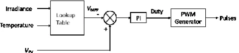
calculated offline and is therefore much more efficient. The maximum power point for all possible combinations of temperature and irradiance is stored in a look-up table which outputs the reference VMP or IMP based on

the input temperature and irradiance. The more samples of irradiance and temperature used the more accurate the approximation. Interpolation is used to estimate the maximum power point for irradiance and temperature not stored in the look-up table. Figure (5) show the MPPT operation.

Figure 5. MPPT strategy

28.8 36

1000 ₆₀

43.2

O

pe

n-C

irc

u

it

V

ol

ta

ge

(

V

)

40 50.4

Irradiance (w/m2)

20 500

Temperature (°C)

57.6

0 -20 0 -40

0 30 2 4

1000

M

ax

im

um

P

ow

er

C

ur

re

nt

(

A

)

20 6

800

Temperature (°C)

8

Irradiance (w/m2)

600 10

10

4 2.6. Creating Power Reserve

The PVPP is operated at maximum power point by obtaining the reference voltage from the look-up table. The P-V curve of the module can be used to adjust the reference voltage to create a reserve power. The voltage of PV modules is from 0-VMP as the power moves from 0-PMP and the VMP

-VOC as the power moves from PMP-0. The voltage varies

almost linearly with power from 0-PMP and varies

inverse-linearly with power PMP-0 (after PMP). A 10% reserve can be

created by using the equation either of equation (5) or (6).

𝑉

= 𝑉

× 0.9 (5)

𝑉

= (𝑉

− 𝑉

) × 0.9 + 𝑉

(6)

It is preferable to use equation (5) because the PV curve is very steep after the maximum power point. Hence, a small deviation from the desired operating point will result in a significant difference in power from power expected and

V0-VMP is more linear than VMP to VOC. This method is

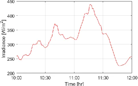
employed when a fixed percentage of maximum power is to be reserved irrespective of changes in temperature and irradiance. This reserve method has been implemented using the real irradiance in figure (6) [24]. Figure (7) shows the PVPP operating at maximum power and with a power reserve of 20%.

Another method that can be used to de-load the PVPP to create a reserve a fixed amount of power reserve (irrespective of the irradiance and temperature) is as follows. Since the VMP and IMP are known from the offline calculation,

the PMP can be easily calculated. The remaining power after

subtracting the reserve power from the maximum power to the maximum power is then calculated. The product of the ratio of the remaining power to the maximum power and VMP

becomes the reference voltage for the PI controller. Using this method, no power will be generated if the maximum available power is below the reserve power required but it guarantees a fixed amount of power reserve as long as it is available. Figure (8) shows the implementation of the fixed power de-loading method.

Figure 6. Real irradiance data [24].

Figure 7. MPPT and de-loading operation (at 25°C).

Figure 8. Fixed power de-loading.

3. Frequency Support Methods

3.1. Fast Frequency Support (FFR)

This method of support involves increasing the output power of the PVPP by a defined step in response to a change in frequency. In this method, power is released fast enough such that it affects both the ROCOF and the frequency nadir. The control is implemented by placing a switch between the MPPT look-up table and the PI controller reference voltage that switches the reference voltage between the de-loaded voltage and the maximum power voltage (or voltage corresponding to the required power increase) depending on the measured change in frequency or ROCOF. Figure (9) shows the implementation of FFR.

5

Figure 9. Fast frequency Response.

Figure 10. Droop support

Figure 11. Combined droop+inertia support

3.2. Droop Support

This method is similar to that used in conventional generators but with a faster release of active power. The response is fast enough to impact both the inertial and governor-action responses unlike the droop in conventional generators which only affects the governor-action response. This method also gives a more proportional response to a frequency events than the fast frequency method.

The frequency-voltage droop control is carried out on the reference voltage since the voltage is proportional to the power from zero volts to the maximum power voltage. The droop gain (Ddroop) determines the additional power from the

PV power plant. Figure (10) show the droop control implementation.

3.3. Inertia Emulation Support

The PVPP can also be controlled to release power emulating the inertia of synchronous generators. A similar method has been used for wind turbines in [25]. In [26], the ROCOF resulting from a generation-load unbalance is determined by equation (7),

𝐽𝜔

𝑑𝜔

𝑑𝑡

= ∆𝑃 (7)

Where m is the mechanical speed and J is the moment

of inertia. According to [26], the power delivered by extracting the kinetic energy in the rotating masses can be given as

𝑃 = 2𝐻 × 𝜔

×

𝑑𝜔

𝑑𝑡

(8)

where H is the inertia constant. The PV power can then be adjusted using equation 8 to release additional power during a frequency event and contribute to the inertial response. The measurement of the frequency change is usually filtered to remove noise [27]. As with other PV support methods, the voltage reference is adjusted to control PV power. The PV voltage is approximately proportional to the power up to maximum power due to the PV control and de-loading method used. The control for combined inertia and droop support is shown in figure (11).

3.4. Variable Droop Support

The fast-frequency response (FFR) is very effective in slowing down the ROCOF but has two major drawbacks. One is that it can over-compensate for an increase in load or loss of generation if the increase in power is not properly selected and this can cause another frequency event since the increase in power does not change as the frequency changes. The second drawback is that it gives a fixed constant output for a frequency event which will permanently reduce or completely use up the power reserve. This will reduce the ability of the PVPP to provide support in subsequent frequency events and thus making it a less reliable source of continuous frequency support.

The PV droop control, unlike the FFR, changes the output of the PVPP based on the droop slope and change in frequency, resulting in support that is proportional to the change in frequency. The PVPP droop control responds much faster than droop control in conventional generators and hence affects the frequency response in the inertia timescale. As in conventional droop control, the droop slope is constant, the speed advantage of the PVPP operating with offline MPPT is not fully exploited.

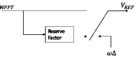
In order to take advantage of the very fast increase in power from FFR and the proportionality of the droop control. A variable droop control for the PVPP frequency support is proposed. The variable droop control can be implemented using two methods.

3.4.1 Method 1:

6 reducing the frequency nadir and slowing the ROCOF with

the proportionality of droop control. It also does leaves some reserve power immediately after the specified fast frequency support time period which can be used for providing support in subsequent frequency events.

To implement this support method, the increase in power following a frequency event has to be determined for the inertia timescale. The PV droop gain to deliver the required power increase is determined by dividing the power increase required by the change in frequency.

The function used for this paper is given by equations (9) and (10) below

𝑃

= 0.05𝑝𝑢 1 ≤ 𝑡 ≤ 4 (9)

𝑃

= 𝑃

4 < 𝑡 < 𝑡

(10)

Where Pinc is the require increased in power and t is the

simulation time. Maximum support is given till time is 4s which is within the typical timeframe for inertial response [11].

The droop gain, Dg, can be calculated using equation (11)

and (12) below.

𝐷

=

0.05𝑝𝑢

∆𝑓

𝑡

≤ 𝑡 ≤ 4 (11)

𝐷

= 𝐷

4 < 𝑡 < 𝑡

(12)

For equation (12), the droop gain returns to the set value 3s after frequency event.

3.4.2 Method 2:

For the second variable droop support method, the droop gain is gradually reduced after the inertia time scale unlike the sudden change in the droop gain used in Method 1. In this way, the reserve is slowly recovered back to the level it would be with conventional droop. This method prevents a secondary droop which can be expected when method 1 is used. This method is implemented by multiplying the droop by an equation which gives a constant increase in power during the inertia timescale and gradually decreases the power by gradually reducing the droop gain until it reaches the desired level. The droop gain after the inertia timescale is given by equation (13),

𝐷

= 𝐷

+ (𝑡 − 4) × 𝐾 4 < 𝑡 < 𝑡

(13)

7 where K is the rate at which the droop gain is reduced and tsup

is the time during which the PVPP provides support. A lower droop limit can be set so that the droop gain is not reduced indefinitely and the PVPP continues to provide support after the primary response timescale. This method also regains the power reserve that could be seen with conventional droop support but does so at a slower rate compared to that in Method 1.

4. Case Studies

4.1. Test System

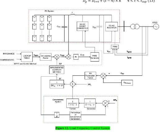
The test system consists of a grid-connected PVPP with load-frequency control as show in figure (12). The PVPP is made up of 66 parallel strings with each string having 5 series connected modules. The PV system will produce a maximum power of 100kW at STC. The conventional synchronous generation system can be represented by a single machine [28]. The equivalent system inertia is given by equation (14) [29].

𝐻

= ∑ 𝐻

𝑆

𝑆

𝑖=1

(14)

Where Ssys is the system power, Hi and Si are the inertia

constant and apparent power of each generator and n is the number of generators.

To examine the ability of the PV system to provide frequency support, the change in the PVPP output power during frequency event is measured and added to the load-frequency control system.

The different PV support methods are implemented by taking the change in frequency from the load frequency control system and adjusting the reference voltage of the PV MPPT reference voltage based on the support method employed. Figure (12) gives the load frequency control of the system.

To examine the effect of increasing penetration, the inertia of the system and the droop gain is adjusted to account for different levels of PV penetration. For example, for a 20% penetration by the PVPP, the change in power from the PVPP is multiplied by 0.2 and the change in generator power is multiplied by 0.8 while the inertia of the system reduces by 20%.

4.2. Increasing PV Penetration

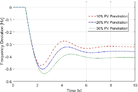
In this case, the effect of increasing the penetration of PVPP power is examined using the different support methodologies described in this paper. Figures (13), (14) and (15) show the frequency deviation for a system with 10%, 20% and 30% PV penetration for a 0.1pu load increase at t=1s. In figure (13) only the inertia support control is implemented and in figure (14), only droop control is implemented. Figure (15) shows the responses when both inertia and droop support control are implemented. Change in PV power is multiplied by 0 until 0.99s and is then multiplied by one thereafter. This is to prevent the PV from affecting the frequency deviation when as it tries to find maximum power point. The response when droop and droop+inertia is used shows that the

magnitude of the nadir is smaller and the ROCOF is slower as the PV penetration increases. This demonstrates that the PVPP adequately compensates for the reduction in inertia that comes with increasing the PV penetration. This is because the droop and droop+inertia affect the frequency deviation at the inertia timeframe more than a conventional droop. When only inertia support is used the nadir gets lower and the ROCOF higher with increasing PV penetration. The droop+inertia give the smallest nadir and slowest ROCOF as more power is provided during the inertia timeframe. The inertia control only provides support during the inertia timeframe and thus leaves a larger steady-state frequency deviation than the droop and droop+inertia. The inertia control however, leaves more reserve power after the frequency event than droop and the droop+inertia controls.

Figure (16) gives the frequency deviation using fast frequency response for 10%, 20%, and 30% penetration. The response shows that this method gives the smallest nadir and slowest ROCOF. However, this method uses up the power reserve depending on the step power increase for a given frequency event. This leaves the system with PVPP with less capacity to provide support in subsequent frequency events.

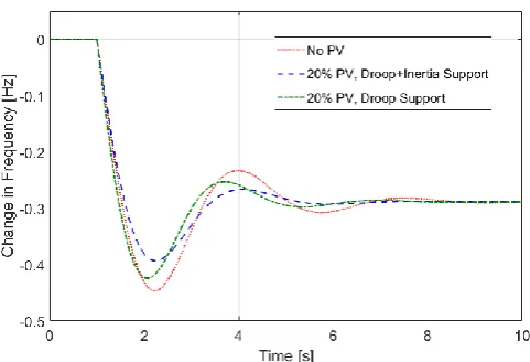
4.3. Conventional synchronous plant VS PVPP support

This case compares the frequency deviation when no PV is connected and when PV is connected with different penetration levels. Figure (17) shows the frequency deviation with no PV and with 20% PV penetration (with droop and droop+inertia support controls). Again, the load increases by 0.1pu at t=1s. The results clearly illustrate that better performance is obtained when PV is present and providing frequency support. This confirms the results from Case 1 which shows that smaller nadir and slower ROCOF are obtained as the PV penetration increases using a combined droop and inertia support control Figure (18) shows the change in power of the PVPP with and without hen it provides droop support provision. It can be seen that power from the PVPP is released much faster than the power from conventional synchronous generation. This explains the slower ROCOF and the reduced nadir observed when droop or droop+inertia are implemented in the PVPP.

8

Figure 14. Droop support (droop gain=20)

Figure 15. Droop (gain=20) + Inertia Support (K=10).

Figure 16. Fast Frequency Response.

Figure 17. Frequency response (conventional synchronous generation vs PVPP).

Figure 18. Power Change (conventional synchronous generation vs PVPP).

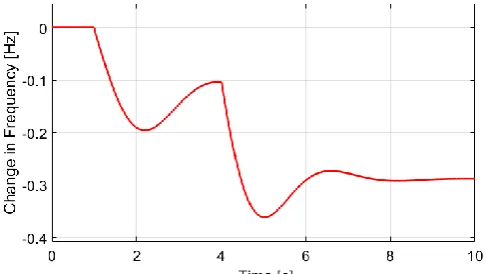
4.4. Variable Droop

9

Figure 19. Variable droop (sudden power change).

Figure 20. Change in Power (Sudden)

Figure 21. Variable droop (dradual droop).

Figure 22. Power change (gradual droop). 4.5. Effect of Available Reserve

All the support methods investigated require an increase in the PVPP power output to provide frequency support. Hence their performance and level of support they can provide is influenced by the amount of reserve power

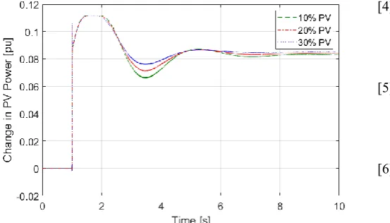
available. This case examines the effect on the frequency deviation if the available reserve is reduced to 10% of the maximum power and the PVPP uses the combined droop and inertia support control method. In figure (23), the maximum increase in the PV power output for 10%, 20% and 30% penetration levels is 16.25%, 15.27% and 14.36%, respectively (with a droop gain of 20 and inertia gain of 10 for a 0.1pu increase in load). This implies that a reserve of at least 13.98% ((16.25 ÷ 116.25) × 100), 13.25% and 12.5%, respectively will be required in order to obtain the same response.

In figure (24), the frequency deviation for 10%, 20% and 30% PVPP penetration with the reserve limited to 10% of maximum power is shown. The nadir is larger than that observed in the responses with a 20% reserve. This is because the reserve was not enough to supply the maximum power increased demanded by the combined droop and inertia support method used. This can be seen in the flat top of the change in power in figure (25) when the reserve is limited to 10%. The nadir is still smaller and the ROCOF slower for increasing penetration. Figure (23) also shows that a smaller increase in power is required to obtain the same frequency response as the PV penetration increases.

Figure 23. Change in PV power with 20% reserve

10

Figure 25. Change in power with 10% reserve.

5. Conclusions

A novel approach to enable a PVPP to provide frequency support to a power grid more efficiently has been presented. It relies on the PVPP having certain power reserve and being control using an offline MPPT technique. This technique provides better performance and speed of response in changing the operation point. Different methods to enable the PVPP to provide frequency support have been implemented and described in detail. The results show that given the proper power reserve, a PVPP can adequately compensate for the reduction in inertia caused by the increase in converter connected generation. The results also show that the proposed droop and combined droop+inertia support controls result in a slower ROCOF as the PV penetration increases. The results show that the best response is obtained by releasing as much power as possible immediately after the increase in load like with the FFR but this uses up the power reserve and reduces the ability of the system to participate in subsequent frequency events. To overcome this drawback, a variable droop method is proposed. In the proposed variable droop method, the droop gain is varied to deliver maximum available power in the first three seconds after a frequency event caused by a load increase. The droop gain is then reduced either suddenly or gradually after these 3 seconds to regain power reserve. The main disadvantage of the MPPT method used in this paper is that the calculated value of the short-circuit power or the open-circuit voltage will become less accurate over time.

6. References

[1] Suthaputchakun, C., Sun, Z., and Dianati, M.: ‘Applications of vehicular communications for reducing fuel consumption and CO2 emission: the state of the art and research challenges’, IEEE Communications Magazine, vol. 50, no. 12, pp. 108-115, December 2012.

[2] European Commission.: ‘A Framework Strategy for a Resilient Energy Union with a Forward-Looking Climate Change Policy COM(2015) 80 final’, European Commission, 2015.

[3] ‘Renewable Energy – Recast to 2030 (RED II)’,

https://ec.europa.eu/jrc/en/jec/renewable-energy-recast-2030-red-ii, accessed 15 May 2019.

[4] Morren, J., De Haan, S.W.H., Kling, W.L., and Ferreira, J.A.: ‘Wind Turbines Emulating Inertia and Supporting Primary Frequency Control’, IEEE Transactions on Power Systems, Vol. 21, NO 1, pp. 433-434, February 2006.

[5] Keung, P.-K., Li, P., Banakar, H., and Ooi, B.T.: ‘Kinetic energy of wind turbine generators for system frequency support’, IEEE Transactions on Power Systems., vol. 24, no. 1, pp. 279–287, Feb. 2009.

[6] Taheri, H., Akhrif, O., and Okou, A.F.: ‘Contribution of PV generators with energy storage to grid frequency and voltage regulation via nonlinear control techniques’, IECON 2013 - 39th Annual Conference of the IEEE Industrial Electronics Society, Vienna, 2013, pp. 42-47. [7] Attya A.: ‘Integrating battery banks to wind farms

for frequency support provision – capacity sizing support algorithm’, Journal of Renewable and Sustainable Energy, Vol 7, No 5. October, 2015 [8] Takahashi, R. and Tamura, J.: ‘Frequency control of

isolated power system with wind farm by using Flywheel Energy Storage System’, 2 008 18th International Conference on Electrical Machines,

Vilamoura, 2008, pp. 1-6.

[9] Weckx, S., D'Hulst, R., and Driesen, J.: ‘Primary and Secondary Frequency Support by a Multi-Agent Demand Control System’, in IEEE Transactions on Power Systems, vol. 30, no. 3, pp. 1394-1404, May 2015.

[10] Crăciun, B., Kerekes, T., Séra, D., and Teodorescu, R.: Frequency Support Functions in Large PV Power Plants with Active Power Reserves’, in IEEE Journal of Emerging and Selected Topics in Power Electronics, vol. 2, no. 4, pp. 849-858, Dec. 2014. [11] Rahmann; C., Castillo, A.: ‘Fast Frequency

Response Capability of Photovoltaic Power Plants: The Necessity of New Grid Requirements and Definitions’, Energies2014, 7, 6306-6322

[12] Zarina, P.P., Mishra, S. and Sekhar, P.C.: 'Exploring frequency control capability of a PV system in a hybrid PV-rotating machine-without storage system’, International Journal of Electrical Power & Energy Systems, Volume 60, 2014, Pages 258-267. [13] Hoke, A.F., Shirazi, M., Chakraborty, S., Muljadi, E. and Maksimovic, D.: ‘Rapid Active Power Control of Photovoltaic Systems for Grid Frequency Support’, in IEEE Journal of Emerging and Selected Topics in Power Electronics, vol. 5, no. 3, pp. 1154-1163, Sept. 2017.

[14] Jibji-Bukar, F., Anaya-Lara, O.: ‘Offline Photovoltaic MPPT Fyali Jibji-Bukar’, 3rd

International Conference on Power and Renewable Energy, Berlin, Sep. 2018, pp. 1-6.

[15] Mohapatra, A., Nayak, B., Das, P., Mohanty, K.B.: ‘A review on MPPT techniques of PV system under partial shading conditions’, Renewable and Sustainable Energy Reviews, vol. 80, 2017, pp. 854-867.

11 [17] Salas, V., Olías, E., Barrado, A., Lázaro, A.:

‘Review of the maximum power point tracking algorithms for stand-alone photovoltaic systems’, Solar Energy Materials and Solar Cells, Volume 90, Issue 11, 2006, Pages 1555-1578,

[18] Ishaque, K., Salam, Z.: ‘A review of maximum power point tracking techniques of PV system for uniform insolation and partial shading condition’, Renewable and Sustainable Energy Reviews, Volume 19, 2013, Pages 475-488.

[19] Ahmad, J.: ‘A fractional open circuit voltage based maximum power point tracker for photovoltaic arrays’, 2010 2nd International Conference on Software Technology and Engineering, San Juan, PR, 2010, pp. V1-247-V1-250.

[20] Elobaid, L.M., Abdelsalam, A.K. and Zakzouk, E.E.: ‘Artificial neural network-based photovoltaic maximum power point tracking techniques: a survery’, IET Renewable Power Generation, vol. 9, no. 8, pp. 1043-1063, 2015.

[21] Messalti, S., Harrag, A., and Loukriz, A.: ‘A new variable step size neural networks MPPT controller: Review, simulation and hardware implementation’, Renewable and Sustainable Energy Reviews, Volume 68, Part 1, 2017, Pages 221-233,

[22] Villalva, M.G., Gazoli, J.R. and Filho, E.R.: ‘Comprehensive Approach to Modeling and Simulation of Photovoltaic Arrays’, in IEEE Transactions on Power Electronics, vol. 24, no. 5, pp. 1198-1208, May 2009.

[23] ‘Datasheet – Trina Solar – 310W-325W – Tallmax’,

https://loopsolar.com/datasheet/trina-solar/trina-

solar-tallmax-multicrustalline-72cell-310W-325W-datasheet-india.pdf, accessed 15 May 2019.

[24] Vignola, F., Andreas, A.: ‘University of Oregon: GPS-based Precipitable Water Vapor (Data)’, NREL Report No. DA-5500-64452, 2013. http://dx.doi.org/10.7799/1183467

[25] Tielens, P., De Rijcke, S., Srivastava, K., Reza, M., Marinopoulos, A., and Driesen, J.: ‘Frequency support by wind power plants in isolated grids with varying generation mix’, 2012 IEEE Power and Energy Society General Meeting, San Diego, CA, 2012, pp. 1-8.

[26] Morren, J., Pierik, J. and de Haan, S.H.W.: ‘Inertial response of variable speed wind turbines’, Electric Power Systems Research, Volume 76, Issue 11, 2006, Pages 980-987

[27] Van de Vyver, J., De Kooning, J.D.M., Meersman, B., Vandevelde, L and Vandoorn, T.L.: ‘Droop Control as an Alternative Inertial Response Strategy for the Synthetic Inertia on Wind Turbines’, in IEEE Transactions on Power Systems, vol. 31, no. 2, pp. 1129-1138, March 2016.

[28] Kundar, P.: ‘Power System Stability and Control’, New York, US. McGraw-Hill, 1994.