Effect of the damper property variability on the seismic reliability of linear systems equipped with viscous dampers

1

Effect of the damper property variability on the seismic reliability of linear

systems equipped with viscous dampers

Andrea Dall'Asta1_{, Fabrizio Scozzese}1_{, Laura Ragni}2_{, Enrico Tubaldi}3

1_{School of Architecture and Design, University of Camerino, Viale della Rimembranza, 63100 Ascoli Piceno (AP),}

Italy; E-mail: [email protected], [email protected]

2 _{Department of Civil and Building Engineering and Architecture, Polytechnic University of Marche, Via Brecce}

Bianche Ancona (AN), Italy; E-mail: [email protected]

3 _{Imperial College London, South Kensington Campus, London SW7 2AZ, UK;}

E-mail: [email protected]

Abstract Viscous dampers are dissipation devices widely employed for seismic structural control. To date, the performance of systems equipped with viscous dampers has been extensively analysed only by employing deterministic approaches. However, these approaches neglect the response dispersion due to the uncertainties in the input as well as the variability of the system properties. Some recent works have highlighted the important role of these seismic input uncertainties in the seismic performance of linear and nonlinear viscous dampers. This study analyses the effect of the variability of damper properties on the probabilistic system response and risk. In particular, the paper aims at evaluating the impact of the tolerance allowed in devices’ quality control and production tests in terms of variation of the exceedance probabilities of the Engineering Demand Parameters (EDPs) which are most relevant for the seismic performance. A preliminary study is carried out to relate the variability of the constitutive damper characteristics to the tolerance limit allowed in tests and to evaluate the consequences on the device’s dissipation properties. In the subsequent part of the study, the sensitivity of the dynamic response is analysed by harmonic analysis. Finally, the seismic response sensitivity is studied by evaluating the influence of the allowed variability of the constitutive damper characteristics on the response hazard curves, providing the exceedance probability per year of EDPs. A set of linear elastic systems with different dynamic properties, equipped with linear and nonlinear dampers, are considered in the analyses, and Subset Simulation (SS) is employed together with the Markov Chain Monte Carlo method to achieve a confident estimate of small exceedance probabilities.

Keywords Seismic reliability; Viscous dampers; Damper properties variability; Subset simulation

1

Introduction

Supplemental energy dissipation systems are widely employed for seismic control of new and existing structures. In particular, viscous dampers have proved to be very efficient devices for dissipating the seismic input energy into heat, by reducing the displacement and inter-storey drift demand in structures (Lavan an Dargush 2009; Pavlou and Constantinou 2006). If properly designed, moment-resisting frames with added dampers could also exhibit reduced force and acceleration demands compared to conventional frames (Karavasilis and Seo 2011). To date, the performance of systems equipped with viscous dampers has been extensively analyzed by employing only deterministic approaches, neglecting the response dispersion due to the uncertainties in the input as well as in the structural system properties. However, these deterministic approaches provide only an approximate assessment of the seismic performance (Bradley 2013). Some recent works have highlighted the importance of the uncertainties in the seismic performance assessment of structures equipped with viscous dampers (Seo et al. 2014; Gidaris and Taflanidis 2015; Tubaldi et al. 2014a; Tubaldi et al 2015; Karavasilis 2016) and the different propagation of ground motion variability in systems equipped with linear or nonlinear viscous dampers (Tubaldi et al. 2014b; Tubaldi and Kougioumtzoglou 2015; Dall’Asta et al. 2016), while the work of (Lavan and Avishur 2013) has analyzed the influence of the uncertainties concerning model parameters on the seismic performance.

2

with respect to the nominal values (ASCE/SEI 2010; ASCE 41 2013; EN 15129 2010; EC8 2004), although bounded by tolerance limits allowed for the damper force. Consequently, design procedures usually involve a safety check based on the responses obtained by upper and lower bounds of the damper properties, chosen coherently with the test tolerances and modalities. However, the variability of the damper properties is generally tested in a limited range of performance levels, around some design conditions, while the reliability assessment entails evaluating a significantly wider range of performance levels. In conclusion, the actual level of safety provided by the suggested design procedures is a problem requiring further investigation, as pointed out in (Dall’Asta et al. 2016), and the relevance of this topic is mainly due to the low robustness inherent to the structure-dampers system, where the unexpected dissipative device failure can lead to a progressive collapse of the potentially non-ductile structure.

The present paper aims at evaluating the influence of these allowed tolerances in the probabilistic performance of the system, by providing information on the exceedance probability of the engineering demand parameters (EDPs) of most interest for the performance assessment (as described by response hazard curves) and by using an efficient and reliable approach.

A preliminary analysis of the damper response is firstly developed to relate the variation of the damper constitutive characteristics to the tolerance allowed in the experimental tests and to analyze the variation in the dissipation properties of the device. A second step concerns the harmonic analysis of a set of linear elastic single degree-of-freedom systems with different dynamic properties coupled with linear and nonlinear viscous dampers. The relevant sensitivity analysis permits to evaluate the effect of the parameter variations for different frequencies and amplitudes of the external input and the results can help understanding the more complex seismic response.

In the final part of the study, seismic hazard curves are developed for the set of dynamic systems considered in the previous harmonic analysis, covering different couplings between the seismic input frequency contents and the dynamic properties of the structural system. These curves provide the relation between the values of the EDPs of interest and the relevant yearly probability of exceedance. A sensitivity analysis, considering the maximum expected variation of the damper properties, is then carried out to assess the influence on the hazard curves. The EDPs considered include the maximum values of the deformation, related to the damage of the structural system and the damper failure (Pollini et al. 2016; Mijamoto et al. 2010), the maximum values of the relative velocity, related to the damper force and the maximum absolute accelerations, related to the total base reaction and the damage of acceleration sensitive devices. In order to provide amplification factors that can be compared with reliability factors suggested by the seismic codes (ASCE/SEI 2010; ASCE 41 2013), the response hazard curves are normalized by dividing the values of the EDPs by the corresponding design values.

In addition to the damper variability, the uncertainties considered in the applications concern the earthquake scenario parameters and the ground motion characteristics. Other uncertainties concerning the structural model, albeit important in some situations (Lavan and Avishur 2013, Tubaldi et al. 2011), are neglected.

It is noteworthy that the probabilistic response of the system was analyzed in many previous studies by employing approaches consistent with the PEER framework (Pinto et al. 2004; Porter 2003). This latter is a widely-employed framework that permits a separation of the tasks related to the seismic hazard, structural vulnerability and expected losses assessment. The application of the framework is usually based on a description of the seismic input in terms of a small set of real records. This approach does not permit to achieve an accurate estimate of small failure probabilities.

For this reason, in this study the Subset Simulation algorithm, with Markov Chain Monte Carlo method, is employed to obtain a good estimate of small probabilities of exceedance (Au and Beck 2001; Au and Beck 2003). This simulation techniques require a seismological stochastic model and the one proposed in (Atkinson and Silva 2000; Boore 2003) is used for the analyses.

2

Damper response sensitivity

Fluid viscous devices can either show an elastic deformation or not, depending on some minor inner manufacturing detail (i.e., presence of accumulator for preventing fluid compression). Despite a Maxwell model (i.e., an elastic spring and a viscous dashpot in series) is often employed for modelling purposes (Christopoulos and Filiatrault 2006; Symans and Constantiou 1998), in this work the compliance is neglected, and the dampers are modelled as nonlinear viscous dashpots whose constitutive law can be described in the form (Constantinou and Symans 1992; Symans and Constantiou 1998; Castellano et al. 2012)

 

v cv

 

v d

3

where v is the velocity between the damper’s end, Fd is the damper resisting force, c and  are two constitutive

parameters: the former is a multiplicative factor, while the latter describes the damper nonlinear behaviour (for the linear case).

In a sensitivity study aimed at evaluating the consequences of variations of the damper parameters on the system performance, these two parameters could be assumed to vary freely. However, the code indications on production control tests suggest a different approach to the sensitivity analysis, involving a constrained variation of the characteristic parameters directly linked to the acceptance criteria, as explained hereafter. In general, the seismic design of dissipative devices, such as viscous dampers, is based on a design value of the displacement _u* _{and velocity }*_;the

control tests are generally oriented to check the damper behavior at this design condition. In particular, sinusoidal cycles with the displacement histories _u

 

_{t u}*_sin



_v*_t/u*



_{are imposed to the damper and the corresponding maximum} damper force Fd is measured. Some tolerance is allowed in the force value and acceptance criteria usually require that the difference between the measured value of the maximum force Fd and the expected (design) value Fd* is not too

significant. More precisely, Fd must be within the interval





1p_L

 

F_d*;1p_U



F_d*



defined by the lower and upper

values (respectively pL and pU) of a tolerance parameter p (ASCE/SEI 2010; ASCE 41 2013; EN 15129 2010). The

safety check is coherently carried out by employing a lower/upper bound approach, considering the worst conditions compatible with the acceptance criteria (ASCE/SEI 2010; ASCE 41 2013; EN 15129 2010).

In this context, it is useful to establish a relationship between the variability of the response of the system equipped with the device and the outcomes of the acceptance tests. Thus, in this study the response is investigated by introducing the parameter p, describing the acceptance tolerance, and by studying the response variability for those constrained pairs of constitutive parameters

 

c,



providing the same force variation *

d

pF at the design velocity _v*_{. At this regard,}

it is useful to replace the constitutive relation of Eqn. (1) with a dimensionless one focusing on the design conditions and expressed in terms of the velocity _v* _{and the reference values of the constitutive parameters}





0 0,

c

  

_{ }



_

 

_{ *} ˆ

0

1 v

f_d   (2)

where v/v*, _/ *

d d

d F F

f  ,  cˆ/c₀, having denoted by cˆ the variation of the parameter c and by ˆ the variation of . The previous expression holds for positive velocity values only but it is sufficient for the following discussion about the constitutive parameters.

For given tolerance p, the normalized force cannot exceed the following limit value at the reference velocity

 

p

f_d1 1 (3)

and the combination of the two last equations leads to a constraint on the possible variations of c and



. This constraint associated to p can be expressed by the equation

 

 

* 1 1 ˆ

ˆ  

 _

 

v p

p (4)

where the variation cˆ_pc₀of c is not free but derives from the variation ˆ of . By substituting the expression of _p

 

ˆ according to Eqn.(2) into Eqn.(4), one obtains

_f

 

_;ˆ



_{1 p}



0ˆ

dp   (5)

As expected, f_dp

 

;ˆ is equal to 1p at the design condition (i.e., for 1), and varies by varying the velocity. In order to compare cases with different ˆ values, it is useful to observe that the ratio between the varied normalized force f_dp

 

;ˆ for a given ˆ , and for ˆ= 0, is

 

 

  

 _ˆ

0 ;

ˆ ;



dp dp

f f

4

This ratio is the same for systems with different reference pairs



c₀,₀



and it depends on the variation ˆ only. Increment or decrement of this ratio are controlled by the sign of ˆ . The ratio is equal to 1 when 1 and also for

ˆ = 0, i.e., if only c is allowed to vary (in this case, the varied forces are proportional to the reference one at all the velocities).

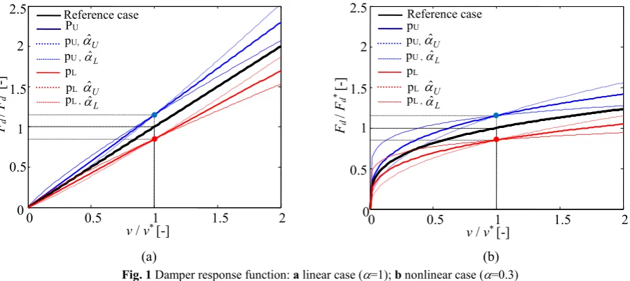
Fig. 1 describes the variation of the force-velocity relation in the neighborhood of the linear case (₀1) and the nonlinear case (₀0.3). The curves corresponding to the tolerance limit p_U 0.15 (blue curves) and p_L0.15

(red curves) are plotted and compared with the curves corresponding to the reference condition (black curves). The results concerning ˆ0 (_p  p) are reported by a red/blue solid line. The investigated range of variation of ˆ is bounded by the upper limit ˆ_U 0.137 and the lower limit ˆ_L0.152, with _pfollowing from Eqn. (4). The two

extreme -variations above (ˆ_U,ˆ_L) have been obtained by posing the normalized force ratio ˆ _{in Eqn. (6) equal to}

% 10

 at a velocity which is twice the design one (2).

It is worth to note that statistical information on the values of the variation ˆ observed in experimental tests are not available in the literature, at least to the authors’ knowledge. The investigated range of variation is such that: 1) it complies with the code’s provisions concerning the tolerance on the damper’s force response at the design velocity; 2) it is meaningful from a physical point of view, and consistent with some experimental test results (Infanti et al. 2004, Castellano et al. 2012), where the force variability can be attributed to variations of both c and  with respect to the nominal values.

It is noteworthy that according to other experimental tests (Seleemah AA, Constantinou 1997) the damper force variation may appear to be controlled by variation of c only. More experimental studies are required to investigate this aspect.

(a) (b)

Fig. 1 Damper response function: a linear case (=1); b nonlinear case (=0.3)

By referring to Fig. 1, it is possible to observe that a variation of c only (ˆ0) provides a homogeneous effect and the force variation is equal to the tolerance parameter p at all the velocity levels. More interestingly, the variation of

induces a non-homogeneous variation of the force. In the field of velocities larger than the design one (1) two curves diverge from the reference one and they correspond to the cases where ˆ has the same sign of p, i.e. pˆ0. The variations increase as the velocity increases. The remaining two cases where pˆ0provide curves approaching the reference curve when the velocity increases and intersecting it when the velocity is sufficiently large. Opposite trends can be observed for velocity levels lower than the reference one. In this case, even larger force variations can be observed for some velocity levels. The curves cannot however diverge in this case and all of them tend to zero when the velocity approaches zero.

To complete the response analysis of the device, it is useful to consider the influence of the constitutive parameters variations on the dissipative properties.

The expression of the energy dissipated in a sinusoidal cycle with circular frequency  and amplitude v/ is

0 0.5 1 1.5 2

0 0.5

1 1.5

2 2.5

Fd

/

Fd *

[-]

v / v* _[-] Reference case

pU, ˆ_U PU

pL , ˆ _L pL pU , ˆ _L

pL ˆ_U

0 0.5 1 1.5 2

0

pU, ˆ_U pU

pL , ˆ _L pL pU , ˆ _L

pL ˆ_U

Fd

/

Fd *

[-]

v / v* _[-] Reference case

[image:4.595.67.521.376.578.2]

5

 

, _1

 





cv

v

Wd (7)

where 

 

 is a geometric function related to the shape of the cycle (Symans and Constantiou 1998; Tubaldi et al. 2015). As previously, it is useful to define a dimensionless expression, w_d

 

 , obtained by dividing W_d

 

v, by the energy dissipated at the design velocity value v* by a system corresponding to the reference parameters (c0,a0) :

  

 



_{ }



 

 

     

 

0 0 0

ˆ ˆ

*

1 d

d v w

w    (8)

This ratio does not depend on the circular frequency,

 

1 0 0

d

w describes the trend observed in the reference system



c₀,₀



by varying the velocity only, and the other quantities have been previously introduced. The expression corresponding to the case of fixed tolerance p can be derived by the constraint of Eqn. (4) and the ratio between the varied and reference situation is

 

  





 

0



0 ˆ 0

ˆ 1

ˆ ;

 

    



 _ 



 p

w w

d dp

[image:5.595.66.525.456.651.2]

(9)

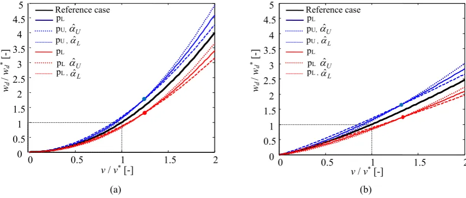
Fig. 2 describes the trend of this ratio for the upper and lower limits of p and ˆ used in the previous discussion about the force variations. Differently from the previous case, the variation ˆ influences the dissipated energy also at the reference velocity 1. As in the case of the damper forces, the curves concerning the cases with pˆ0 diverge from the reference curve for high velocity levels but in the case of the dissipated energy the intersection between the curves with different ˆ is shifted towards velocity values larger than one. The curves for the energy variation in the linear case have a parabolic trend of variation with respect to the variation of the normalized velocity while they exhibit limited variations for a variation ofˆ . In the nonlinear case, the curve curvatures are lower and the percentage variations due to a variation of ˆ are larger than the variations observed in the linear case. These different trends in the curvature and in the variation amounts provide information useful for understanding the trends in the dynamic response discussed in the following section.

(a) (b)

Fig. 2 Dissipated energy per cycle: a linear case (=1); b nonlinear case (=0.3)

3

Dynamic response sensitivity

The previous section analyzes the quasi-static response of the device under assigned sinusoidal deformation histories with different amplitude. However, the observed results cannot be directly transferred to the response of dynamical systems with nonlinear viscous dampers.

0 0.5 1 1.5 2

0 0.5

1 1.5

2 2.5

3 3.5

4 4.5

5

wd

/

wd * [

-]

v / v* _[-] Reference case

pU, ˆ_U pL

pL , ˆ _L pL pU , ˆ _L

pL ˆ_U

0 0.5 1 1.5 2

0 0.5 1 1.5 2 2.5 3 3.5 4 4.5

5 _{Reference case}

pU, ˆ_U pL

pL , ˆ _L pL pU , ˆ _L pL ˆ_U

wd

/

wd * [

-]

6

In this section, a preliminary study of the dynamic behaviour is carried out to give evidence to some qualitative results useful for understanding the seismic response discussed in the next section. For this purpose, the harmonic response of a single-degree of freedom (S-DOF) system to an input force of increasing intensity is considered. The differential equation providing the motion u

 

t is

 

t c u

 

t cu

 

t

 

u

 

t ku

 

t mA

 

t u

m  _L   sgn    sin (10)

where m is the mass, cL is the constant describing a basic linear inherent damping, c and  are the constants describing the nonlinear added viscous damper, k is the system elastic stiffness and the dots denote time derivatives.

The external input consists of a sinusoidal base motion with acceleration amplitude A and cyclic frequency . The initial conditions are assumed null, and the results shown concern the periodic stationary response observed after the transient behaviour has vanished. Reference scale values u and t can be chosen for the displacements and time respectively and the equation can be written in the dimensionless form

 

 

 

 

 



 



 

 

 



 



 _  t

u t A m

t k u

m t c m

t c_L

sin

sgn 2 2

1 2

  



  _  



 (11)

where



t/t and u/u. The problem is fully described by assigning a set of 4 dimensionless constants (Tubaldi et al. 2015; Makris and Black 2004a) and the formulation can be further simplified by relating the time scale factor to the dynamic properties of the undamped oscillator, t1/ m/k (natural period/2



). After substituting, the problem formulation reduces to

 

 

 

   

 



     

  

 _{ } 

  

    

 

   

 _{2  1 } sgn ₂ sin

u A u

m c m

c_{L    }



 (12)

The problem description is completed by assigning the other dimensionless constants:



₁c_L/m



describes the inherent damping and it is twice the usual damping factor,







2 1

2 c/m u is a term proportional to the nonlinear damping,  is the exponent describing the nonlinear behaviour, and A/2u and



/



describe the amplitude and oscillating properties of the external input respectively.

Three different dynamic systems are considered in the dynamic analysis, which differ in their characteristic periods that are: T₁0.5s (



4



), T₂1.0s (



2



), T₃3.0s (



2/3



). These values can be roughly assumed to describe the case of stiff low-rise buildings, deformable middle-rise buildings and isolated buildings, respectively. All the systems have the same inherent damping parameter



₁0.1, associated to a damping factor equal to 5%.

The analysis results obtained for the linear case (



₀1.0) and the nonlinear case (



₀0.3) are discussed and compared for three different input levels, corresponding to different normalized displacement amplitudes. The first input level corresponds to an acceleration intensity A1 selected to provide a maximum displacement demand equal to the design value uu* (max

 



 

 1), in a linear system with an additional damping described by



₂0.5, corresponding to a damping factor equal to 25%. The coefficient c0 of the reference case follows from the expression of ₂. In order to allow the comparison between the linear and the nonlinear case, the parameter



₂ of the nonlinear case and relevant c₀ are calibrated to provide the same maximum displacement of the linear case. Further information on the choice of the value u* and the calibration of the viscous coefficients can be found in Section 4.4, concerning the response to the seismic input.

The other two different levels correspond to a lower acceleration level A0.5, providing a maximum displacement equal to 0.5u, and a higher acceleration A₂, providing a maximum displacement equal to 2u. Design values reported in the following Table 1, relevant to a realistic seismic scenario, are chosen for the nonlinear harmonic analysis.

Design displacement values u* and associated acceleration amplitudes are different for the three dynamic systems but due to space constraint only the results of the system with the intermediate characteristic circular frequency



7

which is equal to the seismic design values _uu* _{of the displacements and the time scale, equal to 1/}

_

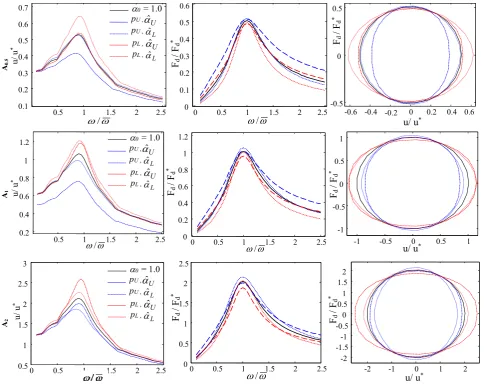
_{. This is due to} the equivalence criteria requiring similar dissipative properties for all the cases considered at _u*_{. As a consequence, the} stationary solutions and the relevant amplitudes reported hereinafter for different intensity levels and different circular frequency ratios are very similar for the three oscillators.

The results for the linear and nonlinear cases are reported respectively in Fig. 3 and Fig. 4. For each acceleration level (rows corresponding to A0.5,A1,A2), the reference solution related to the parameter pair



c0,



0



(solid black line) is compared with the varied solutions evaluated for the lower (red curves) and upper (blue curves) tolerance limits considered in the previous section (pL 0.15,pU 0.15). In both the cases, the previous two limit values of the variation of



are considered:



ˆ_L 0.152 (dashed line) and



ˆ_U 0.137 (dotted line). Reported in the figures are the maximum dimensionless displacement (first column) and the maximum damper force (second column) measured in the stable response in the circular frequency range



/







0,2.5



. In particular, the ratio between the measured damper force and the maximum value observed for the reference solution at the intermediate acceleration level, is reported. Finally, the damper force-displacement periodic response is plotted in the third column.

A0.

5

A1

A2

Fig. 3 Dynamic harmonic response for the linear reference case (₀1.0)

The maximum displacement obtained for the reference force amplitudeA₁ is analyzed first. This response parameter is influenced by the variation ˆ , as expected in consequence of the variation of the dissipative properties observed in the previous section (Fig. 2). At stable conditions the maximum displacement is controlled by the balance between the external work per cycle and the energy dissipated by the system per cycle. The variation of the external work is approximately proportional to the maximum displacement variation while the dissipated energy variation has a nonlinear dependence on the displacements, strongly influenced by the parameter



. These considerations about

-2 -1 0 1 2

-2 -1.5 -1 -0.5 0 0.5 1 1.5 2

u/ u*

0 0.5 1 1.5 2 2.5

0 0.5 1 1.5 2 2.5

0 0.5 1 1.5 2 2.5

0.5 1 1.5 2 2.5 3 u/ u *

-1 -0.5 0 0.5 1

-1 -0.5 0 0.5 1

u/ u* Fd

/ Fd

*

0 0.5 1 1.5 2 2.5

0 0.2 0.4 0.6 0.8 1 1.2  /

0.5 1 1.5 2 2.5 0.2 0.4 0.6 0.8 1 1.2  /

-0.6 -0.4 -0.2 0 0.2 0.4 0.6 -0.5

0 0.5

u/ u* Fd

/ Fd

*

0 0.5 1 1.5 2 2.5

0 0.1 0.2 0.3 0.4 0.5 0.6  / Fd / Fd

*

0.5 1 1.5 2 2.5 0.1 0.2 0.3 0.4 0.5 0.6 0.7 u/ u *

0 = 1.0

pL , ˆ _L pU ,ˆ_U pU , ˆ _L pL , ˆ_U

0 = 1.0

pL , ˆ _L pU ,ˆ_U pU , ˆ _L

pL , ˆ_U

0 = 1.0

pL , ˆ _L pU ,ˆ_U pU , ˆ _L

pL , ˆ_U Fd / F d *





/  / u/ u * Fd / F d * Fd / Fd

[image:7.595.57.542.264.651.2]

8

energy balance explain the differences observed between the linear and nonlinear cases as well as the larger variation amplitude of the latter case. For the whole range of frequencies analyzed, the maximum and minimum displacement variations are observed for the pairs pL,



ˆU and pU,



ˆL, respectively, for both the linear and nonlinear damper. As expected, the damper forces show an opposite trend; in the linear case the maximum and minimum forces are obtained for the pairs p_U,



ˆ_U and p_L,



ˆ_L, around



/



1 respectively and inverted trends, with maximum and minimum corresponding to the pairs pU,



ˆL and pL,



ˆU, are observed for



far from



.

The nonlinear response is quite different and more complex than the linear one. Unlike the linear case, larger variations can be observed around



/



1 and the response curve is generally “flatter” than the curve of the linear case. The differences measured in the damper force do not vary drastically by shifting the external force circular frequency even if, as in the case of linear damper, there are intersections causing the curves trend inversion between the resonant zone and the frequencies further from



. Thus, the cases providing the extreme force values at



/



1 are not the same providing the maximum force values for higher and lower circular frequencies. This latter feature can be of interest in the seismic analysis because it implies that an earthquake with a fixed frequency content can provide different response variations on dynamic systems with different characteristic periods.

The normalized system response changes by applying the lowest input level A_0.5 and the highest input level A₂. For A0.5, the extreme positive and negative displacements variations are still provided by the pairs pL,



ˆUandpU,



ˆL respectively (along the whole frequency range) as in the case of A1, whereas for A0.5 they are governed by the

L

p ,



ˆLandpU,



ˆU pairs around



/



1. The damper forces in correspondence of the input amplitudesA0.5and

2

A exhibit a trend opposite to that of the displacements.

All the trends qualitatively described above are consistent with the trend of variation with ˆ of the dissipated energy reported in Fig. 2, where the curves relevant to



ˆ_L and



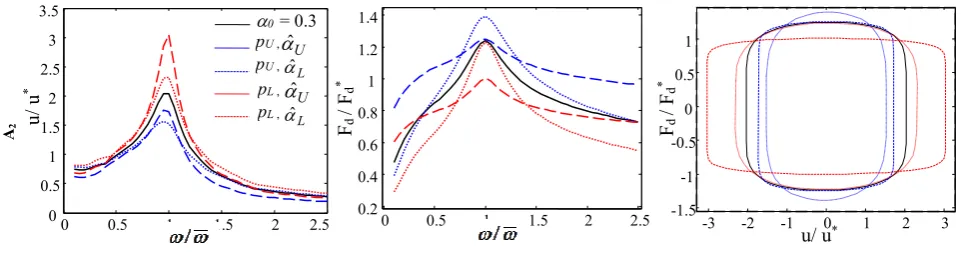
ˆU intersect at a velocity value larger than v*. The trend of the positive extreme variations of the displacements and the trend of the damper force variations can be explained on the basis of similar observations.

A0.

5

A1

-1.5 -1 -0.5 0 0.5 1 1.5 -1

-0.5 0 0.5 1

Fd / Fd

*

0 0.5 1 1.5 2 2.5 0.2

0.4 0.6 0.8 1 1.2

0 0.5 1 1.5 2 2.5

0 0.2 0.4 0.6 0.8 1 1.2 1.4

-0.8 -0.6 -0.4 -0.2 0 0.2 0.4 0.6 0.8

0 u/ u*

-0.5 0.5

0.2 0.3 0.4 0.5 0.6 0.7 0.8 0.9 1

0.5 1 1.5 2 0

Fd / Fd

*

0 0.5 1 1.5 2 2.5 0.7

0.6 0.5 0.4 0.3 0.2 0.1 0 0.8

u/

u

*

0 = 0.3

pL , ˆ _L pU ,ˆ_U pU , ˆ _L

pL , ˆ_U





/

0 = 0.3

pL , ˆ _L pU ,ˆ_U pU , ˆ _L

pL , ˆ_U

u/ u*

2.5 Fd

/ F

d

*

Fd

/ F

d

*

u/

u

9

A2

Fig. 4 Dynamic harmonic response for the nonlinear reference case (₀0.3)

4

Seismic performance sensitivity

4.1Seismic performance description

The seismic assessment and design of structures aims at ensuring that the probability that a EDP of interest D exceeds a fixed threshold d_f , P



D>d_f



, is lower than an acceptable valueP_f . The generic response D accounts for the uncertainties in the loading actions and in the system response. Typical EDPs employed in the context of performance assessment of building with viscous dampers are: inter-storey drifts, absolute floor accelerations, total base shear, damper strokes and forces.

Design codes and practical assessment procedures aim at satisfying the reliability constraint in an indirect way, by evaluating, via structural analysis, a conventional demand measure d*df for a loading level whose exceedance

probability P*is higher than the acceptable probability P_f (Bradley 2013). A series of factors is then used to increase

the demand d* up to the target value d_f (Wen et al. 2003). In the specific case of the seismic analysis of buildings equipped with dampers, the design is carried out by evaluating the response for seismic events with a mean annual frequency of occurrence approximately varying from 1·10-2 _{(serviceability limit state) to 2·10}-3 _{(ultimate limit state)}

(ASCE 7 2010; Probabilistic Model Code 2000; EC0 2002) while the safety goal is to achieve a probability of failure per year lower than 10-5_-10-6 _{(ASCE 7 2010; EC0 2002).}

In order to relate the design condition, described by the pairs



_d*_,P*



_{, to the effective failure condition, described} by the couple



df,Pf



, it is useful to evaluate first the response hazard function

 

d P



D d



GD  > (13)

associating a generic value of the EDP threshold d to the corresponding probability of exceedance. The conventional design value d* can be linked to the response value associated to a given probability of exceedance by introducing the inverse function GD-1(P) and defining the ratio

 

1

 

_*

d P G

P D

d





 (14)

This ratio can be interpreted as the amplification factor for the design value d* providing the EDP value corresponding to the desired probability of exceedance P, and _d

 

P_f can be compared with the reliability factors suggested by some recent seismic codes (ASCE 41 2013; EN 15129 2010) and used in semi-probabilistic methods for safety verifications.

Design procedures generally introduce a further simplification as they prescribe to evaluate d* by means of a deterministic analysis rather than a probabilistic one. In fact, the seismic design is usually based on the description of the seismic input in terms of a pseudo-acceleration response spectrum and a reduced set of (artificial or natural) ground motions accounting for the record-to-record variability effects. The conventional design value of the response d* is obtained as the mean of the maximum response values. This design approach introduces further sources of -3 -2 -1 0 1 2 3 -1.5

-1 -0.5 0 0.5 1

u/ u* Fd

/ Fd

*

0 0.5 1 1.5 2 2.5

0.2 0.4 0.6 0.8 1 1.2 1.4

0 0.5 1 1.5 2 2.5

0 0.5

1 1.5

2 2.5

3 3.5

u/

u

*

0 = 0.3

pL , ˆ _L pU ,ˆ_U pU , ˆ _L

pL , ˆ_U

Fd / Fd

[image:9.595.57.538.70.197.2]

10

approximation in the evaluation of the system reliability which are not addressed in this work (Bradley 2013; Wen et al. 2003).

4.2Uncertainty description

In this paper, the uncertainties taken into account concern the seismic input and the viscous damper properties, while the uncertainties in the other structural model parameters (e.g., material, geometrical properties, etc.), usually having a minor influence on the probabilistic response (Tubaldi et al. 2011), are not considered (i.e., these quantities are assumed to be deterministic). The uncertainties in the seismic input are described by a statistical model while the uncertainties in the damper properties are considered in the context of the sensitivity analysis, in order to relate the variation of these parameters to the variation of the statistical properties of the system response.In general, two different approaches can be employed for the probabilistic representation of ground motions. The first approach is a conditional intensity measure (IM)-based one, requiring the selection of a set of real ground motion records to represent the record-to-record variability effects conditional to an IM value, whereas the second one is based on a fully stochastic representation of the seismic input. This paper employs the second approach, in conjunction with Subset simulation to achieve an accurate estimate of small failure probability.

The most representative and widely used stochastic ground motion models are the Atkinson and Silva (AS) ground motion (GM) model (Atkinson and Silva 2000) and the Razeian and Der Kiureghian (RDK) GM model (2010) respectively. The former accounts for the physic process behind a seismic event (fault rupture, waves propagation trough the medium, site amplification) through an analytical description of the earthquake’s spectral distribution (the so-called source-spectrum, corresponding to the mean Fourier spectrum of the simulated accelerograms); the latter instead, consists in fitting a set of properly time-and-frequency-modulated time-signal on a suite of recorded ground motions. The two mentioned GM models differ the one to each other for many aspects, the main of which are described below. The RDK model accounts for the non-stationary spectral content, a feature of interest for structural systems whose fundamental frequencies shift during the earthquake as a consequence of hysteretic behaviour. Being the model parameters calibrated on a specific seismic database the use is constrained within a limited range of seismic scenarios. The record-to-record variability is also well-accounted for. The AS model does not account for the spectral variability and the record-to-record variability needs to be improved by adding some external source of variability (Jalayer and Beck 2008). However, this model can be used in a wide range of seismic scenarios. The presented study concerns structural systems with fixed resonant frequency and the AS GM model has been preferred due to its greater flexibility.

The seismic input is described by defining a seismic source characterized in terms of moment magnitude M and source-to-site (hypo-central) distance R. This description is completed by the specification of a stochastic ground motion model accounting for the properties of the construction site. The intensity of the seismic event is described by the moment magnitude M and its uncertainty is modeled by the Gutenberg-Richter law defined in the interval [mmin,

mMAX] and corresponding to the following PDF of M given an earthquake event (Gutenberg and Richter 1958):

 

MAX e e

e p_M m _m m _m

 



 



 

min m



mmin,mMAX



 (15)

where = ln(10)b (through the parameter b) is a parameter related to the number of the expected earthquakes per year with magnitude exceeding m. More precisely, it is assumed that the occurrence of an event with M > m is a Poisson process with exceedance frequency (m) = 10a-bmand no event is expected for M > mMAX. It is also assumed that no

significant response is observed for M < mmin, so the response hazard function, referred to a time interval one year long,

can be obtained as _G

 

_d



1 _e Mmmin



_P



_D>_d|_M>_mmin



d    by starting from the outcomes of the subset

procedureP



D>d|M >m_min



.

The ground motion is generated by starting from a white noise w(t), described by the N-dimensional vector w of values

w

_i assumed at the instant ti = it, where t is the finite time interval assumed for the numerical integration.

11

frequency f while _modis a scaling factor describing the amplitude variability (Jalayer and Beck 2008). The final ground motion acceleration a(t) is obtained by the inverse Fourier transform of z

 

f _modS

 

f . The time modulating function and the radiation spectra S depend on the moment magnitude, the distance and the local characteristic of soil. The scaling factors _mod are generated from a random variable with lognormal distribution and unit median value. Further details on the ground motion model are reported in Appendix 1.

The set of variables



m,r,_mod,w



describes the motion and consists of the three scalar quantities m, r, and the vector-valued quantity w whose dimension N depends on the discretization of the time interval.

4.3Response hazard curve evaluation

Let X be the vector valued random variable of the system lying in the domain , including both the variables describing the ground motion, for which a stochastic model is required, and the structural system uncertainties. The system parameters are described by the vector  collecting the damper parameters p and ˆ , as discussed in the previous section.

The performance measure is a random variable D, whose values are positive, d0. The exceedance of a generic value d of the EDP, corresponds to the sub-region _d

 

 



x:g_D



x|



>d



, having denoted with

 

_{R}

g_D x| : the response function providing the value of the parameter

d

, once the samples

x

and the parameters  are assigned. The response hazard function can be computed as



d



I



x

  

p xdx

G_D |



_d | _X



 (16)

where p_X

 

x if the probability density function (PDF) of the system variables and I_d



x|



is an indicator function, such that I_d 1 if x_d

 

 (equivalently g_D



x|



d), otherwise I_d 0. In the following, it is assumed that

 

x X

p is not influenced by , although the formulation can be extended to the general case p_X



x|



(Au 2015). According to the prescriptions of the Annex C of the European seismic code (EC0 2002) concerning the required structural performance, for systems belonging to intermediate reliability classes (RC2 in EC0), a failure probability of the order of magnitude of 10-6 _{has to be considered (reliability index =4.75 of EC0) for the ultimate limit state}

condition to ensure a proper structural safety level. For this reason, the probabilistic analyses carried out in this paper are oriented to estimate the response hazard curves up to the probability of exceedance GD=10-6.

The solution of the reliability problem expressed by the integral of Eqn. (16) requires resorting to simulation. However, given the very small probabilities involved in this problem, it is not possible to use the robust direct Monte Carlo (MC) approach, because too many samples and simulations would be required to achieve confidence in the failure probability estimates (e.g. at least 106 _{million samples would be required to ensure a coefficient of variation of 10% in}

the estimates of a failure probability of the order of 10-4_{). For this reason, the Subset Simulation (SS) method (Au and}

Beck 2001; Au and Beck 2003) with Markov chains Monte Carlo (MCMC) method is adopted in this work. The idea behind the SS method is that the failure domain f can be decomposed into a nested sequence of domains corresponding to progressively "less-rare" events f mm1...1 in such a way that the target small probability P

 

_f P

 

_m can be viewed as a product of larger (conditional) probabilities

 

1





1 1 1

( _m) m_{i i} | _i

P P  



_ P _  . The intermediate probabilities can be conveniently estimated via the Markov chain Monte Carlo method, which allows to generate samples with a conditional probability distribution p(x|i).

A synthetic description of the method is given below. Fist, a direct MC analysis is performed in order to preliminarily investigate the domain . N independent identically distributed (i.i.d.) samples are generated, each one of whom furnishes a corresponding response value gD. Once a fixed percentile ps(a convenient value suggested in Au

and Beck 2001, also used in this work, is represented by ps=10%) has been chosen, it is possible to adaptively estimate

a response threshold d1 as the percentile value P



gD



x|



>d1



ps; by this way, a first intermediate failure region







1



1 x:gD x| >d

 is identified and, despite it is quite far from the target one m it contains useful information

12

generating new N(1-ps) conditional samples able to further populate the region ₁. This is possible thanks to the

Modified Metropolis algorithm that, starting from each seed distributed as p_X

 

x , generate new conditional samples (i.e., distributed as pX



xx1



) as states of a Markov chain (a process in which the next state depends on the current one only). According to the Metropolis algorithm the current value of a chain’s state is used for the generation of the next one by means of a properly chosen proposal pdf having the role of furnishing a next-state candidate; this last can be accepted as next state or rejected based on the fulfilment of an accept-reject rule. A discussion about the possible choice of the proposal pdf can be found in Au and Beck (2001). Once N samples are available in ₁, a new threshold level d2 is adaptively identified as the 10% percentile of the new N samples lying in ₁and the MCMC procedure is

repeated until the target failure probability P(_m) has been estimated.

It is noteworthy that although the intermediate failure probabilities are introduced for computational reasons, they can be used to effectively estimate the full response hazard curve as they provide the values of the demand corresponding to exceedance probabilities higher than the failure probability (Au and Beck 2001; Au and Beck 2003).

4.4Results

In order to evaluate different coupling between the dynamic system properties and the seismic input frequency content, the three S-DoF systems with different characteristic periods, previously introduced, are considered to study the seismic response. As previously, two added dissipative systems are analysed, the former is a linear one with ₀ 1.0 and the latter is a nonlinear one with ₀ 0.3.

The viscous constant c for the linear system has been designed to add a damping factor equal to 0.25, whereas the one for the nonlinear system has been calibrated to provide similar performances at the design conditions. More precisely, the equivalence has been established by considering the value u* assumed by the displacement hazard curve

 

_u*

G_U for P = P* _{as performance indicator. For each of the three characteristic periods considered, the linear and}

nonlinear damping system provide the same values of u* at the probability of exceedance P*GU(u*)=0.0021 (10% within 50 years); this probability value is usually assumed to define the seismic design loading for ultimate limit state conditions (ASCE 7 2010; Probabilistic Model Code 2000; EC0 2002).

The dynamic response is controlled by (11), modified as follows (Tubaldi et al. 2015)

 

 



 



   



 

  

 

 

   

    _{2 1}  sgn   

u m

c m

c_L

(17)

where the dimensionless time history 

 

 is the ratio between the base acceleration time history and the reference acceleration value u2.

The seismic scenario is defined by the following values of the seismic hazard parameters: a4.5, b1.0, mmin = 5,

mMAX = 8. The time histories are generated coherently with the Atkinson-Silva model, synthetically reported in the

Appendix, by assuming a fixed hypo-central distance r20km , and the soil conditions are described by s

m

V_S 310 / (corresponding to stiff soil, Boore and Joyner 1997).

[image:13.595.65.535.88.210.2]

13

Table 1 Properties of the damping systems and relevant response at the design conditions

Characteristic period  s 0.5 1.0 3.0

Viscous Properties



₀  1.00 0.30 1.00 0.30 1.00 0.30

m

c₀/ [s_/m_{] 6.283 2.486 3.142 1.360 1.047 0.364}

Demand at _P* _u* _{[m] 0.026 0.026 0.060 0.060 0.132 0.132}

*

v [m/s] 0.34 0.32 0.45 0.43 0.49 0.51

*

d

F [N] 432.11 350.21 284.12 210.50 102.73 59.31

*

a [m/s2_{] 4.59 4.44 2.65 2.62 0.78 0.73}

Subset simulation is performed to estimate the reliability of the damped systems for both the linear and nonlinear viscous dampers cases. A time-intervalt0.02s is considered, corresponding to N=3750. In order to estimate exceedance probabilities up to 10-6_{, the simulations are carried out using 6 conditional levels (with threshold levels}

identified by a percentile equal to 10%) with 1500 samples/level and a total number of samples equal to 1350x5 + 1500 = 8250. The result shown hereafter are the average of 50 independent simulations.

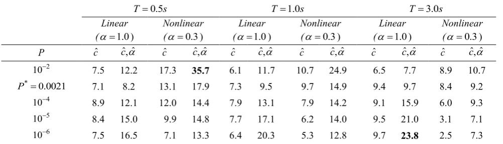
The first part of the following discussion compares the response hazard curves of the reference systems obtained by considering the nominal damper properties. These curves are expressed by the ratio d(see Eqn. (14)), providing the

values of amplification or reliability factors accounting for the effects of the variability of the seismic input only. The second part analyses the effects of the variability of the viscous damper properties, showing the variation of the factors

d with respect to the reference condition. The approach followed is consistent with the suggestion given by the

European code of practice on anti-seismic devices (EN 15129 2010), where the damper force amplification factor to be used in the safety check is split into two contributions accounting separately for these two different sources of uncertainties. On the other hand, no clear indications are furnished on the displacement amplification for the stroke safety check.

4.5Probabilistic response at the reference conditions

At the reference conditions (p0 ,ˆ0), the set of uncertain parameters considered for the performance assessment consists of those characterizing the earthquake excitation, i.e., the magnitude m, the white-noise components

w

_i, for I = 1, 2, ..., N, and the model error_mod. As already discussed, the structural system parameters are assumed to be deterministic.

Fig. 5 reports and compares the hazard curves of the systems with different characteristic periods obtained by considering the linear and nonlinear added dampers. Because of the adopted design criterion, the linearly and nonlinearly-damped systems with the same vibration period are also characterized by the same displacement u* at the probability of exceedance _P*_{while the other EDPs exhibit different values. The ratios }

d (see Eqn. (14)) between the

demand parameters and the reference values corresponding to the design conditions are reported in the horizontal axes of Fig. 5.

The linearly- and nonlinearly-damped systems exhibit different probabilistic responses within the considered range of exceedance probabilities up to 10-6_{. Since the displacement and velocity hazard curves have very similar trends, only}

the curves for the former EDP are shown in the figures. As expected, the linear and nonlinear curves intersect at P*and the relevant displacement ratioU is equal to 1.0. For probabilities of exceedance lower than P*, the displacement ratios _U observed in the nonlinear case are larger than the corresponding ones observed in the linear case, confirming that the nonlinear solution becomes more demanding than the linear one for rare events. An opposite trend is observed for probabilities of exceedance larger than the design one.

14

required by the nonlinear system is generally higher than that required by the linear system both for frequent (_PP*₎ and rare (_PP*_{) events.}

Similar qualitative trends can be observed in all the three cases corresponding to different periods of vibration but the quantitative results are different. In fact, for a given target probability level, larger values of the ratios d are

obtained for the displacements and velocities by increasing the characteristic periods, while smaller differences are observed for the absolute accelerations

.

The observed trends are consistent with those reported in previous studies carried out on similar dynamic systems (Tubaldi et al. 2014) and obtained by employing a conditional IM-based approach.

T Displacements Damper forces Absolute accelerations

0.5s

1.0s

3.0s

Fig.5 Normalized response hazard curves for linear (=1.0) and nonlinear (= 0.3) dampers

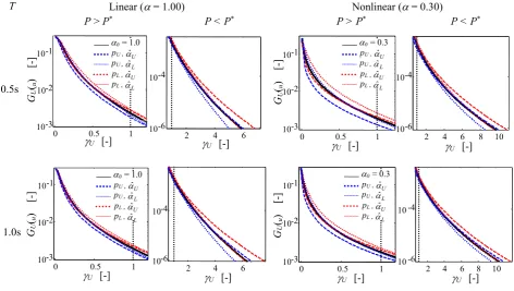
4.6Effect of viscous damper properties variability

This section illustrates and discusses the influence of the variability of the viscous damper properties on the response hazard curves. In Figs. 6-9, the response hazard curves of the previous section obtained for the set of linear and nonlinear cases by considering the reference damper parameters are presented together with the corresponding curves obtained for the varied damper parameters. As for the previous analyses concerning the damper constitutive response and the system dynamic response, the two limit values pL = - 0.15 and pU = + 0.15 are assumed for the variation of the

force at the design conditions and the extreme values



ˆ_L0.152 and



ˆU = + 0.137 are considered for the variation of the exponential coefficient. In the horizontal axis of the plots, the EDPs are normalized by their corresponding reference values (i.e., those related to the probability P*_{). When necessary to improve readability, the results observed}

10-2 100

10-6

10-4

10-2

U [-]

 = 1.0

 = 0.3

GU (u

)

[-]

10-2 100

10-6

10-4

10-2

U [-]

 = 1.0

 = 0.3

GU (u

)

[

-]

100 102

10-4

10-2

U [-]

 = 1.0

 = 0.3

GU (u

)

[-]

100 101

10-6

10-4

10-2

 = 1.0

 = 0.3

GFd (Fd

)

[-]

Fd [-]

100 101

10-6

10-4

10-2

Acc [-]

 = 1.0

 = 0.3

GA

(a

)

[-]

100 101

10-6

10-4

10-2

 = 1.0

 = 0.3

GFd (Fd

)

[-]

Fd [-]

100 101

10-6

10-4

10-2

Fd [-]

 = 1.0

 = 0.3

GFd (Fd

)

[-]

100 101

10-6

10-4

10-2

Acc [-]

 = 1.0

 = 0.3

GA

(a

)

[-]

100 101

10-6

10-4

10-2

Acc [-]

 = 1.0

 = 0.3

GA

(a

)

[image:14.595.59.526.197.580.2]

15

for values of d < 1 (with a probability of exceedance P > P*) are shown separately from the results observed for d > 1

[image:15.595.56.529.437.704.2]

(relevant to probability of exceedance P < P*_).

Fig. 6 reports the displacement hazard curves for both the linear and the nonlinear case corresponding to different variations of c and . Consistently with the harmonic analysis results (see Figs. 3-4, case A2), in the field of rare events

(_PP*_{), the largest differences are measured for the variation pair}

L L

p ,ˆ (most demanding case) and p_U,ˆ_U (least demanding case). In the field of frequent events (_PP*_{), the most demanding case corresponds to the pair}

U L

p ,ˆ and the least demanding to the pair p_U,ˆ_L. These results are consistent with those of harmonic analysis (Figs. 3-4, case A0.5)

as well.

The trends of the curves of the velocity _V , reported in Fig. 7, are similar to the trends of the displacements, and the parameters pairs furnishing the extreme variations in the fields of frequent and rare events are the same of those of the displacement curves, as expected. In Fig. 8, the damper force hazard curves are reported. These response parameters are derived quantities obtained from velocities via a nonlinear constitutive law. Since the constitutive parameters vary on a case-by-case basis, the trends of variation for the force hazard curves are significantly different from those for the velocity curves. In particular, the observed variations are higher than velocity variations also in the neighborhood of the linear case, as a consequence of the combined variations of the velocity and of the constitutive parameters. Moreover, differently from the previous case of kinematic quantities and consistently with the harmonic analysis results, the extreme variations in the field _PP* _{is obtained for the pairs}

U U

p ,ˆ (most demanding case) and p_L,ˆ_L (less demanding case). Differently, for _PP*_{, the most demanding case is obtained with the pair}

L U

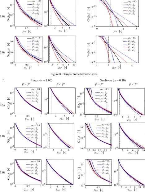
p ,ˆ and the less demanding one with the pair pL,ˆU. Fig. 9 shows the hazard curves of the absolute acceleration. The probability of

exceedance of the absolute accelerations is less sensitive to the variations of the damper properties. This quantity is proportional to the total force acting on the system, and thus it is affected by both the damper forces and the elastic system forces, proportional to the displacements, showing opposite sensitivity with respect to the parameter variations.

In the field _PP*_{, positive extreme variations occur for}

L L

p ,ˆ and extreme negative variations for p_U,ˆ_U. Some notable variations are observed in the field of very frequent events with _P102_{, in the nonlinear case.}

T Linear ( = 1.00) Nonlinear ( = 0.30)

0.5s

P > P* _{P < P}* _{P > P}* _{P < P}*

1.0s

2 4 6 8 10 -6

-4

U [-]

0 0.5 1

10 -3 10 -2 10 -1

GU (u

)

[-]

U [-]

0 = 0.3

pU, ˆ_L pL , ˆ_U pL , ˆ_L pU , ˆ_U

2 4 6

10 -6 10 -4

U [-]

0 0.5 1

10 -3 10 -2 10 -1

U [-]

0 = 1.0

pU, ˆ_L pL , ˆ_U

pL , ˆ_L pU , ˆ_U

GU (u

)

[-]

]

2 4 6 8 10 -6

-4

U [-]

0 0.5 1

10 -3 10 -2 10 -1

GU (u

)

[-]

U [-]

0 = 0.3

pU, ˆ_L pL , ˆ_U pL, ˆ_L pU , ˆ_U

2 4 6

-6 -4

U [-]

0 0.5 1

10 -3 10 -2 10 -1

U [-]

GU (u

)

[-]

0 = 1.0

pU, ˆ_L pL , ˆ_U pL , ˆ_L pU , ˆ_U

10 10

10 10

10