preconditioning for the high order edge finite elements
applied to the time-harmonic Maxwell’s equations
Marcella Bonazzoli1, Victorita Dolean1,2, Fr´ed´eric Hecht3, and Francesca Rapetti1
1Universit´e Cˆote d’Azur, CNRS, LJAD, France. E-mail: [email protected], [email protected], [email protected]
2University of Strathclyde, Glasgow, UK. E-mail: [email protected] 3
UPMC Univ Paris 6, LJLL, Paris, France. E-mail: [email protected]
Abstract
In this paper we focus on high order finite element approximations of the electric field combined with suitable preconditioners, to solve the time-harmonic Maxwell’s equations in waveguide configurations. The implementation of high order curl-conforming finite elements is quite delicate, especially in the three-dimensional case. Here, we explicitly describe an implementation strategy, which has been embedded in the open source finite element software FreeFem++ (http://www.freefem.org/ff++/). In particular, we use the inverse of a generalized Vandermonde matrix to build basis functions in duality with the degrees of freedom, resulting in an easy-to-use but powerful interpolation operator. We carefully address the problem of applying the same Vandermonde matrix to possibly differently oriented tetrahedra of the mesh over the computational domain. We inves-tigate the preconditioning for Maxwell’s equations in the time-harmonic regime, which is an underdeveloped issue in the literature, particularly for high order discretizations. In the numerical experiments, we study the effect of varying several parameters on the spectrum of the matrix preconditioned with overlapping Schwarz methods, both for 2d and 3d waveguide configurations.
Keywords: High order finite elements; edge elements; Schwarz preconditioners; time-harmonic Maxwell’s equations; FreeFem++.
1
Introduction
Developing high-speed microwave field measurement systems for wireless, medical or engi-neering industries is a challenging task. These systems often rely on high frequency (from 1 to 60 GHz) electromagnetic wave propagation in waveguides, and the underlying math-ematical model is given by Maxwell’s equations. High order finite element (FE) methods make it possible, for a given precision, to reduce significantly the number of unknowns, and they are particularly well suited to discretize wave propagation problems since they can provide a solution with very low dispersion and dissipation errors. However, the resulting algebraic linear systems can be ill conditioned, so that preconditioning becomes mandatory when using iterative solvers.
An appropriate choice to describe the electric field solution of a waveguide propagation problem is a discretization by edge Whitney finite elements [1, 2]. Here we consider the high order version of these FEs developed in [3, 4] (for other possible high order FE bases see for example [5, 6, 7, 8, 9]). We added high order edge FEs to the open source software FreeFem++ [10]. FreeFem++ is a domain specific language (DSL) specialized in solving boundary value problems by using variational methods, and it is based on a natural tran-scription of the weak formulation of the considered boundary value problem. The user can add new finite elements to FreeFem++ by defining two main ingredients: the basis functions
and an interpolation operator. The basis functions in FreeFem++ are constructed locally, i.e. in each simplex (triangle or tetrahedron), without the need of a transformation from the reference simplex; the chosen definition of high order basis functions fits perfectly this local construction feature since it involves only the barycentric coordinates of the simplex. For the definition of the interpolation operator, in the high order case we need a general-ized Vandermonde matrix, introduced for example in [11], to have basis functions in duality with the chosen degrees of freedom. In the case of barycentric coordinates the generalized Vandermonde matrix is independent of the simplex, up to a renumbering of its vertices that we carefully address here. A construction of high order edge finite elements using Cartesian coordinates can be found in [12].
For Maxwell’s equations in the time domain, for which an implicit time discretization yields at each step a positive definite problem, there are many good solvers and precondi-tioners in the literature: multigrid or auxiliary space methods, see e.g. [13] for low order finite elements and [14] for high order ones, and Schwarz domain decomposition methods, see e.g. [15]. In this paper, we are interested in solving Maxwell’s equations in thefrequency domain, also called thetime-harmonic Maxwell’s equations: these involve the inherent dif-ficulties of theindefinite Helmholtz equation, which is difficult to solve for high frequencies with classical iterative methods [16]. It is widely recognized that domain decomposition methods or preconditioners are key in solving efficiently Maxwell’s equations in the time-harmonic regime. The first domain decomposition method for the time-time-harmonic Maxwell’s equations was proposed by Despr´es in [17]. Over the last decade, optimized Schwarz methods were developed, see for example [18, 19, 20] and the references therein.
The development of Schwarz algorithms and preconditioners for high order discretiza-tions is still an open issue. A recent work for the non overlapping case is reported in [21]. In the present work, we use overlapping Schwarz preconditioners based on impedance transmis-sion conditions for high order discretizations of the curl-curl formulation of time-harmonic Maxwell’s equations. Note that domain decomposition preconditioners are suited by con-struction to parallel computing, which is necessary for large scale simulations. The coupling of high order edge finite elements with domain decomposition preconditioners studied in this paper has been applied in [22] to a large scale problem, coming from a practical application in microwave brain imaging: there, it is shown that the high order approximation of degree 2 makes it possible to attain a given accuracy with much fewer unknowns and much less computing time than the lowest order approximation.
The paper is organized as follows. In Section 2 we introduce the waveguide time-harmonic problem and its variational formulation. In Section 3 we recall the definition of basis func-tions and degrees of freedom that we adopted here as high order edge FEs. Then, in Section 4 we describe in detail the implementation issues of these FEs, the strategy developed to over-come those difficulties and the ingredients to add them as a new FE in FreeFem++. The overlapping Schwarz preconditioners we used are described in Section 5, followed in Section 6 by the numerical experiments, both in two and three dimensions.
2
The waveguide problem
Waveguides are used to transfer electromagnetic power efficiently from one point in space, where an antenna is located, to another, where electronic components treat the in/out in-formation. Rectangular waveguides, which are considered here, are often used to trans-fer large amounts of microwave power at frequencies greater than 2 GHz. In this sec-tion, we describe in detail the derivation of the simple but physically meaningful bound-ary value problem which simulates the electromagnetic wave propagation in such waveg-uide structures. To work in the frequency domain, we restrict the analysis to a time-harmonic electromagnetic field varying with an angular frequency ω > 0. For all times t ∈ R, we consider the representation of the electric field E and the magnetic field H as
E(x, t) =<(E(x)eiωt),H(x, t) =<(H(x)eiωt),where E(x), H(x) are the complex
c
x z y
b
a
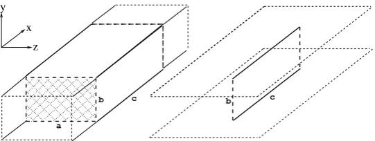
[image:3.595.163.434.83.185.2]b c
Figure 1: Rectangular waveguide configuration for 3d (left) and 2d (right) problems with wave propagation in the x-direction. The physical domain D is in thin line, with dashed style for those boundaries that should be extended to infinity. The computational domain Ω is in thick line, with dashed style for those boundaries where suitable absorbing conditions are imposed.
model is thus given by the (first order)time-harmonic Maxwell’s equations:
∇ ×H=iωεσE, ∇ ×E=−iωµH,
where µ is the magnetic permeability and εσ the electric permittivity of the considered
medium inD. To include dissipative effects, we work with a complex valuedεσ, related to
the dissipation-free electric permittivityεand the electrical conductivity σby the relation εσ =ε−iσω. This assumption holds in the regions ofD where the current densityJ is of
conductive type, that is, J and E are related by Ohm’s law J = σE. Both ε and µ are assumed to be positive, bounded functions. Expressing Maxwell’s equations in terms of the electric field, and supposing that µ is constant, we obtain the second order (or curl-curl) formulation
∇ ×(∇ ×E)−γ2E=0, (1)
where the (complex-valued) coefficientγ=ω√µεσ, withεσ=ε−iσ/ω. Note that ifσ= 0,
we haveγ= ˜ω, ˜ω=ω√µεbeing the wavenumber.
Equation (1) is to be solved in a suitable bounded section Ω of the physical domainD, as shown in Fig. 1. In the 3d case, the physical domainD ⊂R3is an infinite ‘parallelepiped’
parallel to the x-direction and the computational domain is a bounded section, say Ω = (0,X)×(0,Y)×(0,Z) = (0,c)×(0,b)×(0,a) of D. In the 2d case, the physical domain
D ⊂R3is the space contained between two infinite parallel metallic plates, sayy= 0,y=b,
and all physical parametersµ, σ, ε have to be assumed invariant in the z-direction. The computational domain in 2d is a bounded section, say Ω = (0,X)×(0,Y) = (0,c)×(0,b), of
D. In both 2d and 3d cases, the wave propagates in thex-direction within the domain. Let nbe the unit outward normal to∂Ω. We solve the boundary value problem given by equation (1), with metallic boundary conditions
E×n=0, on Γw, (2)
on the waveguide perfectly conducting walls Γw = {x ∈ ∂Ω, n(x)·ex = 0}, with ex =
(1,0,0)t, and impedance boundary conditions
(∇ ×E)×n+iηn×(E×n) =gin, on Γin, η∈R+,
(∇ ×E)×n+iηn×(E×n) =gout, on Γout,
(3)
at the waveguide entrance Γin={x∈∂Ω, n(x)·ex<0}, and exit Γout ={x∈∂Ω, n(x)·
ex>0}. The vectors gin, gout depend on the incident wave. On one hand, the impedance
conditions on the artificial boundaries Γin, Γout are absorbing boundary conditions, first
The variational (or weak) formulation of problem (1) with boundary conditions (2) and (3) is: findE∈V such that
Z
Ω
h
(∇ ×E)·(∇ ×v)−γ2E·vi+
Z
Γin∪Γout
iη(E×n)·(v×n)
=
Z
Γin
gin·v+
Z
Γout
gout·v ∀v∈V, (4)
with V = {v ∈ H(curl,Ω),v×n = 0 on Γw}, where H(curl,Ω) is the space of square
integrable functions whose curl is also square integrable. For a detailed discussion about existence and uniqueness of solutions we refer to [23]. Note that in this paper we chose the sign convention with e+iωt in the time-harmonic assumption, and therefore negative
imaginary part in the complex valued electric permittivity εσ = ε−iσ/ω and positive
parameterη in the impedance boundary condition (3).
3
High order edge finite elements
Consider a simplicial (triangular in 2d, tetrahedral in 3d) meshTh over ¯Ω, wherehdenotes the maximal diameter of simplices inTh. The unknown Eand the functional operators on it have meaningful discrete equivalents if we work in the curl-conforming finite dimensional subspace Vh ⊂H(curl,Ω) of N´ed´elec edge finite elements [24]. High order curl-conforming
finite elements have become established techniques in computational electromagnetism. We adopt the high order generators of N´ed´elec elements presented in [3, 4]: the definition of these generators is rather simple since it only involves the barycentric coordinates of the simplex T ∈ Th (see also [8] for previous work in this direction). Denote by λni the barycentric coordinate of points inT with respect to the node ni ofT.
To state the definitions and further properties, we need to introduce multi-index nota-tions. A multi-index is an arrayk = (k1, . . . , kν) of ν integers ki ≥0, and its weight k is Pν
i=1ki. The set of multi-indicesk withν components and of weightk is denotedI(ν, k).
If d= 2,3 is the ambient space dimension, we consider ν ≤d+ 1 and, given k∈ I(ν, k), we setλk =Qν
i=1(λni)
ki, where then
i areν nodes of the d+ 1 nodes of T. Now, in the
generators definition we takeν =d+ 1 andk=r−1, withrthe polynomial degree of the generators. Denote byE(T) the set of edges ofT.
Definition 3.1(Generators). Theλkwe, withk∈ I(d+ 1, k),k=r−1 ande∈ E(T), are
the generators for N´ed´elec edge element spacesW1
h,r(T) ofdegree r≥1 in a simplexT ∈ Th.
Thewe are the low order edge basis functions, namely we= λ
ni∇λnj −λnj∇λni for the oriented edgee={ni, nj}.
In Section 1.2 of [24] W1
h,r(T)-unisolvent dofs are presented, for any r ≥ 1 (the space
W1
h,r(T) is indeed a discrete counterpart of H(curl, T) ={v ∈L2(T)3,∇ ×v∈ L2(T)3}).
By relying on the generators introduced in Definition 3.1, the functionals in [24] can be recast in a new more friendly form as follows (see details in [11], which are inspired by [23]).
Definition 3.2 (Degrees of freedom). Forr≥1,d= 3, the functionals
ξe:w7→
1
|e| Z
e
(w·te)q, ∀q∈Pr−1(e), ∀e∈ E(T), (5)
ξf:w7→
1
|f| Z
f
(w·tf,i)q, ∀q∈Pr−2(f), ∀f ∈ F(T), (6)
tf,itwo independent sides off, i= 1,2,
ξT:w7→
1
|T| Z
T
(w·tT ,i)q, ∀q∈Pr−3(T), (7)
4
1
e2 e
3
e
4
e
6
e
5
1
2
[image:5.595.249.347.83.176.2]3 e
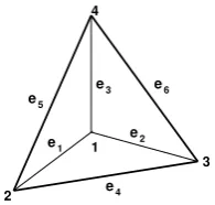
Figure 2: For the tetrahedron in the figure, the edges aree1={1,2},e2={1,3},e3={1,4}, e4={2,3},e5={2,4},e6={3,4}, the faces aref1={2,3,4},f2={1,3,4},f3={1,2,4}, f4={1,2,3}(note that the face fi is the one opposite the node i).
are the dofs for a functionw∈Wh,r1 (T), withF(T) the set of faces ofT. The norm of the tangent vectorste,tf,i,tT ,iis the length of the associated edge. We say thate, f, T are the
supports of the dofsξe, ξf, ξT.
Note that for d = 2, the dofs are given only by (5) and (6) substituting f with the triangle T; similarly, in the following, when d = 2, what concerns volumes should not be taken into account and what concerns facesf actually concerns the triangleT.
Remark 3.3. To make the computation of dofs easier, aconvenient choice for the polynomials qspanning the polynomial spaces over (sub)simplicese, f, T that appear in Definition 3.2 is given by suitable products of the barycentric coordinates associated with the nodes of the considered (sub)simplex. The spacePρ(S) of polynomials of degree≤ρover ap-simplexS
(i.e. a simplex of dimension 1≤p≤d) can be generated by the productsλk=Qp+1
i=1(λni)
ki, withk∈ I(p+ 1, ρ) andni being the nodes ofS.
Theclassificationof dofs into edge-type, face-type, volume-type dofs can be done also for generators: volume-type generators contain (inside λk or we) the barycentric coordinates
w.r.t. all the nodes of a tetrahedronT, face-type generators contain the ones w.r.t. all and only the nodes of a facef, edge-type generators contain the ones w.r.t. only the nodes of an edgee. Note that face-type (resp. volume-type) generators appear for r >1 (resp. r >2) (and the same happens for face-type and volume-type dofs). See the explicit list of generators and dofs for the cased= 3, r= 2 in Example 1. It turns out that dofsξeare 0 on face-type
and volume-type generators, and dofsξf are 0 on volume-type generators.
For the high order case (r > 1), the fields λkwe in Definition 3.1 are generators for
W1
h,r(T), but some of the face-type or volume-type generators arelinearly dependent. The
selection of generators that constitute an actual basis ofW1
h,r(T) can be guided by the dofs
in Definition 3.2. More precisely, as face-type (resp. volume-type) generators keep the ones associated with the two (resp. three) edgesechosen as the two sidestf,1,tf,2 (resp. three
sidestT ,1,tT ,2,tT ,3) of face-type dofs (6) (resp. volume-type dofs (7)). A convenient choice
of sides is described in Subsection 4.1 and is the one adopted in Example 1. One can check that the total number of dofs ξe, ξf, ξT in a simplexT is equal to dim(Wh,r1 (T)) =
(r+d)(r+d−1)· · ·(r+ 2)r/(d−1)!.
The considered basis functions are not in duality with the dofs in Definition 3.2 when r > 1, namely, the matrix V with entries the weights Vij = ξi(wj), 1 ≤ i, j ≤ ndofs =
dim(Wh,r1 (T)) after a suitable renumbering of dofs, is not the identity matrix for r > 1. Duality can be re-established, if necessary, by considering new basis functions ˜wj built as
linear combinations of the previous basis functions with coefficients given by the entries of V−1[11]. The matrixV is a sort of generalized Vandermonde matrix. Note thatV (and then V−1) does not depend on the metric of the simplex T for which its entries are calculated.
Moreover, the entries of V−1 turn out to be integer numbers. See Example 1 for the case d= 3, r= 2.
Example 1(Generators, dofs, dualizing matrix ford= 3, r= 2). If the edges and the faces
of a tetrahedron are numbered as in Fig. 2, the basis functions arewj=λnrjw esj
, 1≤j≤
(sj)12j=1= (1,1, 2,2,3,3,4,4,5,5,6,6), and the 8 face-type basis functions have (rj)20j=13=
(4,3,4,3,4,2,3,2) and (sj)20j=13 = (4,5,2,3, 1,3,1,2). Note that in order to get a basis,
i.e. a set of linearly independent generators, we have chosen to eliminate the (face-type) generatorsw21=λn2w
e6,w
22=λn1w e6,w
23=λn1w e5,w
24=λn1w
e4. Indeed, note that,
for instance for the facef1, we havew21+w13−w14=0:
w21+w13−w14=λn2we6+λn4we4−λn3we5
=λn2(λn3∇λn4−λn4∇λn3) +λn4(λn2∇λn3−λn3∇λn2)−λn3(λn2∇λn4−λn4∇λn2) =0.
The corresponding edge-type dofs are:
ξ1:w7→
1
|e1|
Z
e1
(w·te1)λn1, ξ2:w7→
1
|e1|
Z
e1
(w·te1)λn2, . . .
ξ11:w7→
1
|e6|
Z
e6
(w·te6)λn3, ξ12:w7→
1
|e6|
Z
e6
(w·te6)λn4,
and the face-type dofs are:
ξ13:w7→
1
|f1|
Z
f1
(w·te4), ξ14:w7→
1
|f1|
Z
f1
(w·te5), . . .
ξ19:w7→
1
|f4|
Z
f4
(w·te1), ξ20:w7→
1
|f4|
Z
f4
(w·te2).
For this ordering and choice of generators and dofs, the ‘dualizing’ matrixV−1 is
V−1=
4 −2 0 0 0 0 0 0 0 0 0 0 0 0 0 0 0 0 0 0
−2 4 0 0 0 0 0 0 0 0 0 0 0 0 0 0 0 0 0 0
0 0 4 −2 0 0 0 0 0 0 0 0 0 0 0 0 0 0 0 0
0 0 −2 4 0 0 0 0 0 0 0 0 0 0 0 0 0 0 0 0
0 0 0 0 4 −2 0 0 0 0 0 0 0 0 0 0 0 0 0 0
0 0 0 0 −2 4 0 0 0 0 0 0 0 0 0 0 0 0 0 0
0 0 0 0 0 0 4 −2 0 0 0 0 0 0 0 0 0 0 0 0
0 0 0 0 0 0 −2 4 0 0 0 0 0 0 0 0 0 0 0 0
0 0 0 0 0 0 0 0 4 −2 0 0 0 0 0 0 0 0 0 0
0 0 0 0 0 0 0 0 −2 4 0 0 0 0 0 0 0 0 0 0
0 0 0 0 0 0 0 0 0 0 4 −2 0 0 0 0 0 0 0 0
0 0 0 0 0 0 0 0 0 0 −2 4 0 0 0 0 0 0 0 0
0 0 0 0 0 0 −4 −2 2 −2 2 4 8 −4 0 0 0 0 0 0 0 0 0 0 0 0 2 −2 −4 −2 −4 −2 −4 8 0 0 0 0 0 0 0 0 −4 −2 2 −2 0 0 0 0 2 4 0 0 8 −4 0 0 0 0 0 0 2 −2 −4 −2 0 0 0 0 −4 −2 0 0 −4 8 0 0 0 0 −4 −2 0 0 2 −2 0 0 2 4 0 0 0 0 0 0 8 −4 0 0 2 −2 0 0 −4 −2 0 0 −4 −2 0 0 0 0 0 0 −4 8 0 0 −4 −2 2 −2 0 0 2 4 0 0 0 0 0 0 0 0 0 0 8 −4
2 −2 −4 −2 0 0 −4 −2 0 0 0 0 0 0 0 0 0 0 −4 8
.
4
Implementation of high order edge finite elements in
FreeFem++
In general, toadd a new finite element to FreeFem++, the user can write a C++ plugin that defines in a simplex the basis functions (and their derivatives), and an interpolation operator (which requires dofs and basis functions in duality). Indeed, in FreeFem++ the basis functions (and in some cases the coefficients of the interpolation operator) are con-structed locally, i.e. in each simplex of Th, without the need of a transformation from the reference simplex. Note that the chosen definition of high order generators, which involves only the barycentric coordinates of the simplex, fits perfectly this local construction feature of FreeFem++. Nevertheless, the local construction should be done in such a way that the contributions coming from simplices sharing edges or faces can be then assembled properly inside the global matrix of the FE discretization. The strategy developed to deal with this issue for the high order edge elements is described in Subsection 4.1.The definition and the implementation of the interpolation operator are detailed in Subsection 4.2.
2 12
[image:7.595.237.356.84.179.2]32 42 22
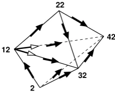
Figure 3: Orientation of edges (‘filled’ arrows) and choice of 2 edges (‘empty’ arrows) of the face shared by two adjacent tetrahedra using the numbering of mesh nodes.
1
3 4
2
ˆ
T
12
32 42 22
T
Figure 4: Using global numbers to examine edges and faces, the ‘structure of orientation’ of T ={12,32,42,22}is the one of ˆT ={1,2,3,4} up to a rotation.
sources are downloaded (from http://www.freefem.org/ff++/) and is thus found in the folderexamples++-load.
4.1
Local implementation strategy for the global assembling
The implementation of edge finite elements is quite delicate. Indeed, basis functions and dofs are associated with the oriented edges of mesh simplices: note that the low order we
and the high orderλkwegenerators change sign if the orientation of the edgeeis reversed. Moreover, recall that forr >1, in order to get a set of linearly independent generators, we also have tochoose2 edges for each facef. Here we wish to construct basis functionslocally, i.e. in each simplex ofTh, in such a way that the contributions coming from simplices sharing edges or faces could be assembled properly inside theglobal matrix of the FE discretization. For this purpose, it is essential to orient in thesame way edges shared by simplices and to choose thesame2 edges for faces shared by adjacent tetrahedra. We have this need also to construct dofs giving the coefficients for the interpolation operator.
This need is satisfied using the global numbers of the mesh nodes (see Fig. 3). More precisely, to orient the edgeseof the basis functions and the vectorste,tf,i, i= 1,2,tT ,i, i=
1,2,3 of the dofs, we go from the node with the smallest global number to the node with the biggest global number. Similarly, to choose 2 edges per face for the face-type basis functions and dofs, we take the 2 edges going out from the node with the smallest global number in the face (and the 1st edge goes to the node with the 2nd smallest global number, the 2nd edge goes to the node with the biggest global number in the face).
Moreover, when we want basis functions ˜wjin duality with the dofs, asecond need should
be satisfied: we wish to usefor all mesh simplices T the ‘dualizing’ coefficients of the matrix ˆ
V−1 calculated, once for all, for the reference simplex ˆT with a certain choice of orientation
and choice of edges (recall thatV−1 already does not depend on the metric of the simplex
for which it is calculated). To be allowed to do this, it is sufficient to use the nodesglobal numbers to decide the order in which the non dualwj (from which we start to then get the
˜
wj) are constructed locally onT. More precisely, for the edge-type (resp. face-type) basis
[image:7.595.189.411.225.320.2]one with the 2nd smallest global number, the 2nd examined edge is from the node with the 1st smallest global number to the one with the 3rd smallest global number, and so on, then the 1st examined face is the one opposite the node with the smallest global number, and so on. Indeed, in this way the first need is respectedand the ‘structure of orientation’ ofT is the one of ˆT up to a rotation (see Fig. 4): then we are allowed to use the coefficients of ˆV−1
for the linear combinations giving the ˜wj.
Note that in 3d (resp. in 2d), to assemble the global linear system matrix, it is not essential which volume-type (resp. face-type) generators are chosen since they are not shared between tetrahedra (resp. triangles). On the contrary, also this choice is important when we want to use for all mesh simplices the coefficients of ˆV−1 calculated for a simplex with a certain choice of orientation and choice of edges.
4.1.1 Implementation of the basis functions
To implement the strategy introduced to construct locally the basis functions ˜wj while
respecting the two requirements just described, two permutations can be used; note that in this paragraph the numberings start from 0, and no more from 1, in order to comply with the C++ plugin written for the insertion in FreeFem++ of the new FE space. First, to construct the non dual wj, we define a permutation pd+1 of d+ 1 elements as follows: pd+1[i] is the local number (it takes values among 0, . . . , d) of the node with thei-th smallest
global number in the simplex T, so we can say that pd+1 is the permutation for which the
nodes of T are listed with increasing global number. For instance, for the tetrahedron T ={12,32,42,22}in Fig. 4, we have p4 ={0,3,1,2}. So, in the first step of construction
of thewj, we replace eachλi appearing in their expression withλpd+1[i]. In the code of the
FreeFem++ plugin, the permutationp4 is calledperm.
Then, in the second step of construction of the ˜wjas linear combinations of thewj, we use
a permutationPndofs ofndofs= dim(W
1
h,r(T)) elements to go back to the local order of edges
and faces. For instance for the tetrahedronT ={12,32,42,22}, the order in which edges are examined in the first step is {{12,22},{12,32},{12,42},{22,32},{22,42},{32,42}}, while the local order of edges would be {{12,32},{12,42},{12,22},{32,42},{22,32},{22,42}}
(the local order is given by how the nodes ofT are listed); similarly, the order in which faces are examined in the first step is{{22,32,42}, {12,32,42},{12,22,42}, {12,22,32}}, while the local order of faces would be{{22,32,42},{12,22,42},{12,22,32},{12,32,42}}. So for this tetrahedron, if r= 2 (for which there are 2 basis functions for each edge and 2 basis functions for each face, 20 basis functions in total listed in Example 1), we have
P20={4,5,0,1, 2,3,8,9,10,11, 6,7; 12,13,18,19,14,15,16,17},
(note that inside each edge or face the 2 related dofs remain ordered according to the global numbers). This permutation (r = 2) is built with the following code. There, edgesMap corresponds to a map that associates the pair{a, b} of nodes of an edgeei with its number
0≤i≤5; this map is rather implemented with an array defined asedgesMap[(a+1)(b+1)] = i, where (a+ 1)(b+ 1) results to be unique and symmetric for a pair (a, b), 0 ≤a, b≤3, representing a tetrahedron edge.
int edgesMap[13] = {-1,-1,0,1,2,-1,3,-1,4,-1,-1,-1,5};
// static const int nvedge[6][2] = {{0,1},{0,2},{0,3},{1,2},{1,3},{2,3}}; int p20[20];
for(int i=0; i<6; ++i) // edge dofs {
int ii0 = Element::nvedge[i][0], ii1 = Element::nvedge[i][1]; int i0 = perm[ii0]; int i1 = perm[ii1];
int iEdge = edgesMap[(i0+1)*(i1+1)]; // i of the edge [i0,i1] p20[i*2] = iEdge*2;
p20[i*2+1] = iEdge*2+1; }
for(int j=0; j<4; ++j) // face dofs {
p20[12+j*2+1] = 12+jFace*2+1; }
Then, we will save the linear combinations of thew`, with coefficients given by thej-th
column of ˆV−1(see Example 1), in the final basis functions ˜w
P20[j], thus in duality with the
chosen dofs. For instance
wtilde[p20[0]] = +4*w[0]-2*w[1]-4*w[16]+2*w[17]-4*w[18]+2*w[19]; wtilde[p20[1]] = -2*w[0]+4*w[1]-2*w[16]-2*w[17]-2*w[18]-2*w[19]; ...
wtilde[p20[18]] = +8*w[18]-4*w[19]; wtilde[p20[19]] = -4*w[18]+8*w[19];
4.2
The interpolation operator
Duality of the basis functions with the dofs is needed in FreeFem++ to provide an interpo-lation operator onto a desired FE space of a function given by its analytical expression (or of a function belonging to another FE space). Indeed, if we define for a (vector) functionu
its finite element approximationuh= Πh(u) using the interpolation operator
Πh:H(curl, T)→Wh,r1 (T), u7→uh= ndofs
X
i=1
ciw˜i, withci:=ξi(u), (8)
we have that, if the duality propertyξj( ˜wi) =δij holds, thenξj(uh) = Pndofs
i=1 ciξj( ˜wi) =cj.
The interpolant coefficientsci =ξi(u) are computed in FreeFem++ with suitable quadrature
formulas (on edges, faces or volumes) to approximate the values of the dofs in Definition 3.2 applied tou.
Now, denote byg the whole integrand inside the dof expression, bynQFi the number of
quadrature points of the suitable quadrature formula (on a segment, triangle or tetrahedron) to compute the integral (of precision high enough so that the integral is computed exactly when the dof is applied to a basis function), and byxp, ap, 1≤p≤nQFi the quadrature
points and their weights. Then we have
ci=ξi(u) = nQFi
X
p=1
apg(xp) = nQFi
X
p=1 ap
d X
j=1
βj(xp)uj(xp), (9)
where for the second equality we have factorized g(xp) in order to put in evidence the d
components ofu, denoted byuj, 1≤j ≤d(see the paragraph below).
Therefore, by substituting the expression of the coefficients (9) in the interpolation op-erator definition (8), we have the following expression of the interpolation opop-erator
Πh(u) = ndofs
X
i=1
nQFi
X
p=1
d X
j=1
apβj(xp)uj(xp) ˜wi= nind X
`=1
α`uj`(xp`) ˜wi`, (10)
where we have set α` equals each apβj(xp) for the right triple (i, p, j) = (i`, p`, j`), and
nind is the total number of triples (i`, p`, j`). Indeed, a FreeFem++ plugin to introduce a
new finite element (represented with a C++ class) should implement (10) by specifying the quadrature points, the indicesi` (dof indices),p` (quadrature point indices),j`(component
indices), which do not depend on the simplex and are defined in the class constructor, and the coefficientsα`, which can depend on the simplex (if so, which is in particular the edge
elements case, theα` are defined with the class functionset).
4.2.1 Interpolation operator for d= 3, r= 2
We report here the code (extracted from the pluginElement Mixte3d.cppmentioned before) defining first the indices of (10) for theEdge13dfinite element, i.e. ford= 3, r= 2. There QFe,QFfare the edge, resp. face, quadrature formulas, andne=6,nf=4, are the number of edges, resp. faces, of the simplex (tetrahedron); we havenind=d·QFe.n·2ne+d·QFf.n·2nf.
int i=0, p=0, e=0; // i is l
for(e=0; e<(Element::ne)*2; e++) // 12 edge dofs {
if (e%2==1) {p = p-QFe.n;}
// if true, the quadrature pts are the ones of the previous dof (same edge) for(int q=0; q<QFe.n; ++q,++p) // 2 edge quadrature pts
for (int c=0; c<3; c++,i++) // 3 components {
this->pInterpolation[i]=p; // p_l this->cInterpolation[i]=c; // j_l this->dofInterpolation[i]=e; // i_l
this->coefInterpolation[i]=0.; // alfa_l (filled with the function set) }
}
for(int f=0; f<(Element::nf)*2; f++) // 8 face dofs {
if (f%2==1) {p = p-QFf.n;}
// if true, the quadrature pts are the ones of the previous dof (same face) for(int q=0; q<QFf.n; ++q,++p) // 3 face quadrature pts
for (int c=0; c<3; c++,i++) // 3 components {
this->pInterpolation[i]=p; // p_l this->cInterpolation[i]=c; // j_l this->dofInterpolation[i]=e+f; // i_l
this->coefInterpolation[i]=0.; // alfa_l (filled with the function set) }
}
Then, the coefficientsα`are defined as follows. We start by writing (9) for one edge-type
dof, withe={n1, n2}:
ci=ξi(u) =
1
|e| Z
e
(u·te)λn1 =
QFe.n
X
p=1
ap(u(xp)·te)λn1(xp)
=
QFe.n
X
p=1 ap
d X
j=1
uj(xp)(xn2j−xn1j)λn1(xp)
so βj(xp) = (xn2j−xn1j)λn1(xp) and α` = ap`βj`(xp`) = (xn2j` −xn1j`)ap`λn1(xp`). Similarly for one face-type dof, withf ={n1, n2, n3},e={n1, n2}:
ci=ξi(u) =
1
|f| Z
f
(u·te) =
QFf.n
X
p=1
ap(u(xp)·te) =
QFf.n
X
p=1 ap
d X
j=1
uj(xp)(xn2j−xn1j)
so βj(xp) = (xn2j −xn1j) and α` = ap`βj`(xp`) = (xn2j` −xn1j`)ap`. The code that generalizes this calculations for all the dofs is the following, extracted from the functionset of the plugin (note that also here we have to pay particular attention to the orientation and choice issues).
int i=0, p=0;
for(int ee=0; ee<Element::ne; ee++) // loop on the edges {
R3 E=K.Edge(ee);
int eo = K.EdgeOrientation(ee); if(!eo) E=-E;
for(int edof=0; edof<2; edof++) // 2 dofs for each edge {
if (edof==1) {p = p-QFe.n;} for(int q=0; q<QFe.n; ++q,++p) {
double ll=QFe[q].x; // value of lambda_0 or lambda_1 if( (edof+eo) == 1 ) ll = 1-ll;
for(int c=0; c<3; c++,i++) {
} } }
for(int ff=0; ff<Element::nf; ff++) // loop on the faces {
const Element::Vertex * fV[3] = {& K.at(Element::nvface[ff][0]), ... // (one unique line with the following)
... & K.at(Element::nvface[ff][1]), & K.at(Element::nvface[ff][2])}; int i0=0, i1=1, i2=2;
if(fV[i0]>fV[i1]) Exchange(i0,i1); if(fV[i1]>fV[i2]) { Exchange(i1,i2);
if(fV[i0]>fV[i1]) Exchange(i0,i1); } // now local numbers in the tetrahedron:
i0 = Element::nvface[ff][i0], i1 = Element::nvface[ff][i1], ... ... i2 = Element::nvface[ff][i2];
for(int fdof=0; fdof<2; ++fdof) // 2 dofs for each face {
int ie0=i0, ie1 = fdof==0? i1 : i2;
// edge for the face dof (its endpoints local numbers) R3 E(K[ie0],K[ie1]);
if (fdof==1) {p = p-QFf.n;}
for(int q=0; q<QFf.n; ++q,++p) // loop on the 3 face quadrature pts for (int c=0; c<3; c++,i++) // loop on the 3 components
{
M.coef[i] = E[c]*QFf[q].a; }
} }
Example 2 (Using the new FEs in a FreeFem++ script). The edge elements in 3d of
degree 2,3 can be used (since FreeFem++ version 3.44) by loading in the edpscript the plugin (load "Element Mixte3d"), and using the keywordsEdge13d,Edge23drespectively. The edge elements of the lowest degree 1 were already available and calledEdge03d. After generating a tetrahedral meshTh, complex vector functionsE,vin, e.g., theEdge03dspace onThare declared with the commands:
fespace Vh(Th,Edge03d); Vh<complex> [Ex,Ey,Ez], [vx,vy,vz];
Then the weak formulation (4) of the problem is naturally transcribed as:
macro Curl(ux,uy,uz) [dy(uz)-dz(uy),dz(ux)-dx(uz),dx(uy)-dy(ux)] // EOM macro Nvec(ux,uy,uz) [uy*N.z-uz*N.y,uz*N.x-ux*N.z,ux*N.y-uy*N.x] // EOM
problem waveguide([Ex,Ey,Ez], [vx,vy,vz], solver=sparsesolver) = int3d(Th)(Curl(Ex,Ey,Ez)’*Curl(vx,vy,vz)) - int3d(Th)(gamma^2*[Ex,Ey,Ez]’*[vx,vy,vz])
+ int2d(Th,in,out)(1i*eta*Nvec(Ex,Ey,Ez)’*Nvec(vx,vy,vz)) - int2d(Th,in)([vx,vy,vz]’*[Gix,Giy,Giz])
+ on(guide,Ex=0,Ey=0,Ez=0);
See more details in the example waveguide.edp available in examples++-load folder of every FreeFem++ distribution. In FreeFem++ the interpolation operator is simply called with the=symbol: for example one can define analytical functionsfunc f1 = 1+x+2*y+3*z; func f2 = -1-x-2*y+2*z; func f3 = 2-2*x+y-2*z;and call[Ex,Ey,Ez]=[f1,f2,f3];.
5
Overlapping Schwarz preconditioners
As shown numerically in [3], the matrix of the linear system resulting from the described high order discretization is ill conditioned. So, when using iterative solvers (GMRES in our case), preconditioning becomes necessary, and here we choose overlapping Schwarz domain decomposition preconditioners.
Consider a decomposition of the domain Ω into Nsub overlapping subdomains Ωs that
of freedom of the whole domain, and letN =SNsubs=1 Ns be its decomposition into the (non disjoint) ordered subsets corresponding to the different (overlapping) subdomains Ωs: a
degree of freedom belongs to Ns if its support (edge, face or volume) is contained in Ωs.
For edge finite elements, it is important to ensure that the orientation of the degrees of freedom is the same in the domain and in the subdomains. Define the matrix Rs as the
restriction matrix from Ω to the subdomain Ωs: it is a #Ns×#N Boolean matrix, whose
(i, j) entry equals 1 if the i-th degree of freedom inNsis thej-th one inN. Note that the
extension matrix from the subdomain Ωsto Ω is given by RTs. To deal with the unknowns
that belong to the overlap between subdomains, define for each subdomain a #Ns×#Ns
diagonal matrixDsthat gives a discretepartition of unity, i.e.
Nsub X
s=1
RTsDsRs=I.
Then theOptimized Restricted Additive Schwarz (ORAS) preconditioner can be expressed as
MORAS−1 =
Nsub X
s=1
RTsDsA−s1Rs, (11)
where the matricesAsare the local matrices of thesubproblems with impedance boundary
conditions (∇ ×E)×n+i˜ωn×(E×n) as transmission conditions at the interfaces between subdomains (note that in this section the term ‘local’ refers to a subdomain and not to a mesh simplex). These local matrices stem from the discretization of the considered Maxwell’s equation by high order finite elements introduced in the previous sections. While the term ‘restricted’ refers to the presence of the partition of unity matricesDs, the term ‘optimized’
refers to the use of impedance boundary conditions (with parameter η = ˜ω in (3)) as transmission conditions, proposed by Despr´es in [17]. The algebraic formulation of optimized Schwarz methods, of the type of (11), was introduced in [25].
The implementation of the partition of unity in FreeFem++ is described in [26]: suit-able piecewise linear functionsχsgiving a continuous partition of unity (
PNsub
s=1 χs= 1) are
interpolated at the barycenters of the support (edge, face, volume) of each dof of the (high order) edge finite elements. This interpolation is obtained thanks to an auxiliary FreeFem++
scalar FE space (Edge03ds0, Edge13ds0, Edge23ds0) that has only the interpolation op-erator and no basis functions, available in the pluginElement Mixte3d mentioned before. When impedance conditions are chosen as transmission conditions at the interfaces, it is essential that not only the functionχsbut also its derivative are equal to zero on the border
of the subdomain Ωs. Indeed, if this property is satisfied, the continuous version of the
ORAS algorithm is equivalent to P. L. Lions’ algorithm (see [27]§2.3.2).
6
Numerical experiments
We validate the ORAS preconditioner (11) for different values of physical and numerical parameters, and compare it with a symmetric variant without the partition of unity (called Optimized Additive Schwarz):
MOAS−1 =
Nsub X
s=1
RTsA−s1Rs.
The numerical experiments are performed for a waveguide configuration in 2dand then in 3d.
6.1
Results for the two-dimensional problem
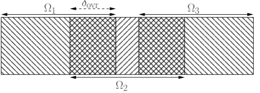
Ω
1Ω
2 [image:13.595.168.433.87.182.2]Ω
3δ
ovrFigure 5: The stripwise decomposition of the two-dimensional domain.
k Ndofs NiterNp Niter max|λ−(1,0)| #{λ∈C\D¯1} #{λ∈∂D1}
0 282 179 5(10) 1.04e−1(1.38e+1) 0(4) 0(12) 1 884 559 6(15) 1.05e−1(1.63e+1) 0(8) 0(40) 2 1806 1138 6(17) 1.05e−1(1.96e+1) 0(12) 0(84) 3 3048 1946 6(21) 1.05e−1(8.36e+2) 0(16) 0(144) 4 4610 2950 6(26) 1.05e−1(1.57e+3) 0(20) 0(220)
Table 1: Influence of the polynomial degreer =k+ 1 on the convergence of ORAS(OAS) preconditioner forω=ω2,Nsub= 2, δovr= 2h.
and σ = 0.15 S m−1. We consider three angular frequencies ω
1 = 16 GHz, ω2 = 32 GHz,
and ω3 = 64 GHz, varying the mesh size h according to the relation h2·ω˜3 = 2 (in [28]
it was proved that this relation avoids pollution effects for the one-dimensional Helmholtz equation).
Note that in 2d the functionEex= (0, e−iγx) verifies the equation, the metallic boundary
conditions on Γw, and the impedance boundary conditions on Γin, Γoutwith parameterη= ˜ω
andgin= (iγ+i˜ω)E
exand gout = (−iγ+i˜ω)Eex; whenσ= 0 we getgin= 2i˜ωEex and
gout = 0. The real part of the propagation constant −iγ gives the rate at which the
amplitude changes as the wave propagates, which corresponds to wave dissipation (note that ifσ >0,<(−iγ)<0, while ifσ= 0,<(−iγ) = 0). A numerical study about the order of (h- andr-) convergence with respect to the exact solution of the high order finite element method can be found in [29].
Here we solve the linear system resulting from the finite element discretization with GMRES (with a stopping criterion based on the relative residual and a tolerance of 10−6),
starting with a random initial guess, which ensures, unlike a zero initial guess, that all frequencies are present in the error. We compare the ORAS and OAS preconditioners, taking a stripwise subdomains decomposition, along the wave propagation, as shown in Fig. 5.
To study the convergence of GMRES preconditioned by ORAS or OAS we vary first the polynomial degree r =k+ 1 (Table 1, Figs. 6–7), then the angular frequencyω (Table 2, Fig. 8, the number of subdomainsNsub (Table 3, Fig. 9) and finally the overlap size δovr
(Table 4, Fig. 10). Here,δovr= 1h,2h,4hmeans that we consider a total overlap between
two subdomains of 1,2,4 mesh triangles along the horizontal direction (see Fig. 5).
In Tables 1–4,Ndofs is the total number of degrees of freedom, NiterNp is the number of
ω Ndofs NiterNp Niter max|λ−(1,0)| #{λ∈C\D¯1} #{λ∈∂D1} ω1 339 232 5(11) 2.46e−1(1.33e+1) 0(6) 0(45) ω2 1806 1138 6(17) 1.05e−1(1.96e+1) 0(12) 0(84) ω3 7335 4068 9(24) 3.03e−1(2.73e+1) 0(18) 0(123)
[image:13.595.122.475.216.297.2] [image:13.595.121.475.660.719.2]Nsub Niter max|λ−(1,0)| #{λ∈C\D¯1} #{λ∈∂D1}
2 6(17) 1.05e−1(1.96e+1) 0(12) 0(84) 4 10(27) 5.33e−1(1.96e+1) 0(38) 0(252) 8 19(49) 7.73e−1(1.96e+1) 0(87) 0(588)
Table 3: Influence of the number of subdomainsNsub on the convergence of ORAS(OAS)
preconditioner fork= 2,ω=ω2,δovr= 2h.
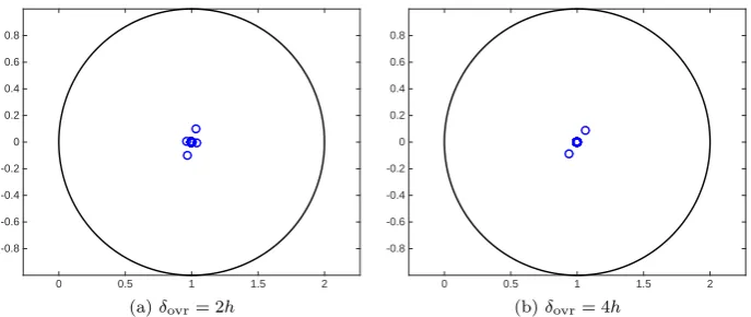
δovr Niter max|λ−(1,0)| #{λ∈C\D¯1} #{λ∈∂D1}
1h 10(20) 1.95e+1(1.96e+1) 3(12) 0(39) 2h 6(17) 1.05e−1(1.96e+1) 0(12) 0(84) 4h 5(14) 1.06e−1(1.96e+1) 0(12) 0(174)
Table 4: Influence of the overlap sizeδovron the convergence of ORAS(OAS) preconditioner
fork= 2,ω=ω2,Nsub= 2.
iterations necessary to attain the prescribed convergence for GMRES without any precon-ditioner, andNiteris the number of iterations for GMRES preconditioned by ORAS (OAS).
Moreover, denoting by
D1={z∈C:|z−z0|<1}
the unit disk centered atz0= (1,0) in the complex plane, we measure also the maximum
dis-tance to (1,0) of the eigenvaluesλof the preconditioned matrix, the number of eigenvalues that have distance greater than 1, and the number of eigenvalues that have distance equal to 1 (up to a tolerance of 10−10). This information is useful to characterize the convergence.
Indeed, if A is the matrix of the system to solve and M−1 is the domain decomposition
preconditioner, thenI−M−1Ais the iteration matrix of the domain decomposition method
used as an iterative solver. So, a measure of the convergence of the domain decomposition solver would be to check whether the eigenvalues of the preconditioned matrixM−1A are
contained inD1. When the domain decomposition method is used, like here, as a
precondi-tioner, the distribution of the spectrum remains a good indicator of the convergence. Note that the matrix of the linear system doesn’t change when Nsub or δovr vary, therefore in
Tables 3–4 (wherek= 2,ω=ω2) we don’t reportNdofs= 1806 and NiterNp = 1138 again.
In all Tables 1–4, we don’t mention the condition number of the preconditioned matrix: indeed, no convergence rate estimates in terms of the condition number of the matrix, as those we are used to with the conjugate gradient method, are available for the GMRES method.
Figs. 6, 8, 9, 10, respectively Fig. 7, show the whole spectrum in the complex plane of the matrix preconditioned by ORAS, respectively by OAS (note that many eigenvalues are multiple), together with ∂D1. We do not report the analogues for the OAS preconditioner
of Figs. 8, 9, 10 because they are quite similar to the configurations in Fig. 7.
Looking at the tables, we can see that the non preconditioned GMRES method is very slow, and the ORAS preconditioner gives much faster convergence than the OAS precondi-tioner. As expected, the convergence becomes slower whenω orNsubincrease, or whenδovr
decreases. In these tests, when varyingk (which gives the polynomial degreer=k+ 1 of the FE basis functions), the number of iterations for convergence using the ORAS precon-ditioner is equal to 5 fork= 0 and then it stays equal to 6 fork >0; this is reflected by the corresponding spectra in Fig. 6, which indeed remain quite similar whenk varies.
Note also that, when using the ORAS preconditioner, for 2 subdomains the spectrum is always well clustered inside the unit disk, except for the case withδovr= 1h(see Fig. 11), in
which 3 eigenvalues are outside with distances from (1,0) equal to 19.5,19.4,14.4. This case δovr= 1hcorresponds to adding a layer of simplices just to one of the two non overlapping
[image:14.595.151.444.191.249.2]0 0.5 1 1.5 2 -0.8
-0.6 -0.4 -0.2 0 0.2 0.4 0.6 0.8
(a)k= 0
0 0.5 1 1.5 2
-0.8 -0.6 -0.4 -0.2 0 0.2 0.4 0.6 0.8
[image:15.595.113.484.113.269.2](b)k= 1,2,3
Figure 6: Influence of the polynomial degree r = k+ 1 on the spectrum of the ORAS-preconditioned matrix forω=ω2, Nsub= 2, δovr= 2h.
-15 -10 -5 0 5 10 15
-25 -20 -15 -10 -5 0
(a)k= 0
-15 -10 -5 0 5 10 15
-25 -20 -15 -10 -5 0
(b)k= 1
-15 -10 -5 0 5 10 15
-25 -20 -15 -10 -5 0
(c)k= 2
-700 -600 -500 -400 -300 -200 -100 0 -450
-400 -350 -300 -250 -200 -150 -100 -50 0 50
D1
(d)k= 3
[image:15.595.118.483.363.696.2]0 0.5 1 1.5 2 -0.8
-0.6 -0.4 -0.2 0 0.2 0.4 0.6 0.8
(a)ω=ω1
0 0.5 1 1.5 2
-0.8 -0.6 -0.4 -0.2 0 0.2 0.4 0.6 0.8
[image:16.595.127.470.110.252.2](b)ω=ω3
Figure 8: Influence of the angular frequencyωon the spectrum of the ORAS-preconditioned matrix fork= 2,Nsub= 2,δovr= 2h.
0 0.5 1 1.5 2
-0.8 -0.6 -0.4 -0.2 0 0.2 0.4 0.6 0.8
(a)Nsub= 4
0 0.5 1 1.5 2
-0.8 -0.6 -0.4 -0.2 0 0.2 0.4 0.6 0.8
[image:16.595.131.471.333.477.2](b)Nsub= 8
Figure 9: Influence of the number of subdomains Nsub on the spectrum of the
ORAS-preconditioned matrix fork= 2,ω=ω2,δovr= 2h.
0 0.5 1 1.5 2
-0.8 -0.6 -0.4 -0.2 0 0.2 0.4 0.6 0.8
(a)δovr= 2h
0 0.5 1 1.5 2
-0.8 -0.6 -0.4 -0.2 0 0.2 0.4 0.6 0.8
(b)δovr= 4h
Figure 10: Influence of the overlap sizeδovr on the spectrum of the ORAS-preconditioned
[image:16.595.126.470.558.703.2]-10 -5 0 5 10 -18
[image:17.595.215.383.85.218.2]-16 -14 -12 -10 -8 -6 -4 -2 0
Figure 11: The spectrum of the ORAS-preconditioned matrix fork= 2,ω=ω2, Nsub= 2, δovr= 1h.
becomes less well clustered. With the OAS preconditioner there are always eigenvalues outside the unit disk. For all the considered cases, we see that the less clustered the spectrum, the slower the convergence.
6.2
Results for the three-dimensional problem
We complete the presentation showing some results for the full 3d simulation, for a waveguide of dimensions c= 0.1004 m, b= 0.00508 m, and a= 0.01016 m. The physical parameters are: ε = 8.85·10−12F m−1, µ = 1.26·10−6H m−1 and σ = 0.15 S m−1 or σ = 0 S m−1. We take a stripwise subdomains decomposition along the wave propagation, with δovr =
2h; however, note that in FreeFem++ very general subdomains decompositions can be considered.
In 3d, if σ= 0 there is an exact solution given by the Transverse Electric (TE) modes:
ExT E = 0,
EyT E =−Cmπ
a sin
mπz
a
cosnπy b
e−iβx,
EzT E =Cnπ
b cos
mπz
a
sinnπy b
e−iβx, m, n
∈N.
The real constant β is linked to the waveguide dimensions a,b by the so called dispersion relation mπa 2+ nπb 2= ˜ω2−β2, and we chooseC=iωµ/(˜ω2−β2). The fieldET E satisfies the metallic boundary conditions on Γwand the impedance boundary conditions on Γin, Γout
with parameterη=β andgin= (iβ+iβ)ET E = 2iβET E andgout= (−iβ+iβ)ET E =0. Since the propagation constant in 3d is β and no more ˜ω, we compute the mesh sizeh using the relationh2·β3 = 1, takingβ =ωβ
√
µε, withωβ= 32 GHz. Then the dispersion
relation gives ˜ω=pβ2+ (mπ/a)2+ (nπ/b)2 (where we choosem= 1, n= 0), and we get ω= ˜ω/√µε.
Again, the linear system is solved with preconditioned GMRES, with a stopping criterion based on the relative residual and a tolerance of 10−6, starting with a random initial guess.
To apply the preconditioner, the local problems in each subdomain of matricesAsare solved
with the direct solver MUMPS [30].
In Tables 5, 6 we show the number of iterations for convergence, for the problem with σ= 0.15 S m−1 andσ= 0 S m−1 respectively, varying first the polynomial degree r=k+ 1
(forNsub= 2), and then the number of subdomainsNsub (fork= 1). Like in the 2d case,
k Ndofs Niter Nsub Ndofs Niter
0 62283 8(40) 2 324654 8(70)
1 324654 8(70) 4 324654 11(106)
[image:18.595.191.404.85.144.2]2 930969 8(99) 8 324654 17(168)
Table 5: Results in 3d, σ = 0.15 S m−1: influence of the polynomial degree r = k+ 1
(forNsub = 2), and of the number of subdomainsNsub (fork= 1), on the convergence of
ORAS(OAS) preconditioner (β=ωβ √
µεwithωβ= 32 GHz,δovr= 2h).
k Ndofs Niter Nsub Ndofs Niter
0 62283 7(40) 2 324654 8(67)
1 324654 8(67) 4 324654 13(114)
2 930969 8(97) 8 324654 23(201)
Table 6: Results in 3d, σ = 0 S m−1: influence of the polynomial degree r = k+ 1 (for Nsub = 2), and of the number of subdomains Nsub (for k = 1), on the convergence of
ORAS(OAS) preconditioner (β=ωβ √
µεwithωβ= 32 GHz,δovr= 2h).
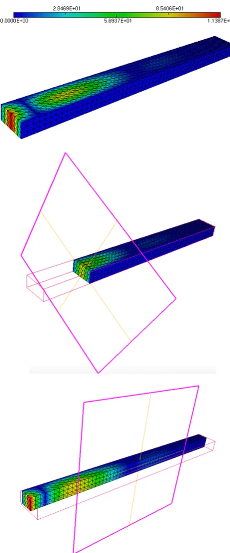
In Figure 12 we plot the norm of the real part of the solution, which decreases as the wave propagates since thereσ= 0.15 S m−1is different from zero.
7
Conclusion
We have adopted a friendly definition of high order edge elements generators and degrees of freedom: both in 2d and 3d their expression is rather simple, and the generators are strictly connected with the degrees of freedom. Their presentation is enriched with illustrative examples, and an operational strategy of implementation of these elements is described in detail. The elements in 3d of polynomial degree 1,2,3 are available in FreeFem++ (since version 3.44), loading the pluginload "Element Mixte3d" and building the finite element spacefespacewith the keywordsEdge03d,Edge13d,Edge23drespectively.
Numerical experiments have shown that Schwarz preconditioning significantly improves GMRES convergence for different values of physical and numerical parameters, and that the ORAS preconditioner always performs much better than the OAS preconditioner. Indeed, the only advantage of the OAS method is to preserve symmetry for symmetric problems: that is why it should be used only for symmetric positive definite matrices as a precondi-tioner for the conjugate gradient method. Moreover, in all the considered test cases, the number of iterations for convergence using the ORAS preconditioner does not vary when the polynomial degree of the adopted high order finite elements increases. We have also seen that it is necessary to take an overlap of at least one layer of simplices fromboth sub-domains of a neighbors pair. All these convergence qualities are reflected by the spectrum of the preconditioned matrix.
Acknowledgement This work was financed by the French National Research Agency (ANR) in the framework of the project MEDIMAX, ANR-13-MONU-0012.
References
[1] A. Bossavit. Computational electromagnetism. Electromagnetism. Academic Press, Inc., San Diego, CA, 1998. Variational formulations, complementarity, edge elements.
[2] R. Hiptmair. Finite elements in computational electromagnetism.Acta Numer., 11:237– 339, 2002.
[3] F. Rapetti. High order edge elements on simplicial meshes.M2AN Math. Model. Numer. Anal., 41(6):1001–1020, 2007.
[4] F. Rapetti and A. Bossavit. Whitney forms of higher degree. SIAM J. Numer. Anal., 47(3):2369–2386, 2009.
[5] M. Ainsworth and J. Coyle. Hierarchic finite element bases on unstructured tetrahedral meshes. Internat. J. Numer. Methods Engrg., 58(14):2103–2130, 2003.
[6] J. Sch¨oberl and S. Zaglmayr. High order N´ed´elec elements with local complete sequence properties. COMPEL, 24(2):374–384, 2005.
[7] R. Hiptmair. Canonical construction of finite elements. Math. Comp., 68(228):1325– 1346, 1999.
[8] J. Gopalakrishnan, L. E. Garc´ıa-Castillo, and L. F. Demkowicz. N´ed´elec spaces in affine coordinates. Comput. Math. Appl., 49(7-8):1285–1294, 2005.
[9] D. N. Arnold, R. S. Falk, and R. Winther. Finite element exterior calculus, homological techniques, and applications. Acta Numer., 15:1–155, 2006.
[10] F. Hecht. New development in FreeFem++. J. Numer. Math., 20(3-4):251–265, 2012.
[11] M. Bonazzoli and F. Rapetti. High-order finite elements in numerical electromagnetism: degrees of freedom and generators in duality. Numerical Algorithms, 74(1):111–136, 2017.
[12] L. E. Garcia-Castillo, A. J. Ruiz-Genoves, I. Gomez-Revuelto, M. Salazar-Palma, and T. K. Sarkar. Third-order N´ed´elec curl-conforming finite element. IEEE Transactions on Magnetics, 38(5):2370–2372, Sep 2002.
[13] S. Reitzinger and J. Sch¨oberl. An algebraic multigrid method for finite element dis-cretizations with edge elements.Numerical Linear Algebra with Applications, 9(3):223– 238, 2002.
[14] J.H. Lai and L.N. Olson. Algebraic multigrid for high-order hierarchicalH(curl) finite elements. SIAM J. Sci. Comput., 33(5):2888–2902, 2011.
[15] A. Toselli. Overlapping Schwarz methods for Maxwell’s equations in three dimensions.
Numer. Math., 86(4):733–752, 2000.
[16] O. G. Ernst and M. J. Gander. Why it is difficult to solve Helmholtz problems with classical iterative methods. InNumerical analysis of multiscale problems, volume 83 of
Lect. Notes Comput. Sci. Eng., pages 325–363. Springer, Heidelberg, 2012.
[17] B. Despr´es, P. Joly, and J. E. Roberts. A domain decomposition method for the har-monic Maxwell equations. InIterative methods in linear algebra (Brussels, 1991), pages 475–484, Amsterdam, 1992. North-Holland.
[19] M. El Bouajaji, V. Dolean, M. J. Gander, and S. Lanteri. Optimized Schwarz methods for the time-harmonic Maxwell equations with dampimg. SIAM J. Scient. Comp., 34(4):2048–2071, 2012.
[20] V. Dolean, M. J. Gander, S. Lanteri, J.-F. Lee, and Z. Peng. Effective transmission conditions for domain decomposition methods applied to the time-harmonic curl-curl Maxwell’s equations. J. Comput. Phys., 280:232–247, 2015.
[21] N. Marsic, C. Waltz, J. F. Lee, and C. Geuzaine. Domain decomposition methods for time-harmonic electromagnetic waves with high-order Whitney forms. IEEE Transac-tions on Magnetics, 52(3):1–4, March 2016.
[22] M. Bonazzoli, V. Dolean, F. Rapetti, and P.-H. Tournier. Parallel preconditioners for high-order discretizations arising from full system modeling for brain microwave imaging. International Journal of Numerical Modelling: Electronic Networks, Devices and Fields, pages e2229–n/a, 2017. e2229 jnm.2229.
[23] P. Monk. Finite element methods for Maxwell’s equations. Numerical Mathematics and Scientific Computation. Oxford University Press, New York, 2003.
[24] J.-C. N´ed´elec. Mixed finite elements in R3. Numer. Math., 35(3):315–341, 1980.
[25] A. St-Cyr, M. J. Gander, and S. J. Thomas. Optimized multiplicative, additive, and restricted additive Schwarz preconditioning. SIAM Journal on Scientific Computing, 29(6):2402–2425, 2007.
[26] P.-H. Tournier, I. Aliferis, M. Bonazzoli, M. de Buhan, M. Darbas, V. Dolean, F. Hecht, P. Jolivet, I. El Kanfoud, C. Migliaccio, F. Nataf, C. Pichot, and S. Semenov. Microwave Tomographic Imaging of Cerebrovascular Accidents by Using High-Performance Com-puting. preprint, submitted, 2016.
[27] V. Dolean, P. Jolivet, and F. Nataf.An Introduction to Domain Decomposition Methods: algorithms, theory and parallel implementation. SIAM, 2015.
[28] F. Ihlenburg and I. Babuˇska. Finite element solution of the Helmholtz equation with high wave number. I. The h-version of the FEM. Comput. Math. Appl., 30(9):9–37, 1995.
[29] M. Bonazzoli, E. Gaburro, V. Dolean, and F. Rapetti. High order edge finite element approximations for the time-harmonic Maxwell’s equations. In2014 IEEE Conference on Antenna Measurements Applications (CAMA) Proceedings, November 2014.
[30] P. Amestoy, I. Duff, J. L’Excellent, and J. Koster. A fully asynchronous multifrontal solver using distributed dynamic scheduling. SIAM Journal on Matrix Analysis and Applications, 23(1):15–41, 2001.
[31] P. Jolivet, F. Hecht, F. Nataf, and C. Prud’Homme. Scalable domain decomposition preconditioners for heterogeneous elliptic problems. InProc. of the Int. Conference on High Performance Computing, Networking, Storage and Analysis, pages 1–11. IEEE, 2013.