A Predictive Resource Allocation Algorithm in the
LTE Uplink for Event Based M2M Applications
Jason Brown, Member IEEE and Jamil Y Khan, Senior Member IEEE
School of Electrical Engineering and Computer Science The University of Newcastle
Callaghan, NSW 2308, AUSTRALIA
Email: [email protected], [email protected]
Abstract— Some M2M applications such as event monitoring involve a group of devices in a vicinity that act in a co-ordinated manner. An LTE network can exploit the correlated traffic characteristics of such devices by proactively assigning resources to devices based upon the activity of neighboring devices in the same group. This can reduce latency compared to waiting for each device in the group to request resources reactively per the standard LTE protocol. In this paper, we specify a new low complexity predictive resource allocation algorithm, known as the one way algorithm, for use with delay sensitive event based M2M applications in the LTE uplink. This algorithm requires minimal incremental processing power and memory resources at the eNodeB, yet can reduce the mean uplink latency below the minimum possible value for a non-predictive resource allocation algorithm. We develop mathematical models for the probability of a prediction, the probability of a successful prediction, the probability of an unsuccessful prediction, resource usage/wastage probabilities and mean uplink latency. The validity of these models is demonstrated by comparison with the results from a simulation. The models can be used offline by network operators or online in real time by the eNodeB scheduler to optimize performance.
Index Terms— LTE, M2M, predictive scheduling, proactive scheduling, OPNET.
I.INTRODUCTION
The 3GPP Long Term Evolution (LTE) standard provides packet based mobile broadband services with high data rates, low latency, high spectral efficiency, flexible bandwidth allocations and low cost compared to earlier wide area mobile wireless standards [1]. Although LTE can transport any type of payload in theory, the system nevertheless includes optimisations for certain traditional Human-to-Human (H2H) telecommunications services. For example, optimisations for voice are included via Semi-Persistent Scheduling (SPS) [2] and TTI Bundling [3]. In addition, the dimensioning of the downlink resource assignment control channel implicitly assumes the prevalence of traditional telecommunications services such as web browsing in which data packets are typically medium or large in size [4], otherwise the system capacity becomes control channel rather than data channel limited.
In spite of the initial design focus of LTE on traditional telecommunications services, there has been significant interest in deploying Machine-to-Machine (M2M) applications over
existing LTE networks and extending LTE to better support M2M services and features [5][6]. These M2M applications relate to various industries such as automotive, utility and healthcare and typically involve communication between devices or between devices and servers with little or no human input. Some of the unique challenges of M2M services include a relatively large number of devices sending data infrequently, typically small packet sizes, diverse QoS requirements between different applications and typically low mobility [7]. One of the most intriguing aspects of M2M applications is that neighbouring devices pertaining to a group may act together in some fashion to achieve an objective [8]. For example, for a group of related M2M devices such as sensors in a Wireless Sensor Network (WSN), the fact that one sensor has triggered may increase the probability that other sensors in the vicinity may also trigger in quick succession. This is completely different from traditional telecommunications services in which the traffic characteristics of each device are typically regarded as independent of those of any other device.
In this paper, we demonstrate how the correlated uplink traffic patterns associated with a group of M2M devices can be exploited by the LTE eNodeB scheduler to reduce uplink latency. In particular, when one device in the group requests uplink resources, the eNodeB can employ certain criteria to determine whether to proactively assign uplink resources to neighboring devices in lieu of waiting for those neighboring devices to reactively request uplink resources according to the standard LTE resource request protocol. This can reduce end-to-end uplink latency at the potential expense of wastage when resources are allocated proactively either too early (i.e. before a device has data to send) or when a device has no data to send at all. This concept of proactive/predictive resource allocation is very important because while the LTE uplink is designed to support a data plane latency of less than 10ms [1], typical latencies can be significantly higher depending upon the system configuration, load, packet size and channel conditions [9], yet certain M2M applications are extremely delay sensitive [10][11].
report the arrival of the disturbance. Generalizations to a scattered 2D or 3D topology of devices are possible, but are not considered in this paper. In addition, more complex predictive
resource algorithms can be devised such as a two way
algorithm that allows predictive resource allocations to be made in both forward and reverse directions, but these are significantly more difficult to model via a theoretical analysis, therefore we concentrate on the one way algorithm as a baseline for performance improvements in this paper. We characterize the one way algorithm via a mathematical analysis of metrics such as the probability of a prediction, the probability of a successful prediction, the probability of an unsuccessful prediction, resource usage/wastage probabilities and mean uplink latency. The theoretical mathematical models are validated via simulation results from a bespoke LTE OPNET simulation model.
The mathematical models for predictive resource allocation have application beyond simple characterization of algorithm performance. For instance, they can be employed offline by network operators to configure the aggressiveness of a prediction strategy as a compromise between reduced latency and wasted resources (which occur as the result of unsuccessful predictions), assuming the characteristics of the group traffic profile are known. Alternatively, they can be employed online by the eNodeB to estimate certain characteristics of the group traffic profile (e.g. the speed of disturbance propagation) in real time in order to modify the algorithm parameters dynamically for optimum performance. We only consider these applications briefly in this paper, but they demonstrate the potential utility of the models.
The literature includes some related work. In [12], we specified a related predictive resource allocation algorithm for the LTE uplink and provided simulation results, but a mathematical analysis was not conducted. In [13], a predictive scheduling algorithm for uplink traffic in WiMAX networks is described which attempts to reduce latency for the real time polling service (rtPS) based upon analysis of the bandwidth request queues at the base station, although this work does not exploit the correlated traffic patterns between neighbor devices. In [14-16], the authors define proactive resource allocation for wireless networks at the single user level in order to afford delay and capacity gains. In contrast, our work addresses predictive resource allocation at the multi-user/device single group level. In [17], the authors examine predictive resource allocation using time series models for cognitive networks, but again this work does not address the correlated traffic patterns between devices.
The principal contributions of this paper are as follows:
Specification of a new low complexity predictive
resource allocation algorithm, known as the one way algorithm, for use with delay sensitive event based M2M applications in the LTE uplink. This algorithm requires minimal incremental processing power and memory resources at the eNodeB, yet can reduce the mean uplink latency significantly below the minimum possible value for a non-predictive resource allocation algorithm.
Characterization of the performance of the one way
algorithm with mathematical models.
Validation of the models via an OPNET based
simulation.
Explanation of the utility of the models in offline and online algorithm optimization.
The remainder of this paper is organized as follows. In Section II, we review the existing reactive uplink resource allocation mechanism in LTE. Section III introduces predictive resource allocation concepts. Section IV is concerned with the one way predictive resource allocation algorithm that is the principal topic of this paper; it specifies the algorithm, presents the mathematical analysis and validates the theoretical model against simulation results. The utility of the mathematical models in offline and online optimization of the algorithm is briefly discussed in Section V. Section VI provides additional insights including the analysis of more general disturbance models and the effect of a fully loaded network on the prediction performance. We provide conclusions and recommendations for further work in Section VII.
II.LTEREACTIVE UPLINK RESOURCE ALLOCATION
As with the research outlined in [12], we consider the RRC_CONNECTED state [18] of LTE device operation, which is the high energy state. In some scenarios, it is unlikely that all devices in a group would remain in the RRC_CONNECTED state for an extended period of time. However, there are M2M application scenarios where this can be justified, for example in a Smart Grid where devices are externally powered and latency is a critical factor for control and protection. Additionally, even when devices normally reside in the RRC_IDLE state, there may be occasions where they are proactively migrated to the RRC_CONNECTED state in anticipation of some event.
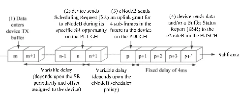
Fig. 1 illustrates the standard uplink latency components for an LTE device in the RRC_CONNECTED state assuming the Frequency Division Duplexing (FDD) mode of LTE operation. A device sends a Scheduling Request (SR) message [19] to inform the eNodeB that it has data to send and request scheduling for this data. The device must wait for its individual pre-assigned offset subframe within an SR period, , to send its SR. Therefore the time required for a device to send its SR from the first available subframe after the data enters the transmit buffer is a discrete random variable with a uniform distribution over the interval (1, ). is a system configuration variable with allowed values 5, 10, 20, 40 and 80 subframes [20] (where each LTE subframe is 1ms in duration) with higher values usually employed to support a large number of devices as in an M2M deployment. With = 80 subframes, the mean delay from this component alone is (1+80)/2 = 40.5ms which is far higher than the design goal of 10ms.
its uplink scheduling grant from the eNodeB, the grant applies to a fixed offset of 4 subframes or 4ms in the future for an LTE FDD system [20]. Therefore, the minimum uplink latency is 6ms which assumes that, by chance, the SR is sent in the very next subframe after the data packet enters the device buffer.
Fig. 1: Uplink Latency Components in LTE FDD
III.PREDICTIVE UPLINK RESOURCE ALLOCATION
The eNodeB can exploit the correlated uplink traffic patterns between related devices of a group in an M2M application to reduce latency. In particular, when one device in the group sends an SR, and the time to the next SR opportunity for a neighbor device in the same group is, by chance, greater than some threshold , the eNodeB can proactively use predictive resource allocation to grant this neighbor device resources to send its packet(s) ahead of its regular SR opportunity, thereby reducing latency. Of course, there is a risk with unsolicited predictive resource allocation that resources will be assigned to a device before it has a packet to send, if it has a packet to send at all, and therefore, to some extent, there is a compromise between latency reduction and resource wastage. Ultimately the requirements of the application dictate the aggressiveness of the predictive resource allocation (as determined by the parameter ).
Fig. 2 illustrates the concept of predictive uplink resource allocation. Devices A, B, C and D are members of the same group (e.g. sensors in a WSN). Device A is the first to send an SR based upon a disturbance, although not necessarily the first device to compose a data packet for transmission based upon the event (that is device B in the Fig. 2). Devices B, C and D are neighbors of device A based upon some metric (usually distance between devices) and must be labelled as such in the eNodeB in order to facilitate predictive resource allocation since predictions are targeted at specific devices which are likely to have pending data to minimise resource wastage. This could be done via static provisioning or a dynamic registration protocol, the latter probably requiring standardization.
We assume through the paper that although each device has a periodic SR opportunity every subframes, the offset of that SR opportunity within the period is assigned randomly by the eNodeB. In particular, we assume the eNodeB does not intentionally assign similar offsets to devices which are neighbors in an attempt to allow those devices to send SRs in quick succession when an event occurs. Such a design will in general afford no advantage (and can be counter-productive)
[image:3.595.45.289.178.274.2]unless the speed and direction of the event propagation are known in advance. In the example of Fig. 2, we see that the SR opportunities of the four devices are spread across the SR period without any intentional ordering or staggering even though devices B, C and D are neighbors of device A.
Fig. 2: Predictive Uplink Resource Allocation Concept
The eNodeB employs the standard reactive uplink resource allocation for device A since it is the first device to indicate that uplink data is pending. However, once the eNodeB has received the SR from device A, it determines which of its neighbors should be subject to predictive resource allocation. This is based upon the interval to the next SR opportunity for each neighbor. If this interval is greater than a certain threshold
of subframes, where , the eNodeB predictively
allocates resources for the neighbor ahead of the regular SR opportunity for that neighbor. The predictive resource allocation is such that it will not occur earlier than subframes following receipt of the SR from device A.
Referring to Fig. 2, for neighbor device B, the next SR opportunity occurs less than subframes after the SR was received from device A; therefore the eNodeB does not issue a predictive uplink grant and the uplink resource allocation occurs normally.
For neighbor device C, the next SR opportunity occurs more than subframes after the SR was received from device A; therefore the eNodeB issues a predictive uplink grant for device C, in this case exactly subframes after the SR was received from device A. There is pending uplink data for device C at the time the predictive resource allocation is made, and this data is transmitted a fixed interval of 4 subframes (4ms) after the predictive uplink grant is received. Therefore, for device C, the predictive resource allocation is successful and the device does not transmit an SR at its next SR opportunity (since there is no data to transmit at the time of this opportunity). Clearly latency is reduced compared to the standard reactive LTE resource allocation model in which the device waits for its next SR opportunity before indicating to the eNodeB that it has pending data. Note that because the predictive resource allocation is achieved without sending an SR, the minimum possible uplink latency is reduced from 6ms to 5ms.
For neighbor device D, the next SR opportunity occurs more than subframes after the SR was received from device A; therefore the eNodeB issues a predictive uplink grant for
time
t1 t1+σ
y
device A device B device C device D
Data arrives in device Tx buffer SR opportunity: SR sent SR opportunity: SR not sent
device D, in this case at more than subframes after the SR was received from device A (for example due to scheduling congestion). There is no pending uplink data for device D at the time the predictive resource allocation is made, and therefore the predictive resource allocation is unsuccessful/wasted. Instead device D sends an SR at its next available SR opportunity (because data arrives after the predictive resource allocation is made) and the uplink resource allocation follows the normal path.
Expanding further on the case of device D, we note that as any uplink allocation in LTE (whether predictive or normal) implies that the target device sends data a fixed interval of 4ms in the future after receiving the grant, there is the possibility that a high performance device may be able to send a data packet which arrives in its transmit buffer up to 4ms after the predictive uplink grant is received from the eNodeB. We do not consider such high performance devices in this paper. The criterion we adopt is that, in order for a device to send a data packet as part of a predictive resource allocation, the data packet must already be present in the device transmit buffer before the predictive uplink grant is received from the eNodeB. Devices B and D send SRs that can be used by the eNodeB as the basis of further predictive resource allocations for the neighbors of those devices. Device C does not send an SR as it transfers its packet via a successful predictive resource allocation; in this case, the data packet received as part of the predictive resource allocation can be used by the eNodeB to trigger further predictive resource allocations. We refer to this feature as chaining of predictions and it was part of the algorithm employed in [12]; however, for this paper, we do not consider chaining further as it does not lend itself to a tractable mathematical analysis.
As discussed in [12], predictive uplink resource allocation is not expected to require major changes to 3GPP standards.
IV.ONE WAY PREDICTION
A.Algorithm
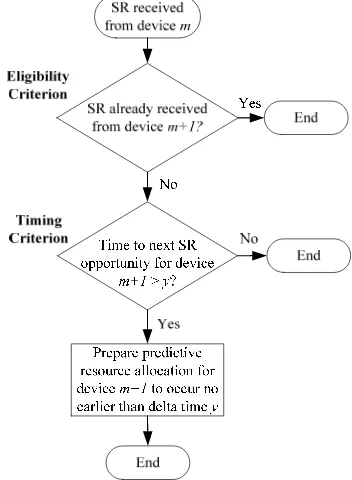
Fig. 3 specifies the functionality of the one way eNodeB predictive uplink resource allocation algorithm analysed in this section. An example application context of this algorithm is a line of sensors along which a disturbance is travelling.
For this algorithm, predictive resource allocations only occur in one direction i.e. in the direction from device m to m+1, and we assume in the following analysis that this is the same direction as the disturbance propagation, which results in superior performance. However, since devices do not in general send SRs with the same timing or sequence as the disturbance reaches them (because they have to wait a random amount of time until their next SR opportunity once a data packet is pending), it is possible to generate successful predictions with this algorithm even when the direction of disturbance propagation is opposite to that of the prediction. Clearly more complex predictive resource algorithms can be devised such as a two way algorithm that allows predictive resource allocations to be made in both forward and reverse directions, but these are significantly more difficult to model via a theoretical analysis, therefore we concentrate on the one
[image:4.595.346.522.114.354.2]way algorithm as a baseline for performance improvements in this paper.
Fig. 3: One Way Predictive Uplink Resource Allocation Algorithm
In Fig. 3, the eNodeB targets device m+1 for a predictive resource allocation if and only if two criteria are satisfied. Firstly, the eligibility criterion dictates that device m+1 is only eligible for a predictive resource allocation if it has not sent an SR recently (i.e. as determined by a configurable timer), since otherwise the eNodeB will already be in the process of scheduling (or have scheduled) a data transfer for this device. Secondly, the timing criterion dictates that the time remaining to the next SR opportunity for device m+1 is greater than parameter at the time the SR from device m is received, otherwise there is little to be gained (in terms of reduced data transfer latency) by performing a predictive resource allocation. If both the eligibility and timing criteria are satisfied when an SR is received from device m, the eNodeB will schedule a predictive resource allocation targeting device m+1 to occur no earlier than subframes in the future. If this predictive resource allocation is successful, device m+1 will not send an SR as part of its uplink data transfer and therefore there cannot be a predictive resource allocation targeting device m+2.
B.Probability of a Prediction
We first consider the probability of the eNodeB
targeting a predictive resource allocation towards device m+1 given it has received an SR from device m, where device m+1 is downstream from device m with respect to the disturbance propagation. Exploiting the fact that device m will send an SR within one SR period of detecting the disturbance, and using the total law of probability, this is as follows:
where:
is the Scheduling Request (SR) period configured by the eNodeB.
is a random variable representing the first
subframe that device m is scheduled to send its SR after the disturbance has reached it.
is the subframe after the disturbance has reached
device m, where 1 and 1.
We consider the case for which ~ , where
, represents the discrete uniform distribution between
and inclusive so that 1 σ⁄ . Then Eq. (1)
becomes:
1
| (2)
In order to find an expression for | , we
[image:5.595.309.552.332.455.2]consider Fig. 4 which shows the relative SR timing for device m and device m+1. The disturbance takes subframes (where is assumed to be an integer for this analysis) to travel between device m and device m+1. Once the disturbance has reached a device, the device will send an SR within the next subframes according to its assigned SR offset within the SR period unless that device is the target of a successful predictive resource allocation. The window of subframes in which each device can possibly send an SR is illustrated by the respective rectangle in Fig. 4.
Fig. 4: SR Timing for Adjacent Devices
There are two cases to consider. In the first case, in which
device m sends its SR such that (for example
in Fig. 4), the eligibility criterion for a predictive resource allocation is automatically satisfied because device m+1 cannot send its SR until subframe at the earliest per Fig. 4. The probability of a predictive resource allocation then
only depends on the timing criterion. Considering ,
device m+1 will have precisely one SR opportunity between subframes and inclusive (since that defines an interval of subframes), and the timing criterion is only satisfied if the time to that next SR opportunity for device m+1 is greater than i.e. if the SR opportunity occurs at subframe or later. Therefore the probability that the timing criterion is satisfied, or equivalently the probability of a predictive resource
allocation occurring, at the time when the SR from
device m is received is 1 /
1 ⁄ assuming a uniform and independent
distribution of SR opportunities across the device population. In the second case, in which device m sends its SR such that
, the eligibility criterion for a predictive resource allocation is not automatically satisfied. For example, if in Fig. 4, the eligibility criterion is not necessarily satisfied because device m+1 will already have sent an SR if it had a previous SR opportunity between and . Therefore, considering , the eligibility criterion is only satisfied if device m+1 has an SR opportunity between subframes and . This is because if the next SR opportunity occurs later
than subframe , there would have been an earlier SR
opportunity ( subframes earlier) during which an SR would already have been sent by device m+1. As in the previous case, the timing criterion is only satisfied if the time to the next SR opportunity for device m+1 is greater than i.e. if the SR
opportunity occurs at subframe or later. Therefore the
probability of a predictive resource allocation occurring is
1 / ⁄ when .
In summary, we have:
|
1 ,
,
(3)
Consolidating Eq. (2) and Eq. (3) for yields:
1 1 1
(4)
We note that the 2nd summation corresponds to the sum of
an arithmetic progression and therefore:
1 1
2
1
2
1 2 1
2
(5)
When consolidating Eq. (2) and Eq. (3) for , the upper
limit of is reduced from to 1 because, with
reference to Fig. 4, the latest possible SR opportunity for device m+1 is at subframe and therefore the latest SR opportunity for device m that can give rise to a predictive resource allocation targeting device m+1 occurs at subframe
. Therefore, for :
1 1 1
(6)
[image:5.595.44.288.433.532.2]1 1 2
1 2
2
(7)
In summary, we have:
1 2 1
2 ,
1 2
2 ,
(8)
C.Probability of a Successful/Unsuccessful Prediction
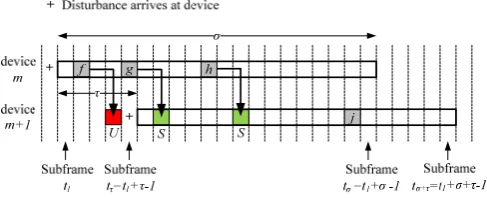
[image:6.595.44.288.325.424.2]We now consider the probability of the eNodeB targeting a successful predictive resource allocation, denoted by the event , and an unsuccessful predictive resource allocation, denoted by the event , towards device m+1 given it has received an SR from device m. Fig. 5 demonstrates how successful and unsuccessful predictions occur for 2 which in this example is less than the inter-device disturbance propagation time .
Fig. 5: Successful and Unsuccessful Predictions for y=2
In Fig. 5, , and are the subframes corresponding to alternative SR opportunities for device m which all result in a predictive resource allocation targeting device m+1 because the eligibility and timing criteria are satisfied in each case when the SR opportunity for device m+1 occurs during subframe . An unsuccessful predictive resource allocation occurs when the predictive resource allocation occurs prior to or during the subframe when the disturbance reaches the target device (see the example SR opportunity for device m which occurs during subframe ) since the target device has no data to send, while a successful predictive resource allocation occurs when the predictive resource allocation occurs post the disturbance reaching the target device (see the example SR opportunities for device m which occur during subframes and ).
From this discussion, it is clear that an unsuccessful
predictive resource allocation can only occur for and
when there is a predictive resource allocation under the
constraint . Therefore, with reference to Eq. (2) and
Eq. (3):
1
| 1 1
1
2
(9)
In summary, we have:
1
,
0 , (10)
The probability of a successful predictive resource allocation is given by subtracting Eq. (10) from Eq. (8) thus:
1 1
2 ,
1 2
2 ,
(11)
D.Probability of Sending an SR for Data Transfer
The probability of device m+1 sending an SR as
part of its data transfer given the eNodeB has received an SR from device m is of interest because an SR consumes resources on the Physical Uplink Control Channel (PUCCH) [20] as illustrated in Fig. 1. Device m+1 sends an SR only when there is either no prediction or an unsuccessful prediction targeted towards it. Therefore:
1 1 (12)
E.Expected Delay
In this section, we derive an expression for the expected delay of device m+1 sending its data packet given the eNodeB has received an SR from device m for the case of
. This considers all possible scenarios i.e. no prediction, a successful prediction and an unsuccessful prediction targeting device m+1. We assume that the system is lightly loaded so that scheduling can occur at the earliest possible opportunity. In this sense, the derived expression is a best case estimate, but importantly it shows the dependence upon the parameter .
Using the total law of expectation and again considering the
case where ~ , , we can write:
|
1
|
(13)
The delay clearly depends upon whether there is a successful prediction , unsuccessful prediction or no prediction at all. Therefore we split Eq. (13) into three corresponding components as follows:
Γ Γ Γ
where:
Γ 1 | ,
Γ 1 | ,
Γ 1 | ,
For a successful prediction , the predictive resource allocation targeting device m+1 takes place at the earliest
during subframe (i.e. subframes after the SR from
device m is received by the eNodeB during subframe ), yet the disturbance reached device m+1 during subframe (see Fig. 4). Therefore the lowest delay for the predictive resource
allocation is , and the expected
end-to-end data transfer delay | ,
where 4.5 subframes for LTE FDD and represents the
combined delay contribution of the disturbance arriving on average midway through subframe (0.5 subframes) and, as illustrated in Fig. 1, the fixed delay of 4 subframes between device m+1 receiving the resource allocation and sending the data.
We employ Eq. (3) as the basis for , but note that a
successful prediction can only occur for as
discussed in Section IV.C. Then Γ from Eq. (14) is
determined as follows:
Γ 1 1
1
(15)
Simplifying Eq. (15) using results for the sum of an arithmetic progression leads to:
Γ 1 2 1
2
2 1
2
(16)
where is the nth square pyramidal number given by:
1 2 1
6 (17)
For an unsuccessful prediction , the predictive resource allocation targeting device m+1 again takes place at the earliest during subframe , but this is before or during the subframe when the disturbance reaches this device (see Fig. 5). Once the disturbance arrives at device m+1, this device therefore follows the normal reactive resource request procedure and sends an SR during its next SR opportunity. Given that a prediction has already taken place for device m+1, its next SR opportunity is by definition more than subframes after the subframe in which the SR from device m was received, so
there are only 1 possible subframes in which the SR
for device m+1 can be sent. The basic range for these
1 subframes is … (with SR delay
… or 1 … 1 inclusive.
However, the SR can only be sent after subframe when the
disturbance arrives, so subframes at
the start of the range which do not occur after are mapped to the subsequent SR opportunity subframes later with a corresponding increase in SR delay. Therefore the expected SR
delay is:
1 1 1
2
1
2 2 1
(18)
The additional delay components contributing to
| , are 1 subframe for the uplink grant and
4.5 subframes for the combined contribution of the
disturbance arriving on average midway through subframe (0.5 subframes) and, as illustrated in Fig. 1, the fixed delay of 4
subframes between device m+1 receiving the resource
allocation and sending the data. Building on Eq. (9), Γ from Eq. (14) is therefore determined as follows:
Γ 1
2 2 1 1
1
(19)
Simplifying Eq. (19) leads to:
Γ 1 1 1
2
1 1 (20)
For the case of no prediction , given that the SR from device m is received by the eNodeB during subframe , device m+1 must have already sent its SR (according to the eligibility criterion of Fig. 3) or it must send its SR within the next
subframes i.e. on or before subframe (according to the
timing criterion of Fig. 3), otherwise a predictive resource allocation would occur. With reference to Eq. (3), the
probability of no prediction is 1 / for
and / for .
For , all 1 nominal SR opportunities
… inclusive for device m+1 occur no later than when the disturbance has reached this device during subframe (see Fig. 5), and therefore the actual SR opportunities lie one SR
period or subframes later during the range …
(with SR delay … or …
inclusive. Therefore the expected SR delay is
/2.
For , the nominal SR opportunities for device
m+1 are … (with SR delay … or
… inclusive. However, of these 1 nominal
the start of the range which do not occur after subframe (when the disturbance reaches device m+1) are mapped to the subsequent SR opportunity subframes later with a corresponding increase in SR delay. Therefore the expected SR
delay is:
1
2 1
1
2
1 1
(21)
For , the eligibility criterion is not
automatically satisfied since device m+1 can send its SR after subframe before the SR from device m is sent at subframe , so this must be taken into account as well as the timing criterion. If either criterion is not satisfied, a prediction does not take place. The SR opportunities for device m+1 are
… (with SR delay … or 1 …
inclusive where the lower limit is determined by the eligibility criterion and the upper limit by the timing criterion.
The expected SR delay is then 1 /2.
The additional delay components contributing to
| , are 1 subframe for the uplink grant and
4.5 subframes associated with the normal reactive LTE uplink resource allocation. Γ from Eq. (14) is therefore determined as follows:
Γ 1 2 1 1
1
2
1
1 1
1
1 1
2 1
(22)
Simplifying Eq. (22) yields:
Γ 1 2 3 2
2 2
1 3 2
2 2
3 2 2 1
4 2
2 2
(23)
F.Expected Delay
In this section, we derive an expression for the expected
delay of device m+1 sending its data packet given the
eNodeB has received an SR from device m for the case of . This considers all possible scenarios i.e. no prediction and successful prediction targeting device m+1. Unsuccessful
predictions are not possible for as illustrated by Eq.
(10). Again we assume that the system is lightly loaded so that
scheduling can occur at the earliest possible opportunity.
Similar to Eq. (14), we represent as the summation of
two components, one for a successful prediction and one for no prediction , as follows:
Γ Γ
where:
Γ 1 | ,
Γ 1 | ,
(24)
Using arguments similar to those in Section IV.E for a successful prediction , and building on Eq. (6) for the probability of a prediction (which is equivalent to the probability of a successful prediction when ), we obtain:
Γ 1 1
1 (25)
Simplifying Eq. (25) using results for the sum of an arithmetic progression leads to:
Γ 1 22 2 1
1 1
2
(26)
where is the nth square pyramidal number given by Eq. (17).
Using arguments similar to those in Section IV.E for the case of no prediction , we obtain:
Γ 1 2 1 1 1 1
1 1
2 1
1 1
2 1
(27)
For 1 , corresponding to the third
summation in Eq. (27), the probability of a prediction is zero (and therefore the probability of no prediction
is one) because, with reference to Fig. 5,
i.e. the last SR opportunity for device m+1 during subframe occurs no later than subframes after device m sends its SR during subframe , so the timing criterion for predictive resource allocation cannot be satisfied. In this case, the
expected packet delay | , is the expected
opportunities are possible) plus 1 subframe for the uplink grant plus 4.5 subframes. Simplifying Eq. (27) leads to:
Γ 1 3 2
2
1
2
3 2 1
4 2
1 3 2
2
(28)
G.Validation
[image:9.595.298.559.114.239.2]An OPNET based simulation using a bespoke model for the LTE eNodeB was executed to validate the one way theoretical models of Section IV.B through Section IV.F for various values of the parameter . The simulation parameters are listed in Table I.
Table I: Simulation Parameters
Parameter Value
Frequency Band 3GPP Band 1 [21] (1920MHz
uplink / 2110MHz downlink)
Mode FDD
Channel bandwidth 2x5MHz
Cyclic prefix type Normal
Maximum device Tx power 1W
Maximum eNodeB Tx power 5W
Device Rx sensitivity -110dBm
eNodeB Rx sensitivity -123dBm
Device antenna gain 4dBi
eNodeB antenna gain 9dBi
Device height 1.5m
eNodeB height 40m
SR periodicity 20ms, 40ms and 80ms
PUCCH channels 2
Channel models Suburban fixed Erceg model with
Terrain Type C [22]
HARQ Supported
Radio access network model Single cell, 5km radius (78.5km2)
Uplink traffic model 200 sensors equally spaced along a
line. Each sensor sends an alarm when a disturbance reaches it.
Packet size 32 bytes (application layer)
60 bytes (IP layer)
QoS for uplink/downlink traffic Best effort on default bearer
Uplink/downlink scheduler algorithm
Dynamic fairness (initial uplink allocation of 504 bits at the
application layer)
Inter-sensor propagation time 5ms, 10ms and 20ms
For each simulation run, a disturbance travelled unidirectionally along a line of 200 equally spaced sensors/devices and each sensor sent an alarm when the disturbance reached it. The sequence of prediction outcomes was recorded and statistics collected based upon this sequence as specified in Table II. The trigger for the statistics update was always a successful predictive resource allocation (at device
m-1 in Table II) because the following downstream device
[image:9.595.59.240.122.195.2](device m) is never a target for a predictive resource allocation, allowing an assessment of whether a predictive resource allocation occurs for the next downstream device (device m+1) or not in which the theoretical assumption that the SR opportunities for device m are uniformly distributed across an SR period is valid.
Table II: Calculation of Statistics During Simulation Involving One Way Prediction
Device m-1
Device m
Device m+1
Action
S SR X Increment number of prediction
opportunities
S SR SR Increment number of SRs sent
S SR Pred Increment number of predictions
S SR S Increment number of successful predictions
S SR U Increment number of unsuccessful predictions
(SR = scheduling request, Pred = prediction, S = successful prediction, U = unsuccessful prediction, X = do not care)
Note that the rows of Table II are not mutually exclusive, so when, for example, an unsuccessful predictive resource
allocation occurred for device m+1 such that the device
ultimately sent an SR in order to alert the eNodeB that it had pending data, rows 1, 2, 3 and 5 were all matched and
, , and were all
incremented.
At the end of the simulation for a given value of , which involved 100 disturbance runs, the proportion of predictive
resource allocations / ,
successful predictive resource allocations
/ and unsuccessful predictive resource
allocations / were calculated.
Also calculated were the proportion of prediction opportunities
for which an SR was sent, / , and the
mean uplink delay for device m+1.
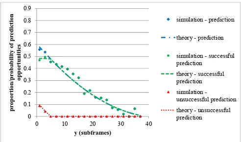
Fig. 6(a), 6(b) and 6(c) illustrate , and
calculated as an output of the simulation versus the corresponding theoretical models of Section IV.B and Section IV.C for one way predictive uplink resource allocation as a
function of the parameter for 40 subframes. Fig. 6(a)
represents the case of 5 subframes, Fig. 6(b) the case of 10 subframes and Fig. 6(c) the case of 20 subframes. It is clear that the simulation results and theoretical models match quite closely. In addition, the simulation results exhibit some traits predicted by the theoretical models. For example,
for , , or equivalently,
0.
As the value of increases for a given value of , the
proportion of predictions increases, primarily
because the eligibility criterion for a prediction is more likely to be satisfied. However, the proportion of unsuccessful predictions resulting in resource wastage also increases because the predictive resource allocation targeting the device is more likely to occur before the disturbance has reached it, at which time the device has no data to send. This explains why the proportion of successful predictions
[image:9.595.37.288.277.563.2]Fig. 6(a): Prediction Probabilities for One Way Prediction ( 40
subframes and 5 subframes)
Fig. 6(b): Prediction Probabilities for One Way Prediction ( 40
subframes and 10 subframes)
Fig. 6(c): Prediction Probabilities for One Way Prediction ( 40
subframes and 20 subframes)
Fig. 7(a) illustrates the resource usage probability of the PUCCH due to SRs (either as a result of no prediction or an unsuccessful prediction) and Fig. 7(b) illustrates the wastage probability of the PUSCH (and by extension the PDCCH) due to unsuccessful predictions calculated as an output of the simulation versus the corresponding theoretical models of Section IV.C and Section IV.D as a function of the parameter
for 40 subframes and various values of . Again the
simulation results and theoretical models show very good agreement. We see in particular from Fig. 7(a) that the proportion of data transfers requiring an SR to be sent on the PUCCH (i.e. following the normal reactive LTE uplink
resource allocation request model) is minimised for ,
thereby minimising the use of PUCCH resources. However, the proportion of unsuccessful predictions which involve a wasted predictive uplink grant on the PDCCH and a wasted predictive resource allocation for uplink data transfer on the PUSCH increases with decreasing for as seen in Fig. 7(b).
Fig. 7(a): PUCCH Resource Usage Due to SRs for One Way Prediction ( 40 subframes and various values of )
Fig. 7(b): PUSCH Resource Wastage Due to Unsuccessful Predictions for One Way Prediction ( 40 subframes and various
values of )
Fig. 7(a) and Fig. 7(b) imply that the optimum value of from a resource usage and wastage perspective is since there are no wasted PDCCH/PUSCH resources and the utilisation of the PUCCH for sending SRs is close to its minimum value.
Fig. 8 illustrates the mean uplink delay for all prediction opportunities (i.e. whether the packets were ultimately transferred as a result of predictive resource allocation or not) calculated as an output of the simulation versus the corresponding theoretical models of Section IV.E and Section IV.F for a lightly loaded system as a function of the parameter
0 0.1 0.2 0.3 0.4 0.5 0.6 0.7 0.8 0.9
0 10 20 30 40
p rop or tion/ p ro bab ility of pr ed ic tion opp o rt u n ities y (subframes)
simulation - prediction theory - prediction simulation - successful prediction theory - successful prediction simulation -unsuccessful prediction theory - unsuccessful prediction 0 0.1 0.2 0.3 0.4 0.5 0.6 0.7 0.8 0.9
0 10 20 30 40
p rop or tion/ p ro bab ility of pr ed ic tion opp o rt u n ities y (subframes)
simulation - prediction theory - prediction simulation - successful prediction theory - successful prediction simulation -unsuccessful prediction theory - unsuccessful prediction 0 0.1 0.2 0.3 0.4 0.5 0.6 0.7 0.8 0.9 1
0 10 20 30 40
p ropo rt io n /pr o babilit y o f pr edict ion o p p o rt un it ies y (subframes)
simulation - PUCCH resource used, τ=5 theory - PUCCH resource used, τ=5 simulation - PUCCH resource used, τ=10 theory - PUCCH resource used, τ=10 simulation - PUCCH resource used, τ=20 theory - PUCCH resource used, τ=20
0 0.1 0.2 0.3 0.4 0.5 0.6 0.7 0.8 0.9 1
0 10 20 30 40
p ropo rt io n /pr o babilit y o f pr edict ion o p p o rt un it ies y (subframes)
simulation - PUSCH resource wasted, τ=5 theory - PUSCH resource wasted, τ=5
[image:10.595.43.289.86.231.2] [image:10.595.308.553.226.371.2] [image:10.595.44.290.274.420.2] [image:10.595.310.554.418.565.2] [image:10.595.44.291.469.612.2]for 40 subframes and various values of . With reference to Fig. 1 and Section IV.E, the expected uplink delay when predictive resource allocation is not employed is 1
[image:11.595.306.553.212.361.2]/2 subframes (for the SR delay) plus 1 subframe (for the uplink grant from the eNodeB) plus 4.5 subframes (for the expected delay of 0.5 subframes that the data is available in the buffer before an SR can possibly be sent and the fixed grant to data transfer delay of 4 subframes). For 40 subframes, this corresponds to an expected delay of 26 subframes or ms, which is exactly the value that the simulated and theoretical models converge to as approaches (and therefore as the probability of a prediction reduces to zero) in Fig. 8. Note that this value is also the minimum mean delay that can be achieved by any non-predictive resource allocation algorithm e.g. Earliest Deadline First (EDF) [23].
Fig. 8: Mean Uplink Delay for One Way Prediction ( 40
subframes and various values of )
The one way prediction algorithm, while extremely simple and requiring very little computation in the eNodeB, affords maximum savings of over 25% in mean uplink delay in this example relative to the minimum mean delay possible with a non-predictive resource allocation algorithm. It can be seen that operating at results in a significant saving in mean uplink delay in Fig. 8 while optimising the usage and wastage of resources in Fig. 7(a) and Fig. 7(b). Another interesting observation is that, for a given value of the parameter , the mean uplink delay exhibits only a weak dependence on the value of , with the maximum disparity occurring at
approximately /2.
Fig. 9 illustrates the mean uplink delay for all prediction opportunities calculated as an output of the simulation versus the corresponding theoretical models of Section IV.E and Section IV.F for a lightly loaded system as a function of the parameter for 10 subframes and various realistic values of . As before, the expected uplink delay when predictive
resource allocation is not employed is 1 /2 1
where 4.5; this equates to 16ms for 20 subframes,
26ms for 40 subframes and 46ms for 80 subframes.
These are exactly the values that the simulated and theoretical models converge to as approaches (and therefore as the probability of a prediction reduces to zero) in Fig. 9. These values also represent the minimum mean delay that can be achieved by any non-predictive resource allocation algorithm.
Again it can be seen that operating at results in a
significant saving in mean uplink delay in Fig. 9 for any value of while optimising the usage and wastage of resources (see Fig. 7(a) and Fig. 7(b) for the case of 40 subframes). In proportionate terms, the maximum reduction in mean uplink
delay increases as increases. For example, for 20
subframes, the maximum reduction in mean uplink delay is approximately 22% (down from 16ms to 12.5ms), and for 80 subframes, the maximum reduction in mean uplink delay is approximately 30% (down from 46ms to 32ms).
Fig. 9: Mean Uplink Delay for One Way Prediction ( 10
subframes and various values of )
V.UTILITY OF MODELS
We have already noted that the mathematical models for predictive resource allocation developed in this paper can be employed offline or online by network operators to configure the aggressiveness of a prediction strategy as a compromise between reduced latency and wasted resources. We consider the more interesting online option here in which the eNodeB estimates certain characteristics of the group traffic profile in real time in order to modify the algorithm parameters dynamically for optimum performance.
For example, as discussed in Section IV.G, assume that the desired operating configuration is in order to reduce the mean uplink latency as much as possible using predictive resource allocation without wasting resources, and assume is initially unknown. The eNodeB chooses an initial value
. If unsuccessful predictive resource allocations are
experienced, it is clear from Eq. (10) that and
therefore the value of can be increased in real time while predictions are still taking place in order to reduce wasted PDCCH/PUSCH resources. Conversely, if all predictive resource allocations are successful, it is clear that
and therefore the value of can be decreased in real time while predictions are still taking place in order to reduce mean uplink latency.
Other optimisation algorithms based upon the mathematical models are possible in which the value of is estimated directly rather than iteratively. For example, if the probability of a prediction can be estimated in real time as predictions are occurring, Eq. (8) can be employed with and the prevailing
18 19 20 21 22 23 24 25 26 27 28
0 10 20 30 40
m
ean
u
p
lin
k
delay (m
s)
for
pr
ed
ict
ion
o
p
po
rt
un
it
ie
s
y (subframes)
simulation τ=5 theory τ=5 simulation τ=10 theory τ=10 simulation τ=20 theory τ=20 best case for non-predictive scheduler
0 5 10 15 20 25 30 35 40 45 50
0 20 40 60 80
m
ean uplink
delay
(
m
s)
fo
r
pr
edict
ion
oppo
rt
u
n
it
ies
y (subframes)
[image:11.595.45.290.260.407.2]value of to provide an estimate of . The value of can then be set to the estimate of for future predictions.
VI.ADDITIONAL INSIGHTS
In this section, we provide additional insights into the one way predictive uplink resource allocation algorithm, focusing on practical aspects.
A.Random
Except in rare cases involving a carefully planned sensor deployment, the inter-sensor propagation time of the disturbance is unlikely to be a fixed value. Fig. 10 illustrates
, and calculated as simulation
outputs when is distributed according to uniform and
exponential distributions with 10 subframes versus the
corresponding theoretical models of Section IV.B and Section IV.C for constant 10 subframes. In the case of the uniform
distribution, ~ 0,20 , and in the case of the
exponential distribution, ~ 0.1 where the rate
[image:12.595.307.553.167.330.2]parameter 0.1 sensors/subframe.
Fig. 10: Prediction Probabilities for One Way Prediction and Random ( 40 subframes)
It is clear from Fig.10 that the theoretical model for the probability of a prediction with constant provides a good fit even when is random. However, the theoretical models for a successful and unsuccessful prediction are less appropriate. This is expected, because for constant , a prediction can only
be unsuccessful when as discussed in Section IV.C, but
with random for which an arbitrary value of can by definition be greater than , the range of possible values of
for which unsuccessful predictions can occur is increased. In
particular, we note that for ~ 0,20 , the probability
of an unsuccessful prediction is greater than zero for 0
20 subframes, whereas for ~ 0.1 in which the
maximum value of is not constrained, the probability of an
unsuccessful prediction is greater than zero for 0 40
subframes given that 40 subframes.
Fig. 11 illustrates the mean uplink delay for all prediction opportunities calculated as an output of the simulation when is distributed according to the same uniform and exponential distributions as for Fig. 10 versus the corresponding theoretical
models of Section IV.E and Section IV.F for constant 10
[image:12.595.44.290.325.470.2]subframes. It can be seen that the mean delay is increased marginally for random , particularly for small and intermediate values of . This is again expected due to the fact that the probability of a/an successful/unsuccessful prediction changes when is random compared to the case when is constant.
Fig. 11: Mean Uplink Delay for One Way Prediction and Random ( 40 subframes)
B.Effect of Background Traffic
The effect of background traffic on prediction performance is clearly of interest since event based M2M traffic will generally coexist with other traffic types in a real deployment. We employed 100 background devices in the simulation with exponential packet inter-arrivals of a given rate to load the system. The background and event based M2M sensor traffic were given equal priority by the eNodeB scheduler. For a background traffic rate of 50 packets per second per background device, the radio network is close to fully saturated with PDCCH utilization of 97.35% and PUSCH utilization of
99.78%. Fig. 12 illustrates , and
calculated as simulation outputs for different background traffic rates versus the corresponding theoretical models of Section IV.B and Section IV.C for constant 10 subframes. Not all combinations are shown for clarity.
Fig. 12 demonstrates that the probability of a prediction is not significantly affected by the presence of background traffic. This is expected because, as explained in Section IV.A, the decision to perform a prediction depends only upon the scheduled timing of SR opportunities which is fixed for any one sensor. However, as the background traffic increases, the probability of a successful prediction actually increases (or alternatively the probability of an unsuccessful prediction decreases). This may initially seem counter intuitive, but one must remember that a prediction targeting a sensor is unsuccessful if it occurs prior to the disturbance reaching the sensor as explained in Section IV.C. Increasing the background traffic generally increases the delay in sending the predictive uplink grant which in turn increases the probability that the disturbance will have arrived at the sensor prior to the prediction. We also note that the background traffic has to 0
0.1 0.2 0.3 0.4 0.5 0.6 0.7
0 10 20 30 40
pr
op
or
ti
on/
p
ro
babi
li
ty
of
pr
ed
ic
ti
o
n
op
por
tuni
ti
es
y (subframes)
simulation - prediction, τ~uniform(0,20) simulation - prediction, τ~exponential(0.1) theory - prediction, τ=10
simulation - successful prediction, τ~uniform(0,20) simulation - successful prediction, τ~exponential(0.1) theory - successful prediction, τ=10
simulation - unsuccessful prediction, τ~uniform(0,20) simulation - unsuccessful prediction, τ~exponential(0.1) theory - unsuccessful prediction, τ=10
0 5 10 15 20 25 30
0 10 20 30 40
m
ea
n
up
li
nk
de
la
y
(
m
s)
fo
r p
re
d
ic
ti
o
n
o
ppo
rt
u
n
it
ie
s
y (subframes)
simulation,
τ~uniform(0,20) simulation,
reach a certain level to have any significant effect on the prediction performance. For example, for a background traffic rate of 25 packets per second per background device, there is no significant difference in prediction performance versus no background traffic. Again this is expected because scheduling delays only occur when there is too much traffic to be serviced by the available instantaneous PDCCH and PUSCH resources.
[image:13.595.305.552.199.365.2]Fig. 12: Prediction Probabilities for One Way Prediction with Background Traffic (σ=40 subframes and τ=10 subframes)
Fig. 13 illustrates the mean uplink delay for all prediction opportunities calculated as an output of the simulation for different background traffic rates versus the corresponding theoretical models of Section IV.E and Section IV.F for
constant 10 subframes. It can be seen that one way
[image:13.595.43.291.486.653.2]prediction can still be effective in reducing mean uplink delay even in the presence of a high load from background traffic and that the background traffic must surpass a certain level to have any significant effect on the delay performance of predictions.
Fig. 13: Mean Uplink Delay for One Way Prediction with Background Traffic (σ=40 subframes and τ=10 subframes)
C.Comparison with Other Prediction Algorithms
Although the primary focus of this paper is on the one way predictive uplink resource allocation algorithm because it affords a tractable mathematical analysis, it is useful to
compare the performance of this algorithm with more complex algorithms via simulation. Fig. 14 illustrates the mean uplink delay of all packets calculated as an output of the simulation for one way prediction, two way prediction and two way prediction with chaining [12]. It can be seen that the two way prediction algorithm affords only a small benefit over the one way prediction algorithm in terms of reduced delay, but the addition of the chaining feature results in significantly improved performance.
Fig. 14: Mean Delay of All Uplink Packets for Different Prediction Algorithms ( 40 subframes and 10 subframes)
VII.CONCLUSIONS
In this paper, we have introduced a new predictive resource allocation algorithm in the LTE uplink for event based M2M applications, the so called one way algorithm. This algorithm can reduce the mean uplink delay significantly below the minimum possible for a non-predictive resource allocation algorithm by exploiting correlation of the traffic patterns of M2M devices in a group. Mathematical models relating to the probability of a prediction, the probability of a successful prediction, the probability of an unsuccessful prediction, resource usage/wastage probabilities and expected uplink latency have been developed. These models have been validated via a bespoke LTE based simulation model using the OPNET platform. The models can be used both offline and online by network operators to configure the aggressiveness of a prediction strategy as a compromise between reduced latency and wasted resources. We briefly outlined how the mathematical models may be employed online by the eNodeB to optimise the operation of the prediction algorithm in real time via iteration or direct estimation.
Further work includes generalising the models to be applicable to scattered 2D and 3D device topologies using multi-directional prediction. We also plan to develop and analyse more complex predictive resource allocation algorithms and in particular introduce the effect of prediction chaining into the models in which a successful predictive allocation can itself be the trigger for another prediction.
0 0.1 0.2 0.3 0.4 0.5 0.6 0.7
0 5 10 15 20 25 30 35 40
p
roportion
/pr
o
babi
lity of
p
rediction
op
portun
ities
y (subframes)
simulation - prediction, 50pps per BG device
theory - prediction, zero BG traffic
simulation - successful prediction, 50pps per BG device theory - successful prediction, zero BG traffic
simulation - unsuccessful prediction, 25pps per BG device simulation - unsuccessful prediction, 37.5pps per BG device simulation - unsuccessful prediction, 50pps per BG device theory - unsuccessful prediction, zero BG traffic
0 5 10 15 20 25 30 35 40
0 10 20 30 40
m
ea
n
up
li
nk
de
la
y
(
m
s)
fo
r p
re
d
ic
ti
o
n
o
ppo
rt
u
n
it
ie
s
y (subframes)
simulation, 25pps per BG device
simulation, 37.5pps per BG device
simulation, 50pps per BG device
theory, zero BG traffic
0 5 10 15 20 25 30
0 10 20 30 40
m
ean
d
elay (
m
s)
for
al
l
up
li
n
k
p
a
ck
et
s
y (subframes)
One way prediction
Two way prediction
ACKNOWLEDGMENT
This work has been supported by Ausgrid and the Australian Research Council (ARC).
REFERENCES
[1] 3GPP TR 25.913 V8.0.0 (2008-12), “Requirements for Evolved UTRA (E-UTRA) and Evolved UTRAN (E-UTRAN)”, Rel. 8
[2] Dajie Jiang, Haiming Wang, Malkamaki, E., Tuomaala, E.,
“Principle and Performance of Semi-Persistent Scheduling for VoIP in LTE System”, Wireless Communications, Networking and Mobile Computing, 2007. WiCom 2007. International Conference on, pp. 2861-2864, 21-25 Sept. 2007
[3] Jing Han; Haiming Wang, “Principle and Performance of TTI Bundling For VoIP in LTE FDD Mode”, Wireless Communications and Networking Conference, 2009. WCNC 2009. pp.1-6, 5-8 April 2009
[4] Jason Brown, Jamil Y. Khan, “Key performance aspects of an LTE FDD based Smart Grid communications network”, Elsevier Computer Communications, Volume 36, Issue 5, 1 March 2013, Pages 551-561
[5] Kan Zheng; Fanglong Hu; Wenbo Wang; Wei Xiang; Dohler,
M., “Radio resource allocation in LTE-advanced cellular networks with M2M communications”, Communications Magazine, IEEE , vol.50, no.7, pp.184-192, July 2012
[6] Gotsis, A.G.; Lioumpas, A.S.; Alexiou, A., “M2M Scheduling over LTE: Challenges and New Perspectives”, Vehicular Technology Magazine, IEEE , vol.7, no.3, pp.34-39, Sept. 2012 [7] 3GPP TS 22.368 V10.5.0 (2011-07), “Service requirements for
Machine-Type Communications (MTC); Stage 1”, Release 10. [8] Shafiq, M.Z.; Lusheng Ji; Liu, A.X.; Pang, J.; Jia Wang,
"Large-Scale Measurement and Characterization of Cellular Machine-to-Machine Traffic," Networking, IEEE/ACM Transactions on , vol.21, no.6, pp.1960-1973, Dec. 2013
[9] Jason Brown and Jamil Y. Khan, “Performance Comparison of LTE FDD and TDD Based Smart Grid Communications Networks for Uplink Biased Traffic”, Smart Grid Communications (SmartGridComm), 2012 IEEE International Conference on, 5-8 Nov. 2012
[10]Patel A., Aparicio J., Tas N., Loiacono M., Rosca J., “Assessing Communications Technology Options for Smart Grid Applications”, Smart Grid Communications (SmartGridComm), 2011 IEEE International Conference on, 2011, pp. 126-131
[11]Rongduo Liu, Wei Wu, Hao Zhu and Dacheng Yang,
“M2M-Oriented QoS Categorization in Cellular Network”, Wireless Communications, Networking and Mobile Computing (WiCOM), 2011 7th International Conference on, pp.1-5, 23-25 Sept. 2011
[12]Jason Brown and Jamil Y. Khan, “Predictive Resource
Allocation in the LTE Uplink for Event Based M2M Applications”, IEEE International Conference on Communications (ICC) 2013, Beyond LTE-A Workshop, 9 June 2013
[13]Teixeira, M.A.; Guardieiro, P.R.; "A predictive scheduling algorithm for the uplink traffic in IEEE 802.16 networks," Advanced Communication Technology (ICACT), 2010 The 12th International Conference on , vol.1, no., pp.651-656, 7-10 Feb. 2010
[14]Tadrous, J.; Eryilmaz, A.; El Gamal, H., "Proactive Resource Allocation: Harnessing the Diversity and Multicast Gains", Information Theory, IEEE Transactions on, vol.59, no.8, pp.4833-4854, Aug. 2013
[15]El Gamal, H., Tadrous, J. and Eryilmaz, A.; "Proactive resource allocation: Turning predictable behavior into spectral gain,"
Communication, Control, and Computing (Allerton), 2010 48th Annual Allerton Conference on, Sept. 29 2010-Oct. 1 2010
[16]Tadrous, J., Eryilmaz, A., El Gamal, H. and Nafie, M.;
“Proactive resource allocation in cognitive networks”, Signals, Systems and Computers (ASILOMAR), 2011 Conference Record of the Forty Fifth Asilomar Conference on, pp.1425-1429, 6-9 Nov. 2011
[17]Asheralieva, A., Khan, J.Y., Mahata, K. and Eng Hwee Ong, “A predictive network resource allocation technique for cognitive wireless networks”, Signal Processing and Communication Systems (ICSPCS), 2010 4th International Conference on, pp.1-9, 13-15 Dec. 2010
[18]3GPP TS 36.331 V10.12.0 (2014-01), “Evolved Universal
Terrestrial Radio Access (E-UTRA); Radio Resource Control (RRC); Protocol specification”, Release 10.
[19]3GPP TS 36.321 V10.10.0 (2014-01), “Evolved Universal
Terrestrial Radio Access (E-UTRA); Medium Access Control (MAC) protocol specification”, Release 10
[20]3GPP TS 36.213 V10.12.0 (2014-03), “Evolved Universal
Terrestrial Radio Access (E-UTRA); Physical layer procedures”, Release 10
[21]3GPP TS 36.101 V10.13.0 (2014-01), “Evolved Universal
Terrestrial Radio Access (E-UTRA); User Equipment (UE) radio transmission and reception", Release 10
[22]V. Erceg et al., “An empirically based path loss model for wireless channels in suburban environments”, IEEE JSAC, vol.17, no.7, July 1999, pp. 1205-1222.
[23]Sivaraman, V.; Chiussi, F., "End-to-end statistical delay guarantees using earliest deadline first (EDF) packet scheduling," Global Telecommunications Conference, 1999. GLOBECOM '99 , vol.2, no., pp.1307,1312 vol.2, 1999
Jason Brown received his BEng and Ph.D. from the University of Manchester Institute of Science and Technology (UMIST) in 1990 and 1994 respectively. He has worked in R&D and operational roles for Vodafone, AT&T and LG Electronics. In 2011, he joined the University of Newcastle in Australia researching smart grid and M2M communications technologies. His main research interest areas are 4G and 5G wireless networks, smart grid communications, M2M communications and wireless sensor networks.