The SPIDER CMB Polarimeter

The S

CMB Polarimeter

Thesis by Amy R. Trangsrud

In Partial Fulfillment of the Requirements for the Degree of

Doctor of Philosophy

California Institute of Technology Pasadena, California

2012

Acknowledgements

My journey here began one September day, walking into Andrew Lange’s office in the basement of West Bridge, excited and nervous. In a moment he saw me, took me in, welcomed me, and set me at ease. Then we were off like a whirlwind. We walked briskly over to the high bay, whereBICEPwas nearing deployment. Andrew sent me up on a ladder to take in the technology, while he told me about B-modes,Spider, andBICEP2, his eyes alight with excitement. He oozed curiosity, ingenuity, and enthusiasm. Back in Bridge, he toured me through the White Dewar lab, where Chao-Lin Kuo was beam mapping. I remember Andrew saying, this could be you in a couple years. Sure enough, it was.

Andrew was exceptional in his ability to advise, understand, and nurture his students. When I sat down with him, he would immediately focus in on my situation and perspective, and on how he could best aid me in moving forward. He saw things in context, and gave science a sense of humanity. Andrew understood that the relationship between a PhD student and an advisor is a special one; one that plants a seed that shapes the student over a lifetime. So it will be for me. I am grateful and honored that Andrew shared his spirit with me, and I will carry and treasure his mentorship and example. Thank you Andrew.

When we lost Andrew, our Obscos team grew even stronger as a family. Kathy Deniston, Sunil Golwala, and Jamie Bock, while handling their own grief, opened their wings like protective parents, and swept everyone under. They were heros in a dark time. Simply put, we would not have a group without Kathy. She and Barbara Wertz are simultaneously the glue that holds everything together and the grease that keeps everything moving. To this day, I am not sure how Kathy does it all.

concepts clearly and to derive relevant results on a moment’s notice.

There is no one in this group with whom I have worked as closely and over as many years as Jamie. Spider is made compelling by its detector technology more than anything else. Jamie is the core of the detector development effort, and therefore at the root of everything that we do. After four years of Thursday detector meetings, I sincerely hope that a bit of Jamie’s deep understanding and intuition have rubbed off on me. I appreciate all that I have learned from him not only about the devices themselves, but about the process of developing new technology, patiently, methodically, and creatively.

I have had a number of mentors over my years here, and I appreciate each and every one of them for mentoring me, and showing me their style of science. Matt Kenyon at JPL showed me how to fly by the seat of my pants and get a lot done. Bill Jones had a way of making any task feel fun and valuable. Chao-Lin Kuo showed me how to manage experiments from start to end, and operate my own cryogenic test bed. Jeff Filippini and Marc Runyan mentored me in receiver characterization, and provided opportunities for me to take important roles in our team. There are many others. I would like to thank all of my colleagues and collaborators here at Caltech/JPL, and around the world.

Caltech is a community, and my memories of this place will extend well beyond the walls of the astronomy building. While enrolled here I met the love of my life, was sexually harassed by a janitor, was awarded a fellowship, had a life-changing surgery, lost my advisor, and got married. My friends have been with me through it all, and made this journey possible. You all know who you are. Thank you!

There is no easy way to put into words the debt I owe to my Mom and Dad for their love, support, sacrifices, patience and just plain hard work in helping me to grow into the person that I am, and in filling my life with an incredible abundance of opportunities.

The S

PIDER

Collaboration

California Institute of Technology J. P. Filippini, S. Golwala, V. V. Hristov, P. V. Mason, T. A. Morford, M. C. Runyan, M. A. Schenker, A. R. Trangsrud, R. S. Tucker Cardiff University P. A. R. Ade, C. Tucker

Case Western Reserve University R. Bihary, S. Bryan, T. E. Montroy, J. E. Ruhl Imperial College C. N. Clark, C. R. Contaldi, D. T. O’Dea

JPL J. J. Bock, J. A. Bonetti, B. P. Crill, O. Dor´e, W. Holmes, A. D. Turner Kavli Institute for Cosmology, University of Cambridge C. J. MacTavish NIST G. Hilton, K. Irwin, C. Reintsema

Princeton University H. C. Chiang, A. A. Fraisse, J. E. Gudmundsson, W. C. Jones, A. S. Rahlin

Stanford University C. L. Kuo

University of Toronto S. J. Benton, M. Farhang, L. M. Fissel, N. N. Gandilo, C. B. Netterfield, J. D. Soler, J. A. Shariff, J. R. Bond

Abstract

Spider is a balloon-borne millimeter-wave telescope designed to study the polarization of the Cosmic Microwave Background (CMB).Spiderwill map 10% of the full sky with degree-scale beams to search for the distinctive inflationary gravitational wave signal on angular scales between 1◦ and 10◦, thereby probing the energy scale of inflation. In its first flight,

Contents

Acknowledgements iii

The SPIDER Collaboration v

Abstract vi

1 Introduction 1

1.1 The Beginning of Physical Cosmology . . . 1

1.2 Discovery of the Cosmic Microwave Background . . . 4

1.3 CMB Statistics . . . 5

1.4 Inflation Theory . . . 9

1.5 CMB Temperature Anisotropies . . . 12

1.6 CMB Polarizing Mechanisms . . . 13

1.7 Polarized Foregrounds . . . 19

2 The SPIDERBalloon-Borne CMB Polarization Experiment 22 2.1 Collaboration . . . 23

2.2 Frequency Coverage . . . 23

2.3 Sky Coverage . . . 26

2.4 Ballooning . . . 26

2.5 Cryogenics . . . 30

2.6 Optics . . . 33

2.7 Half-Wave Plates . . . 37

2.8 Magnetic Shielding . . . 39

3 Detectors and Readout 42

3.1 Bolometric Technology Development . . . 42

3.2 SPIDERDetector Architecture . . . 45

3.3 Fabrication Process . . . 49

3.4 TES Bolometer Basics . . . 52

3.5 Readout . . . 58

4 Receiver Performance 61 4.1 Beam Profiles . . . 61

4.2 Frequency Band Definition . . . 71

4.3 Polarization Efficiency . . . 79

4.4 Efficiency of Optical Response . . . 80

4.5 Internal Optical Loading of Devices . . . 86

4.6 Bolometer Properties . . . 90

4.7 Noise Performance . . . 94

4.8 Temperature Stability . . . 100

4.9 Magnetic Field Response . . . 101

4.10 Summary and Recommendations for Future Work . . . 102

A Definitions and Methods 107 A.1 Optical Efficiency . . . 107

A.2 Alternative Methods for Calculating Internal Loading . . . 109

B Measured Detector Parameters 112

List of Figures

1.1 Example of a CMB temperature and polarization map (from B2K) . . . 7

1.2 Illustration of E- and B-mode polarization patterns . . . 8

1.3 Definition of coordinate system for Thomson scattering calculation . . . 14

1.4 Measurements to date of EE and BB power spectra . . . 21

2.1 Spider bands and atmospheric emission model . . . 25

2.2 TheSpider observing region . . . 26

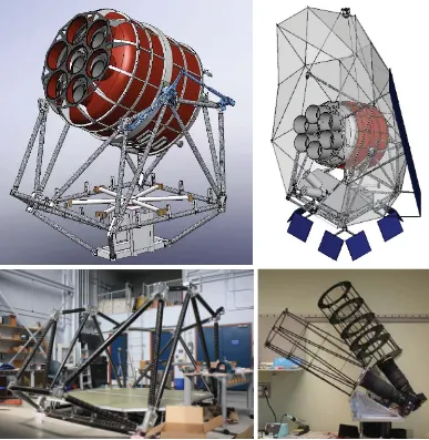
2.3 TheSpider gondola (drawings and photos) . . . 29

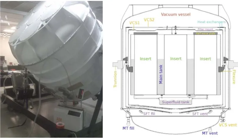
2.4 TheSpider flight cryostat (photo and cross-sectional drawing) . . . 31

2.5 An assembled focal plane unit and a3He adsorption fridge (photos) . . . 32

2.6 Modular telescope insert bays in the flight cryostat (photos) . . . 34

2.7 A telescope insert (photo and cross-sectional drawing) . . . 34

2.8 A half-wave plate assembly (photos) . . . 37

2.9 Diagram showing rotation of polarization by a half-wave plate . . . 38

2.10 Sensitivity of Spider bands to polarized dust . . . 41

3.1 A spider-web bolometer and a polarization sensitive bolometer (photos) . . . 43

3.2 New technologies have enabled a large increase in detector counts . . . 44

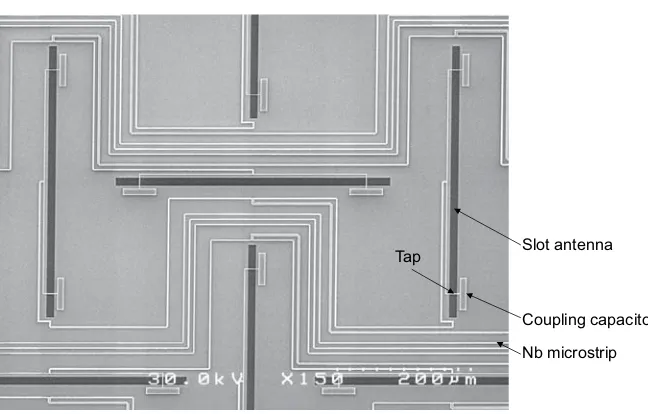
3.3 A Spiderdetector plate and a single pixel with components labeled (photos) 45 3.4 A portion of a slot antenna array (SEM micrograph) . . . 47

3.5 An LC microstrip filter (SEM micrograph) . . . 47

3.6 Silicon nitride legs thermally isolate each bolometer island (optical micrograph) 48 3.7 A bolometer island with substructures labeled (optical micrograph) . . . 48

3.8 I-V curve showing both the Ti TES and Al TES transitions . . . 48

3.9 A T-junction in an antenna microstrip summing tree (SEM micrograph) . . . 51

3.10 Cross-sectional schematic of the layered construction of the dual-TES . . . . 51

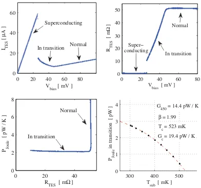
3.12 I-V, R-V and P-V curves, and method to measure leg thermal conductance . 56

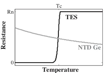
3.13 A comparison of TES and NTD Ge thermistor response functions . . . 57

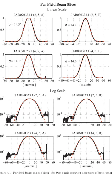
4.1 Far field beam slices (linear and log scale) . . . 63

4.2 Far field beam differences for a single pixel A/B polarization pair . . . 64

4.3 Near field beam maps showing the effects of beam steer . . . 66

4.4 Antenna far field beam maps (no telescope) for an A/B polarization pair . . 69

4.5 Primary antenna sidelobes (terminated inside telescope) . . . 70

4.6 Beam maps showing uniform vs Gaussian-tapered feed . . . 71

4.7 Measured flightlike 148 GHz passband and old-style 145 GHz passband . . . 73

4.8 Histogram and map of measured band centers on a 148 GHz tile . . . 74

4.9 Spectra and differenced spectra for 148 GHz A/B polarization pairs . . . 75

4.10 Convolution of the atmospheric model with the measured 148 GHz passband 76 4.11 Spectral model for 93 GHz band . . . 77

4.12 Convolution of the atmospheric model with the 93 GHz passband model . . . 78

4.13 Measurement of cross-polarization response . . . 80

4.14 The cold load cryostat (photos) . . . 81

4.15 Setup for White Dewar single pixel optical efficiency measurement (photos) . 82 4.16 Histogram of measured signal attenuation by microstrip summing tree . . . . 84

4.17 Basic method for measuring internal loading . . . 87

4.18 Measured internal loading is strongly correlated with measured sky response 88 4.19 R-V curves illustrating the impact of shared TES bias . . . 92

4.20 Example of measured noise power spectral density . . . 95

4.21 Measured noise depends on TES bias point . . . 96

4.22 Example of measured noise equivalent current, power, and temperature . . . 97

4.23 Rough estimator for noise penalty due to shared TES bias . . . 98

4.24 Comparison of dark and active devices showing the addition of photon noise 99 A.1 Optical response measurements are used to normalize device spectra . . . 108

List of Tables

2.1 Responsibilities of Spidercollaborating institutions . . . 23

2.2 Planned frequency distribution of focal plane units for first and second flights 24 4.1 Model of loss mechanisms for the 148 GHz band . . . 83

4.2 Projected optical loading on a single-polarization 148 GHz device . . . 89

4.3 Measured uniformity of fabricated device parameters . . . 93

Chapter 1

Introduction

Today we are able to make precise statements about the age, composition and evolution of the universe, though the field of physical cosmology was born only a century ago (§1.1). In 1965, the discovery of the Cosmic Microwave Background (CMB,§1.2), relic radiation from the early universe, identified a rich source of information that has enabled many advances in cosmology. The statistical properties of the CMB (§1.3) contain valuable clues about the makeup of the universe at the time of decoupling, only 400,000 years after the Big Bang. The standard model for the evolution of the universe includes a brief exponential inflation of space in the first fraction of a second after the Big Bang (§1.4). Measurements of the temperature anisotropies of the CMB support the inflationary paradigm and have tightly constrained many of the parameters of the standard model (§1.5). The CMB is polarized by several mechanisms (§1.6). Polarized galactic emission (§1.7) acts as a foreground to the CMB signal, distinguishable by its unique spectral signature. Gravitational waves predicted by inflationary theories generate a faint but distinctive CMB polarization pattern. A detection of this polarization signature would provide very strong evidence supporting the theory of inflation and probe the epoch of inflation itself.

1.1

The Beginning of Physical Cosmology

Bringing Together Space and Time

Modern physical cosmology theory has its roots in Albert Einstein’s general theory of rel-ativity, first published in 1915. General relativity is a generalization of special relrel-ativity, folding the three dimensions of space and one dimension of time into a four-dimensional space-time. Gravity falls out of the theory as a natural geometrical consequence. Einstein’s paradigm was elegant and testable, and carried cosmology into the realm of true science.

General relativity explained the discrepancy between previous calculations based on Newtonian gravity and the measured precession of the perihelion of Mercury. In 1919 Sir Arthur Eddington and his collaborators mapped stars positioned near the Sun during a total solar eclipse. General relativity predicts the bending of light due to the curvature of space time around massive objects (here, the Sun). The measured apparent locations of the stars were offset in accordance with the predictions of general relativity [41]. For the past century, general relatively has successfully stood up to increasingly precise measurements of its various predictions, including the gravitational redshift of light, gravitational lensing, and time dilation. For example, the Cassini project announced in 2003 that the frequency shift of radio signals sent between the spacecraft and Earth, due to the gravitational well of the Sun, agreed with the predictions of general relativity to 0.002% [15].

Seeing Beyond the Milky Way

In the 1920s Edwin Hubble began using the Hooker telescope on Mount Wilson just north of Pasadena, California, then the biggest telescope in the world. Applying Leavitt’s period-luminosity relationship to Cepheids that he observed in several spiral nebulae, he made the first demonstration of objects definitely outside of our galaxy [62]. His announcement to the American Astronomical Society on New Years Day in 1925 expanded the known universe beyond the Milky Way and ushered in a new era in cosmology.

In the early 1910s, Vesto Slipher examined the spectroscopic features of spiral galax-ies [111]. He was surprised to find that the galaxgalax-ies were moving at hundreds of kilometers per second relative to earth (about 25 times the average stellar velocity, he noted). Slipher’s work demonstrated that spectroscopy was a valuable tool for measuring the large radial ve-locities of galaxies using the Doppler shift. Slipher reported the veve-locities of fifteen galaxies. All but three were receding.

Big Bang Controversy

In the early 1920s Alexander Friedmann showed that general relativity does not generically predict the static universe put forth by Einstein [46, 47]. In general, the curvature of the universe can be time dependent and the universe may expand or contract. Friedmann’s equations and conclusions were independently derived by Georges Lemaˆıtre in the late 1920s [81, 82]. Lemaˆıtre described a homogenous universe of constant mass and increasing radius. This accounted for the observed preponderance of galaxies receding from our own. In 1929, Hubble demonstrated a positive linear relation between the distance to nearby galaxies (measured using Cepheids) and their radial velocities (measured spectroscopically using redshift) [61]. The combination of this relation (“Hubble’s law”) with the Cosmolog-ical Principle (an assumption of homogeneity and isotropy on large scales) implies that the universe is expanding.

The debate between Big Bang theory and Steady State theory was a central dialog in cosmology until the 1965 publication of the discovery of the Cosmic Microwave Background, relic radiation from the hot Big Bang.

1.2

Discovery of the Cosmic Microwave Background

Astro-physical Journal Letters published, side-by-side, letters from the Princeton group [37] and the Bell Labs group [100]. The following year Roll and Wilkinson at Princeton, measuring at a wavelength of 3.2 cm, published flux results consistent with blackbody radiation at 3.0±0.5 K [106].

TheCOBEsatellite, launched in 1989, carried several experiments to study the CMB. The FIRAS experiment measured its spectrum over a broad frequency range. The data mapped out the curve of a black body with temperature 2.725±0.002 K [92]. TheCOBE anisotropy experiment, called DMR, found the CMB to be greatly isotropic [113]. Tem-perature anisotropies are usually decomposed into spherical harmonics (§1.3). The dipole term is dominated by the Earth’s motion relative to the Hubble Flow and is irrelevant to cosmological anisotropy considerations. The small size of the remaining observed tempera-ture anisotropy (ΔT /T ≈10−5) excluded models that claimed that the CMB had a galactic source or random distribution of sources. This was a solid confirmation of Big Bang theory to the exclusion of Steady State theories.

1.3

CMB Statistics

The statistical properties of the CMB are a fruitful testing ground for cosmological theories. I here review the standard mathematical framework for quantifying CMB temperature and polarization statistics. Throughout this section I follow Kamionkowski et al. [68].

The Stokes Parameters

Polarization is conventionally defined in terms of the Stokes parameters. A linearly (plane) polarized electromagnetic wave has an oscillating electric field at a fixed azimuthal angle to the direction of propagation. A wave with two perpendicular components of equal amplitude that are out of phase by 90◦ is called a circularly polarized wave. For a monochromatic wave propagating along the z-axis, linear polarization can be described by

Polarization is completely quantified using the Stokes parameters ( denotes a time aver-age):

I ≡ |Ex|2+|Ey|2, (1.2a)

Q ≡ |Ex|2− |Ey|2, (1.2b)

U ≡ 2|Ex||Ey|cos (θx−θy), and (1.2c) V ≡ 2|Ex||Ey|sin (θx−θy). (1.2d)

The Stokes parameters have units of power and are additive for an incoherent superposition of waves. The parameterIrepresents the intensity of the radiation and is positive definite. It is the most commonly observed parameter, and in this case is simply proportional to the temperature of the CMB. The other three parameters quantify the polarization state, with Q = U =V = 0 for unpolarized radiation. Stokes Q and U measure linear polarization along axes rotated 45◦ with respect to one another. The parameter V quantifies circular polarization, which is expected to be zero for the CMB because, by symmetry, Thomson scattering processes can never produce any net circular polarization.

The orthogonal modes of linear polarization given by Q and U are dependent on the defined orientations of the x- and y-axes. The orientations are defined by the International Astronomical Union (IAU) convention. Taking the definitions ofQandU from Equation 1.2 and rotating the x–y plane through an angleφgives new values forQand U:

Q = Qcos(2φ) +Usin(2φ) , and (1.3a)

U = −Qsin(2φ) +Ucos(2φ) . (1.3b)

It is easy to show thatQ2+U2=Q2_+U2_{, so Q}2_+U2 _{is invariant under axis rotation.}

We can define the amplitude and orientation of the polarization:

P ≡Q2_+U2_{, and (1.4a)}

α≡1

2tan −1U

Q . (1.4b)

Figure 1.1: Example of a polarization and temperature map, from theB2Kexperiment [90].

field oscillates. Polarization maps are usually plotted as headless vectors with amplitudeP and orientation angleα(see, for example, Figure 1.1).

The Harmonic Functions

The cosmological information encoded in the CMB is in the spatial correlations of the Stokes parameters. To quantify correlations in intensity at various angular scales, we decompose the temperature anisotropy scalar field into the spherical harmonicsYlm(θ, φ),

T(θ, φ)

T0

= 1 + ∞

l=1

l

m=−l

aT_lmYlm(θ, φ). (1.5)

Polarization is described by a 2×2 symmetric and trace-free tensor field. We construct it in spherical polar coordinates as

Pab(θ, φ) = 1 2

⎛

⎝ Q(θ, φ) −U(θ, φ) sinθ

−U(θ, φ) sinθ −Q(θ, φ) sin2_θ ⎞

The polarization tensor can be decomposed into an orthonormal basis of tensor harmonics,

Pab(θ, φ)

T0 = ∞ l=2 l

m=−l

aE_lmY_lmE(θ, φ) +aB_lmY_lmB(θ, φ) , (1.7)

where the coefficients are given by

aElm =

1

T0

sinφdθdφPab(θ, φ)YlmE(θ, φ)

∗

, and (1.8a)

aB_lm = 1

T0

sinφdθdφPab(θ, φ)YlmB(θ, φ)

∗

. (1.8b)

The harmonics are

Y_lmE(θ, φ) =

2(l−2)! (l+ 2)!

⎛

⎝ Wlm(θ, φ) Xlm(θ, φ) sinθ Xlm(θ, φ) sinθ −Wlm(θ, φ) sin2θ

⎞

⎠, and (1.9a)

Y_lmB(θ, φ) =

2(l−2)! (l+ 2)!

⎛

⎝ −Xlm(θ, φ) Wlm(θ, φ) sinθ Wlm(θ, φ) sinθ Xlm(θ, φ) sin2θ

⎞

⎠, (1.9b)

with

Wlm(θ, φ) = 2

∂

∂θ2 −l(l−1)

Ylm(θ, φ), and (1.10a)

Xlm(θ, φ) =

2im sinθ

∂

∂θ −cotθ

Ylm(θ, φ). (1.10b)

The Y_lmE and Y_lmB tensor harmonics (Equations 1.9a,b) form a complete basis. Figure 1.2 shows examples of maps containing only Y_lmE harmonics or only Y_lmB harmonics. The Y_lmE harmonics are called E-modes and the Y_lmB harmonics are called B-modes, in analogy to curl-free electric (E) and divergence-free magnetic (B) fields.

Power Spectra

Assuming Gaussianity, theax

lm coefficients are independent normal random variables with zero mean and variance Cxx

l . The coefficients carry information only in their statistics, and we capture all of the relevant information in the power spectra (C_lxx) and cross power spectra (C_lxy) given by

Temperature : (aT_lm)∗(aTlm) = δl,lδm,mClT T, (1.11a) E-mode : (aE_lm)∗(aElm) = δl,lδm,mClEE, (1.11b) B-mode : (aB_lm)∗(a

B

lm) = δl,lδm,mClBB, (1.11c) TE Cross: (aT_lm)∗(aElm) = δl,lδm,mClT E, (1.11d) TB Cross: (aTlm)∗(aBlm) = δl,lδm,mClT B, (1.11e) EB Cross: (aE_lm)∗(aBlm) = δl,lδm,mClEB, (1.11f)

where the angle brackets () denote an average over all realizations. Assuming isotropy, the power spectra are a function oflonly (not of m).

The TT spectrum is the power in the temperature anisotropy, EE is the power in the E-mode polarization, TE is the correlation between temperature and E-mode polarization, and BB is the B-mode polarization. The remaining polarization spectrum combinations (TB, EB) have no expected cosmological signal.

1.4

Inflation Theory

Lid-dle and Lyth have written a particularly helpful text [84]. Given the number of quality references available on inflation theory, I will only briefly summarize its key points here.

Inflation is commonly described as the slow roll of one or more scalar fields down a potential hill. The scalar field responsible for inflation is called the inflaton. Models with one scalar field are known as “single-field” and models that combine more than one scalar field are given the name “hybrid.” During inflation, the energy density of the universe is dominated by the vacuum energy of the scalar field. This energy is associated with a negative pressure which, according to general relativity, produces a repulsive gravitational field that drives an exponential expansion of space. The particle horizon at any given time is the distance to the furthest point that light could have travelled from since the beginning of time. During inflation, space expands so quickly that regions of space that were once visible to each other are accelerated apart and out of each other’s horizons.

The theoretically proposed inflationary epoch began aroundt≈10−35_{s and lasted only}

about 10−33_{or 10}−32_{seconds before the scalar field settled into a stable potential well. The}

amount of inflation is typically quantified by the logarithmic growth of the scale factor, N = ln (a(tend)/a(tinitial)). Resolving the horizon and flatness problems (described below) requiresN 60, corresponding to a linear scaling factor of at least 1026_[20].

Motivations for Inflation Theory

Inflation is an essential element of the standard model of cosmology, and has developed and thrived over a couple of decades. In this section I justify our interest in pursuing experimental examination of inflation by explaining some of the motivations for the theory.

COBE revealed that the CMB is nearly perfectly isotropic over the whole sky. This isotropy on large angular scales poses a serious problem for cosmology. It implies that the radiation temperature was nearly uniform across the entire surface of last scattering. However, without inflation the horizon during the epoch of last scattering (at redshift zls 1100) subtends an angle of only about 1.6◦ on the sky today [122]. Why do we observe such strong homogeneity of causally disconnected regions? Inflation solves this problem, because it implies that the entire observable universe grew from a tiny volume of space that had sufficient time to thermalize before inflation.

recent cosmological history, the Friedmann equations give

Ω−1−1ρa2= −3kc

2

8πG (a constant), (1.12)

where Ω is the (time-dependent) ratio of the mean density to the critical density (ρ/ρc), a is the time-dependent expansion scale factor, and k is −1, 0, or +1 depending on the shape of the universe (closed, flat, or open). Following an otherwise standard model but excluding inflation, we can easily extrapolate the evolution ofρandathrough the radiation-dominated (ρ∝a−4_{) and matter-dominated (ρ∝a}−3_{) periods back to early times. Doing}

so, we infer thatρa2would have decreased by about 1060since the Planck era (tP G/c5 10−43 s) [29]. Therefore, in this inflationless model, (Ω(tP)−1)≈10−60(Ω0−1). Current

constraints show that|Ω0−1|0.01 [73], implying that

|Ω(tP)−1|10−62 (very small!). (1.13)

This is considered a “fine tuning” problem. Without inflation there is no physical reason why the primordial density of the observable universe should have been so carefully tuned to the critical density or, equivalently, why the kinetic term of the expansion of the universe should be so carefully balanced with the gravitational term.

An epoch of inflation in the early universe alleviates this problem. During inflation, the scale factor a grows exponentially. Thus, regardless of any primordial deviation from the critical density, the length scales of the resulting curvature are much larger than the size of the observable universe. The observable universe should therefore appear to be almost exactly flat, as it does.

monopoles, would have very substantially diluted their concentration. This dilution effect also explains the lack of observational evidence for other predicted relics of a hot Big Bang, like gravitinos.

The greatest triumph of inflationary models is that they provide a causal source for the inhomogeneity of the universe and make distinct predictions about the formation of structure. Quantum fluctuations about the vacuum state produced small perturbations away from homogeneity in the early universe. Treating these fluctuations as small linear perturbations, 0th-order homogeneity implies that they can be simply broken down in to Fourier modes with no spatial dependence and no coupling between modes. The Fourier co-efficients have a Gaussian probability distribution with zero average but nonzero variance in each mode [21]. Normally quantum fluctuations do not manifest macroscopically. However, during inflation space expanded so quickly that fluctuations were stretched to scales larger than the horizon scale and quantum fluctuations grew to become macroscopic real density perturbations. After inflation, the expansion of the universe slowed. As it did, modes began to reenter the horizon and to set the initial conditions for the formation of the large-scale structure that we see today in the universe.

The power spectrum of quantum fluctuations was scale invariant (exhibiting equal fluctu-ation power on all length scales). Classical exponential expansion during inflfluctu-ation preserves scale invariance. However, the transition out of the inflationary epoch would have caused the scalar spectral index (ns) to deviate from unity (invariance). For slow roll models of inflation, the deviation would be small. This interesting prediction has been supported by

WMAPwhich, combined with other cosmological data, measuresns = 0.968±0.012 [73].

1.5

CMB Temperature Anisotropies

As density perturbations reentered the horizon after inflation, they began to undergo acous-tic oscillations driven by competition between gravity and photon pressure. Oscillations occurred on all length scales within the horizon. Fourier modes with wavelengths exceeding the horizon scale did not oscillate because they were not causally connected.

isotropy and homogeneity assumptions imply that all of the cosmological information in the CMB is contained in the power spectra (defined in§1.3).

The temperature anisotropy power spectrum (C_lT T) exhibits a series of peaks at the physical length scales associated with acoustic modes that were at amplitude maxima at the time of decoupling. The strongest peak in the power spectrum corresponds to the acoustic mode that had evolved through one quarter of an oscillation period into a state of maximal compression. This peak is found on degree scales, approximately the angular size of the horizon at decoupling. The next peak corresponds to the mode that had undergone three quarters of an oscillation. Between the peaks, troughs in the power spectrum are associated with acoustic modes at their velocity maxima.

In the late 1990s, TOCO [94] isolated the peak of the primary CMB anisotropy. At the turn of the century the first flight of theBOOMERanGballoon-borne telescope measured the first two peaks of the CMB temperature anisotropy power spectrum [78]. Quickly after, MAXIMA [104] mapped the first three peaks. The measured angular size of the primary anisotropy was consistent with that expected for cold dark matter models in a flat (Euclidean) universe [34].

Since the discovery of the CMB, many experiments have been fielded to tap the wealth of cosmological information it contains. Physical cosmologists are now able to evaluate the-oretical models, constrain parameters, and make precise statements about the composition and history of the universe. Evidence from a variety of experiments supports a standard model of the universe called the ΛCDM model. The standard model is described in text-books and throughout the open literature, so I will not summarize it here. The reader will note that experimental evidence is already sufficient to precisely constrain many of the parameters of the standard model to at least two significant digits (see, for example, [73]).

1.6

CMB Polarizing Mechanisms

(a)

ki ks

r t

s

φ

(b)

z

y

x

ki ks _φ

θ

Figure 1.3: Left: The scattering plane is a natural reference frame for a single scattering event. Right: A fixed reference frame. Radiation is incident on the scatterer from all directions (φ, θ).

Thomson Scattering of Quadrupole Moments

The CMB is polarized because Thomson scattering has a polarization dependent cross section. At a scattering site the wave vectors of the incident radiation (ki) and scattered radiation (ks) establish a natural frame of reference. In Figure 1.3a I define the scattering axis ˆs ks, the tangential axis ˆt ⊥ ki, ks, and the radial axis ˆr ⊥ ˆs,tˆ. The unpolarized incident beam can be modeled as the independent superposition of two linearly polarized beams of equal intensity. One is polarized along the tangential axis and the other in the plane of scattering.

Ei,1 ˆt (1.14a)

Ei,2 rˆcosφ+ ˆssinφ (1.14b)

Each polarized incident beam forces the particle to oscillate and emit scattered radiation (Es,1and Es,2). Applying the dipole approximation,

Es,1 ∝ ˆs×

ˆ

s×

Ei,1

∝_t,ˆ _(1.15a)

Es,2 ∝ ˆs×

ˆ

s×Ei,2

One scattered beam is linearly polarized in ˆtand the other in ˆs. The power in each scattered beam is proportional toE2_{, so}

dP

dΩ

r

= cos2φ

dP dΩ t . (1.16)

Though the incident beam was completely unpolarized, the scattered beam is polarized along the tangential axis ˆt with a polarization fraction

Πt=

1−cos2φ

1 + cos2_φ. (1.17)

Let us now consider the more general case, where unpolarized radiation impinges on the scatter site from all directions with intensity I(φ, θ), where φ and θ are defined by Figure 1.3b. In this new coordinate system,

Ei,1 xˆsinθ+ ˆycosθ, (1.18a)

Ei,2 xˆcosθcosφ+ ˆysinθcosφ+ ˆzsinφ, (1.18b)

scatter in to

Es,1 ∝ zˆ×

ˆ

z×Ei,1

∝xˆsinθ+ ˆycosθ, (1.19a)

Es,2 ∝ zˆ×

ˆ

z×

Ei,2

∝xˆcosθcosφ+ ˆysinθcosφ. (1.19b)

Adding the power (P ∝ E2) of these two beams and separating them into components polarized in ˆxand ˆy gives

dP dΩ x ∝ 2π 0 dθ π 0

sinφ dφ I(φ, θ)sin2θ+ cos2θcos2φ, (1.20a)

dP dΩ y ∝ 2π 0 dθ π 0

sinφ dφ I(φ, θ)cos2θ+ sin2θcos2φ. (1.20b)

The polarization fraction along the x-axis is

Πx= _dP dΩ x− _dP dΩ y _dP dΩ x+ _dP dΩ y = 2π 0 dθ π

0 sinφ dφ I(φ, θ)

sin2θ−cos2θsin2φ

2π

0 dθ π

0 sinφ dφ I(φ, θ) (1 + cos2φ)

. (1.21)

Examining the spherical harmonics,

When I(φ, θ) = I0Ylm(φ, θ),

Πx = 0 ∀ lexceptl= 2. (1.22)

Scalar (Y₂0), vector (Y₂±1) and tensor (Y₂±2) quadrupoles polarize scattered radiation. Inflation models predict that both scalar and tensor perturbations were present when CMB photons last scattered at decoupling.

Scalar (Density) Perturbations at Decoupling

The density perturbations present in the early universe oscillated acoustically (§1.5). Bulk flows blueshifted radiation in the reference frame of scatterers. Blueshifting generated Y₂0 (scalar) quadrupolar moments in incident power at scattering sites, slightly polarizing the scattered radiation. The expansion of the universe damps vorticity, so bulk flows occurred radially in and out of underdense and overdense regions. The axial symmetry of Y₂0 har-monics implies that scattering of these modes produced a purely E-mode pattern with no B-modes. This mechanism is responsible for the dominant CMB polarization signal on angular scales smaller than 10◦(with rms∼10 μK).

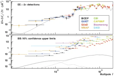
Because this polarizing mechanism is associated with the velocity component of the oscillations, the polarization power spectrum is 90◦out of phase with the temperature power spectrum. Measurements of this signal provide an independent test of the standard model, break existing degeneracies and strengthen constraints on model parameters. In 2002 the Degree Angular Scale Interferometer (DASI) made the first detection of the polarization of the CMB [74]. The EE polarization power spectrum, measured in the range 300≤l≤450, was consistent with theoretical predictions. BICEP [27] andQUAD [53] now provide the strongest measurements at degree and subdegree scales respectively (Figure 1.4).

Tensor (Gravitational Wave) Perturbations at Decoupling

effect of inflationary gravitational waves on the CMB should be strongest on angular scales larger than the horizon size at the time of decoupling (∼1◦).

Gravitational waves created tensor quadrupole moments (Y₂±2) in the frame of scatterers at the time of decoupling by alternately stretching and compressing the wavelengths of photons propagating orthogonally to each other. Thomson scattering of this quadrupole generates both E- and B-mode polarization (in equal amount). Because scalar perturbations do not produce B-modes, B-mode polarization at large angular scales on the sky constitutes a unique signature of gravitational waves generated during inflation [67].

The relative amplitude of the gravitational wave signal is quantified by the tensor-to-scalar ratior, which is given by [83]

rl=

Cl(grav)

Cl(density)

, (1.23)

where theCl(grav)’s correspond to the gravitational wave polarization signal and theCl(density)’s

correspond to the CMB polarization generated by the dominant mechanism. The depen-dence ofrlonlis expected to be fairly weak, and a single valueris frequently defined using the ratio at the quadrupole (l= 2).

The tensor-to-scalar ratio r and the scalar spectral index ns are directly related to parameters that describe the inflationary scalar potential [72]. A measurement of rwould therefore not only confirm inflation theory, but would act to distinguish between different inflationary models and to probe the physics of the inflationary epoch [11].

As of this writing, the B-mode signal has not been detected. Currently, Keisler et al. [71] sets the best published constraint onr(r <0.17 at 95% confidence). This comes from the combination of SPT andWMAP data with distance measurements from baryon acoustic oscillations and current constraints on the Hubble constant. This constraint comes mostly from measurements of the tensor contribution to CMB temperature anisotropies at large scales. BICEP places the strongest published constraint based on measurement of CMB polarization (Figure 1.4). They findr <0.73 at 95% confidence [27].

detected with the next generation of CMB polarization experiments (r >0.01, equivalent to 10s or 100s of nanoKelvin rms) [20].

Rescattering at Reionization

After recombination, hydrogen in the universe was largely neutral and thus transparent to radiation. Stars had not yet formed. For hundreds of millions of years radiation was nei-ther emitted nor scattered at significant levels except at characteristic hydrogen absorption energies. This period is known as the cosmic “Dark Ages.”

An expanding universe full of neutral hydrogen presents an opaque barrier to ultraviolet photons emitted with energies above 10.2 eV, the rest frame Lyman-αenergy. Over time photons that start out with energies above 10.2 eV are redshifted down and then promptly absorbed. Even a very small residual of neutral hydrogen presents a formidable absorption barrier. The absence of the resulting Gunn-Peterson absorption trough in quasar spectra at redshiftz < 6 is strong evidence that intergalactic hydrogen went through a period of reionization and is now almost entirely ionized. In 2001, two separate detections were made

ofz > 6 quasars demonstrating a Gunn-Peterson trough [38, 12]. This places the tail end

of the reionization process aroundz= 6.

The Dark Ages were ended by the formation of luminous compact objects capable of emitting enough energy to ionize hydrogen on large scales. It is still uncertain what kinds of objects were the dominant source of this power. Leading theories favor Population III stars (never observed) as the primary catalysts for reionization [6, 8]. The details of this important transitional epoch are still poorly understood.

ionization. Planck’s deep full sky polarization measurements will greatly improve our understanding of this important epoch.

Gravitational Lensing

Large concentrations of mass curve space time and act as lenses bending the paths of pho-tons. Gravitational lensing of CMB E-mode polarization distorts the polarization pattern and produces a small signal on the sky that includes B-modes as well as E-modes [125]. This is expected to be the dominant source of B-mode signal at small angular scales, peaking around 10’. Experiments that probe deeply with high resolution (like SPTpol [93]) will be best equipped to characterize the lensing B-mode signal. The power spectrum of the B-mode lensing spectrum depends on the matter power spectrum. Measurements of the lensing signal will be used to probe the matter distribution, the sum of the neutrino masses and the dark energy equation of state [36, 112].

1.7

Polarized Foregrounds

Polarized galactic foreground emission dominates over the CMB B-mode signal on average over the full sky [40, 119]. At microwave frequencies synchrotron radiation, dust emission and free-free emission (bremsstrahlung) are the relevant diffuse foregrounds [40]. Dust is dominant above around 90 GHz and synchrotron dominates at lower frequencies. Free-free emission is subdominant to dust and synchrotron at all frequencies. The Earth’s atmosphere is expected to exhibit negligible linear polarized emission from a balloon-based observing platform [57].

assumes two dust components and fits four parameters. It is used in simulations by most CMB experimental groups, includingSpider.

Electrons moving through the galaxy are accelerated in a circular motion perpendicular to the galactic magnetic field. As they spiral in a helical motion along field lines they emit synchrotron radiation [109]. The spectrum of synchrotron emission can be approximated by a power law with a negative exponent,Iν ∝ν−s. Averaging over the elliptically polar-ized emission from individual electrons, bulk synchrotron emission can be highly linearly polarized in the direction orthogonal to the magnetic field. WMAP has produced robust full sky maps of synchrotron emission on angular scales of>1◦[49, 58, 97].

-l(l+1)C

l

/ 2

π

(

μ

K

2 )

10-2 10-1 1 10 102

10-3 10-2 10-1 1 10 102

102 103

l Multipole EE:>2σ detections

BB: 95% confidence upper limits

BICEP

QUIET

QUaD

WMAP

CBI

CAPMAP Boomerang

DASI

Chapter 2

The S

PIDER

Balloon-Borne CMB

Polarization Experiment

TheSpiderCMB polarization experiment [32, 42, 45] is specifically designed to search for the CMB inflationary gravitational wave B-mode signal. Because this signal is expected to be faint in comparison with polarized galactic foregrounds, Spider will observe the microwave sky in three frequency bands to discriminate between the CMB and galactic foregrounds based on their distinct spectral signatures (§2.2). Spiderwill target a field not heavily contaminated by galactic dust, mapping a large region in the southern sky (§2.3). Observing 9.5% of the full sky with∼1◦beams maximizesSpider’s sensitivity to angular scales between 1◦and 10◦. These moderate angular scales correspond to the multipoles 10<

l <100 where the inflationary B-mode signal peaks. To minimize response to atmospheric

fluctuations and reduce photon noise and loading,Spiderwill observe from a long duration balloon in the relatively stable low background environment above the troposphere (§2.4).

To mitigate risk the designs of Spider’s optical, cryogenic, magnetic shielding, and attitude systems (§2.4–§2.6) favor simplicity and the use of proven technologies where possible. The attitude control system is based on the configuration flown successfully on

Institution Institution Lead Principal Responsibilities

Princeton William Jones* Cryogenics and system integration Caltech and JPL James Bock Receiver fabrication and testing U. Toronto C. Barth Netterfield Gondola and flight systems Case Western John Ruhl Stepped cryogenic half-wave plates

NIST Kent Irwin SQUID multiplexing readout system

U. British Columbia Mark Halpern Warm readout electronics Cambridge Carrie MacTavish Simulations

Cardiff Peter Ade Filters

Table 2.1: Spider collaborating institutions. William (Bill) Jones is the Principal Investi-gator. Andrew Lange was the proposing Principal Investigator, and led the team until his death in 2010.

2.1

Collaboration

TheSpider collaboration is composed of expert institutions in each of the major compo-nent subsystems (Table 2.1). Many of the senior members were leading participants in the very successfulBOOMERanGcollaboration [89, 90, 31]. Locally, Caltech is responsible for receiver design, detector characterization, optics, and magnetic shielding. NASA JPL fabri-cates the antenna-coupled TES detectors and integrates them into focal planes. My primary responsibilities have been in detector development with Jamie Bock and the JPL detector fabrication team, and in the characterization ofSpider’s overall receiver performance with other Caltech collaborators.

2.2

Frequency Coverage

On large angular scales the B-mode CMB polarization signal is faint in comparison with the polarized galactic foregrounds due to synchrotron and thermal dust emission [40, 119]. Confusion with polarized astronomical foregrounds sets the ultimate limit on measurements of CMB polarization on large scales. Accurate modeling and mapping of foreground signals is therefore crucial to isolating the CMB polarization signal. Because synchrotron emission, dust emission, and the CMB each have unique spectral signatures, mapping the microwave sky at multiple frequencies enables foreground mapping and subtraction.

Focal Plane

Flight Frequency Distribution

Spider 1, December 2012 3×93 GHz; 3×148 GHz Spider 2, December 2014 2×93 GHz; 2 ×148 GHz; 2×280 GHz

Table 2.2: Planned frequency distribution of focal plane units and timeline for Spider’s first and second flights. Spider is a modular instrument with bays for six independent monochromatic telescopes.

Planck LFIwill map synchrotron emission with increasing sensitivity in coming years. Polarized thermal dust emission becomes dominant above around 90 GHz and increases with frequency. However, its properties are not well constrained by the published literature, especially off of the galactic plane. Planck HFI has been observing for more than a year with bands at 100, 143, 217, 353, 545, and 857 GHz [77]. Planck’s recent release of full sky images of the galaxy in all six HFI bands emphasizes the ability of this data set to characterize the spectral energy density of the dust emission intensity [101]. In 2012

Planck will release calibrated time-ordered data, full sky maps at each frequency, full sky component maps (CMB and galactic foreground emission), and a final compact source catalog.

Spider will map the off-galaxy southern sky with bands centered at 93, 148, and ∼280 GHz, each with a ∼25% bandwidth. The planned frequency distribution of focal plane units for each flight is tabulated in Table 2.2. In its first flight,Spiderwill map the sky in the prime 93 and 148 GHz bands where the CMB signal is the strongest. Based on our foreground model, we expect to begin to detect polarized dust emission in the 148 GHz band in the first flight. The∼280 GHz band (not yet designed or fabricated) will be added in the second flight to provide greater leverage for discriminating, mapping and subtracting polarized interstellar dust emission. This band will also complement thePlanckdata set by filling in the gap in its frequency coverage.

í

í

$WPRVSKHULF(PLVVLRQDQG*DODFWLF&2/LQHV

>*+]@

(PLVVLRQ,QWHQVLW\>S:*+]@

&2

-í _-í&2

2

2

+2

+2

&2 -í

*+] *+] *+]

Figure 2.1: Spider will observe in bands centered at 93, 148, and∼280 GHz to minimize response to atmospheric emission lines and to galactic CO emission lines.

Red: The power density [pW/GHz] of atmospheric emission based on a model for mid-latitude emission at 30 km altitude [98]. Black dashed: The frequencies associated with rotational transitions of galactic12_C16_{O [30]. CO emission intensity should vary significantly}

−20 0 20 40 60 80 100

−60

−40

−20 0

−20 0 20 40 60 80 100

−60

−40

−20 0

Figure 2.2: Left: Polarized dust amplitude at 150 GHz, according to the model in [95] (0–5μKCMB, linear scale). TheSpiderobserving region (outlined in white) covers most of the southern sky not heavily contaminated by dust. The southern Galactic pole (black +) is overplotted, along with the 10- and 20-degree galactic latitude lines (dashed). Also shown are the BICEP and BOOMERanG fields (gray outlines), and the region of minimum foreground contamination in the Spider field (purple outline). Right: Distribution of integration time (linear scale), averaged over all detectors in a single 148 GHz focal plane for the observing strategy discussed in §2.4. This observing profile covers 10% of the sky, of which 85% is observed with near-isotropic coverage in crossing angles. Figure from [45].

2.3

Sky Coverage

Spider will map most of the southern sky not heavily contaminated by galactic dust, for a total of 10% of the full sky (Figure 2.2). With subdegree beam sizes (30’ at 148 GHz),

Spideris most sensitive to correlations on angular scales between 1◦and 10◦. These scales correspond to spherical harmonics with multipole moments 10< l <100.

Spider’s sky coverage is more expansive than that of experiments such as SPTpol, which will target larger multipoles with its smaller beams and provide strong sensitivity to the gravitational lensing signal. Planck will map the full sky and therefore achieve sensitivity to the lowest monopoles (2 < l < 10). Planck is in a unique position to measure the reionization peak in the polarization power spectra atl < 10. In fact, all of

Planck’s sensitivity to the inflationary B-mode signal is in the reionization peak at very large angular scales. TheSpider and Planckdata sets will provide very complementary probes of the inflationary gravitational wave signal.

2.4

Ballooning

Out-side of the scientific community microwaves are best known for their use in heating food because the dielectric H2O, common in foods, interacts efficiently with microwaves. Water

vapor in the Earth’s atmosphere emits a significant amount of energy in a continuum across the microwave bands of interest to CMB science. This atmospheric emission contributes both photon noise and loading. Because water vapor density is inhomogenous and tem-porally variable, it is particularly difficult to effectively subtract from measurements made over large angular scales. Atmospheric noise is also especially onerous in higher frequency bands (above 150 GHz), as the CMB intensity is dropping off with frequency while the atmospheric noise is increasing (Figure 2.1).

Most (∼99%) of the water vapor in the Earth’s atmosphere is in the troposphere, the lowest portion of the Earth’s atmosphere. Spider will observe from above the troposphere at an altitude of∼32 km on long duration balloon flights provided by NASA’s Columbia Scientific Balloon Facility (CSBF). The balloon platform provides a relatively stable low background environment for observing. Each balloon flight will launch from McMurdo, Antarctica and will circle the continent for about 20 days guided by the polar vortex winds. At the completion of the flight,Spiderwill separate from the balloon and free fall toward the Earth. A parachute will open to slow the descent of the payload, which will then be recovered from the Antarctic ice fields and recommissioned for the next flight.

Ballooning puts a number of constraints on any experiment. These include power con-straints, lack of physical access to the instrument during operation, limited in-flight commu-nication bandwidth, and mass constraints. The specific technical requirements of balloon-ing and satellite missions are similar, makballoon-ingSpideris a particularly good pathfinder for the proposed Experimental Probe of Inflationary Cosmology (EPIC) orbital mission [16].

Spider will pioneer multiple technologies for the EPIC satellite, just as its predecessor BOOMERanGpioneered technologies forPlanck.

weight and, where possible, materials have been chosen accordingly.

The University of Toronto is responsible for theSpidergondola, which is the mechanical structure that couples theSpiderinstrument to the balloon and scans the telescope. Tra-ditionally gondolas for balloon-borne experiments are constructed from welded aluminum. For weight reduction, theSpidergondola frame is constructed from carbon fiber reinforced polymer tubes with aluminum joints. Both finite element analysis (FEA) and physical pull tests on individual components have demonstrated compliance with requirements for strength and stiffness. Stiffness requirements are driven by the need to maintain pointing accuracy as the system center of mass shifts due to cryogen boil off and ballast drops. The system is designed with adequate strength to accommodate a parachute deployment accel-eration of up to 10 g. An impact attenuation system supplied by CSBF and attached to the bottom of the gondola controls the large forces on landing. The base of this system is large to reduce the probability of rolling. To protect the cryostat in the event of a rollover, the front of the gondola frame extends forward to a rollover bar.

Spiderwill utilize a reaction wheel to perform back and forth continuous antisun scans in azimuth with steps in elevation. An active pivot between the balloon flight train and the gondola compensates for balloon rotation. The motorized reaction wheel can spin the gondola with a 0.8◦/s2 _{maximum acceleration and 6.0}◦_{/s maximum speed. The elevation}

drive is driven by two linear actuators and allows adjustment from 22◦to 52◦. The baseline scan strategy calls for elevation steps of 1◦every hour, from 28◦to 40◦and then back again. The instrument completes an entire scan cycle in one day. The amplitude and center of each azimuth scan is selected at each elevation to remain in the low foreground off-galaxy southern sky and to avoid approaching within 90◦ of the sun.

expect an rms uncertainty of 1’ inSpiderpointing reconstruction. Regular observations of bright compact sources during flight will be used to monitor beam centroid offsets.

2.5

Cryogenics

The team at Princeton University is responsible for the design and characterization of the

Spider flight cryostat, which was custom built by Redstone Aerospace1. The thermal architecture of the cryostat is shown in Figure 2.4 and described in detail in Gudmundsson et al. [52]. With a 1,284 L main helium tank maintained at∼1 atm, the unit is designed to provide at least a 25-day hold time. Helium gas boil off from the main tank is coupled through heat exchangers to inner and outer vapor-cooled shields (VCS1 and VCS2) that thermally shield the 4 K stage. The enthalpy of the gas provides sufficient cooling to these stages to obviate the use of liquid nitrogen, simplifying design and reducing mass. The long narrow winding vent tube is susceptible to nitrogen ice plugs, so care is taken to maintain a positive outflow of gas during cryogen fills and operation. The helium bath and vapor-cooled shields are encased in a cylindrical vacuum vessel 2.05 m tall and 2.43 m in diameter. The dry weight of the cryostat (no LHe or telescope inserts) is about 850 kg.

Inside the inner radiation shield (VCS1) a small 16 L superfluid helium tank is capillary fed by the main helium tank. This tank will be vacuum pumped to a few hundred pascal prior to launch and then capped off. At float a valve will open to vent the tank to ambient atmospheric pressure (∼100 pascal), which will maintain the helium in its superfluid state at a temperature of about 1.6 K. This cooling point is used to cycle the 3He adsorption refrigerators that cool each focal plane.

The cryostat was designed to sustain nonparasitic heat loads of 12 mW, 550 mW, 4 W, and 9 W to the superfluid tank, main tank, VCS1 and VCS2, respectively. As of this writing, the cryostat has been built and is undergoing testing at Princeton. The cool down process takes about a week from 300 K to 300 mK and the cryostat currently achieves a hold time of about 20 days under flightlike loading.

The sub-Kelvin focal plane architecture is described in detail in Runyan et al. [107]. An assembled focal plane assembly is pictured in Figure 2.5. Spider’s focal plane architecture (the “RevX” design) differs from the (“RevE”) architecture employed byKeck(our sister

Figure 2.5: Left: An assembled focal plane unit with the A4K outer shield (“spittoon”) removed. The spittoon is mechanically supported by black carbon fiber rods from the aluminum 4 K plate and cooled by copper straps bolted to the 1.6 K ring. The sub-Kelvin stage is mechanically supported off of this 1.6 K ring, and cooled by the3_{He fridge. The gold}

plated copper detector plate, with a Cernox thermometer and heater, is coupled to this cold stage by (diagonal) stainless steel struts which act as a passive thermal filter. The square niobium box which encases the SQUID multiplexing system is visible just behind these struts. Right: 3He adsorption refrigerator mounted on a gold-plated aluminum plate (4 K). A copper thermal bus bar feeds through the plate (right side of image) to couple the fridge condensation point to the superfluid helium bath (1.6 K).

experiment on the ground) due to more stringent magnetic shielding requirements (discussed in§2.8). Marc Runyan performed much of the focal plane redesign, which has substantially reduced magnetic pickup in the SQUID system (see§4.9).

A gold-plated aluminum cold plate at the base of each telescope insert mounts to the main liquid helium tank. The optics truss structure and a simple closed-cycle 3He ad-sorption refrigerator are mounted on this plate. A 1.6 K gold-plated copper bar from the superfluid helium tank is fed through a hole in the base plate to provide cooling to the fridge condensation point as well as to a magnetic shield and to the blackened cold sleeve which lines the optics tube. The 10 stp-liter3He fridges (one pictured in Figure 2.5) are produced by Simon Chase Research. They can provide a steady base temperature of around 300 mK to the detector plate with a hold time of three days. In flight they will be recycled every 72 hr.

condense in to the still for 30 min. We then turn off the pump heater and apply 0.7 mW to the heat switch to cool the pump.

The fridge cools the focal plane through eight stainless steel blocks that are gold plated on either end to minimize thermal impedance. We have measured a total thermal impedance from fridge to focal plane of 2.3 mK/W. Stainless steel has a large heat capacity, so the blocks act to filter out any high-frequency thermal fluctuations on the fridge side of the thermal link. The 3 dB point of the thermal transfer function has been measured at 2 mHz. Four detector tiles are secured against the square detector plate with beryllium copper clips and are held in alignment by pins and slots. Over a hundred gold wire bonds per tile make a thermal connection between the gold-plated copper plate and large gold bond pads near the edge of the detector tile (Figure 3.3). Becky Tucker has measured an overall plate-to-tile thermal conductance of 245μW/K at 300 mK (limited by Kapitza resistance). An NTD Ge thermistor is mounted on each tile for temperature monitoring.

A niobium back short is positioned a quarter-wave distance behind the detectors to define a boundary condition that forces constructive interference at the antenna. All stages of the SQUID multiplexing system are behind the back short encased in several layers of magnetic shielding. Superconducting electrical connections between the TES detector tiles and the SQUID system are achieved through the use of flexible aluminum circuits and aluminum wire bonds.

2.6

Optics

Spideris an array of six individual monochromatic telescopes encased in a single cryostat housing (see Figure 2.6). Modularity simplifies half-wave plate design and antireflection coating of optical components because each individual telescope tube operates in a single frequency band. Pairs of telescopes observing in each band are oriented such that their polarization sensitivity differs by 45◦. This enables simultaneous measurement of the Stokes parametersQand U.

Figure 2.6: The Spider flight cryostat can accommodate up to seven modular telescope inserts. However, we only plan to instrument the outer six insert bays. The inner bay may be used for thermal busses and a carbon getter to improve the quality of the vacuum. Telescope inserts (Figure 2.7) slide in to the bottom of the cryostat and bolt at the base, as shown in the image at right.

.&ROG 3ODWH

+H6RUSWLRQ

)ULGJH

$X[3RVW . )RFDO3ODQH

P.

/HDG6KLHOG . $. 6SLWWRRQ

.

(\HSLHFH /HQV.

2EMHFWLYH /HQV. &RROHG%ODFN

2SWLFV6OHHYH .

0HWDO PHVK)LOWHU

.

.)LOWHUV &RSSHUFODG

*:UDS.

2SWLFDO6WRS .

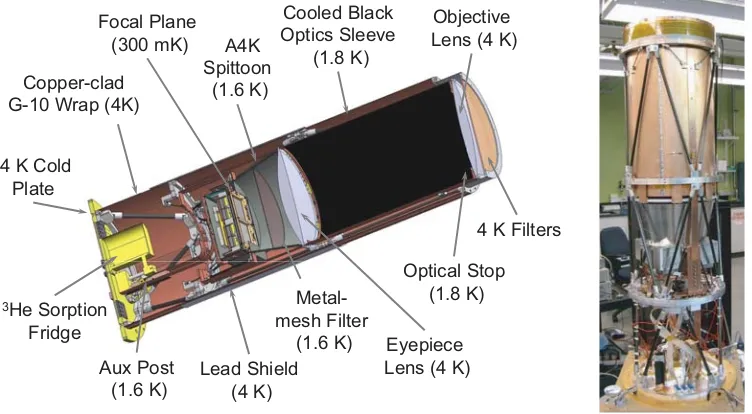
Figure 2.7: Left: Cross-sectional drawing of a telescope insert. Drawing credit: M. Runyan.

preflight characterization in the far field of the optics becauseD2/λ≈30 m.

A cross section of the optics tube is shown in Figure 2.7, and Spider’s optics are described in Runyan et al. [107]. A blackened sleeve lines the inside of the telescope tube between the eyepiece and objective lenses. The blackened Lyot stop caps the top of this sleeve just below the objective lens, preventing beam spillover on to warmer surfaces skyward of the objective. The antenna beam is approximately a sinc function, and the telescope aperture nearly coincides with the null between the main beam and the four primary side lobes. Primary and secondary side lobes are all terminated inside the telescope on the blackened stop and sleeve. Because 25% of the antenna beam power is in these side lobes, we achieve a substantial reduction in in-band loading (§4.5) by cooling the sleeve and stop to 1.8 K using the superfluid helium tank. The lenses and wave plate are cooled to 4 K using the main helium tank. Decreasing loading reduces photon noise in the detectors, allowing

Spider to better take advantage of the favorably low atmospheric loading conditions at float.

Spider’s optical design is based on theBICEPdesign [124] and its lenses are identical to those of BICEP2. The lens optimization process is discussed in Aikin et al. [2]. The plate scale is 0.98◦/cm at the focal plane and the corner-to-corner field of view of each insert is 20◦. High-density polyethylene slabs used for Spider’s lenses are annealed to relieve stress before they are rough cut, before final machining, and again as part of the antireflection coating process. CMM surface metrology confirms that the correct figure has been achieved. During cooling to 4 K the HDPE lenses contract by 2% while the aluminum rings that support them contract by only 0.4%. For this reason, the lenses are held in place by equally spaced 1/32” thick copper flexures which absorb the differential contraction, keep the lenses centered, and provide a cooling path to the 4 K helium bath.

The rest of Spider’s filter stack packs tightly in to the space between the objective lens and the vacuum closeout window. A 3/32” thick nylon filter and a hot-pressed filter (10 cm−1 cutoff for the 148 GHz band) are mounted on the telescope insert structure just skyward of the objective lens at 4 K. The half-wave plate (§2.7) is next in the optical train, secured to the cryostat itself at 4 K. A hot-pressed filter (12 cm−1 _{cutoff for the 148 GHz}

band) and three IR shaders intercept radiation at the first vapor-cooled shield (VCS1). The VCS1 stage equilibrates just above 10 K in the Spider test cryostat and around 30 K in theSpiderflight cryostat. Four IR shaders mount to the∼90 K VCS2 stage.

The vacuum enclosure is sealed by a thin window above each telescope insert. The current plan is to use 0.001” thick teflon for these windows, but this may be changed as it has been suggested that teflon can introduce undesirable beam effects. The thin windows are protected from atmospheric pressure while on the ground by much thicker windows, which retract when the instrument reaches float altitude.

Reflections can introduce ghost beams. A reflective niobium back short is located a quarter-wave distance behind the detector plate to set up constructive interference in the plane of the antennas. The lenses, nylon filter, hot-pressed filters, half-wave plate, and silicon detector wafers are all coated with quarter-wave antireflection coatings ([51],§4.4). NSG-N quartz antireflection tiles are sandwiched between the sky side of the silicon detector tiles and the detector plate. For the lenses and nylon filters we use Porex2 porous Mupor membranes because they are pliable and available with indices and thicknesses well matched to our lenses and filters. We select PM23DR for the HDPE lenses and PM23JR for the nylon filters. Adhering the Porex coatings is most difficult on the curved lens surfaces. A silicon vacuum bag presses the coatings firmly and evenly against the lens (or filter) as it rests on a matching concave (or flat) aluminum plate. A thin, low-density polyethelene (LDPE) sheet is then melted (10 hr at 124◦C) at the interface between them. This lamination process has been successfully demonstrated, with wrinkle-free coatings showing no signs of delamination after10 thermal cycles. The nylon and teflon surfaces are abraded with Scotchbrite and then thoroughly cleaned prior to bonding. When coating lenses, the LDPE film must be prestretched to match the curvature of the lens to avoid wrinkling. Porex materials easily pick up static charge, dust, and oils, and should be handled using gloves.

Figure 2.8: Left: A sapphire half-wave plate mounted in the optical receiver test bed at Caltech. Right: The rotor is coupled to a stepper motor by a worm gear.

2.7

Half-Wave Plates

To modulate polarization sensitivity in flight,Spiderutilizes cold (4 K) stepped sapphire half-wave plate (HWP) assemblies developed at Case Western Reserve University and de-scribed in Bryan et al. [25]. Each telescope insert employs a single HWP located just skyward of the objective lens (see Figure 2.8). In flight the plates will all be rotated by 22.5◦ daily. This rotates the polarization sensitivity of the focal planes and allows each pixel to measure both Stokes parameters Q and U. Following each HWP rotation, the instrument will scan compact sources for about 30 minutes to check pointing offsets and beam profiles. The HWP rotates the polarization sensitivity of the telescope without rotat-ing the beam, mitigatrotat-ing systematic effects due t